Computer-network Solutions for Pervasive Computing

(1)

Department of Information Engineering, University of Pisa, Italy Ph.D. Thesis - XIX Cycle

Computer-network Solutions

for Pervasive Computing

Ph.D. Candidate

Luciana Pelusi

Advisors

Prof. Giuseppe Anastasi

Dott. Marco Conti

(2)

(3)

(4)

(5)

3.3.1. Encoding Process . . . 173 3.3.2. Decoding Process . . . 173 3.3.3. Applications . . . 175 3.4. Raptor Codes . . . 176 3.4.1. Encoding Process . . . 176 3.4.2. Decoding Process . . . 177 3.4.3. Applications . . . 178 4. Network Coding . . . 179 4.1. Encoding Process . . . 182 4.1.1. Recursive Encoding . . . 185

4.1.2. How to choose encoding vectors? . . . 188

4.1.3. Generations . . . 189

4.2. Decoding Process . . . 190

c

(8)

4.3. Applications . . . 192

5. Conclusions and Open Issues . . . 194

VI. Reliable Data Collection in Sparse Sensor Networks 197 1. Introduction . . . 197

2. Unreliability issues in Sparse Wireless Sensor Networks . . . 199

2.1. One-hop reliability . . . 201

2.2. End-to-end reliability . . . 203

2.3. Encoding-based Solutions . . . 204

3. Preliminary Results from a Small-scale Testbed . . . 208

3.1. Testbed Description . . . 208

3.2. Experimental Results . . . 210

(9)

List of Figures

II.1. Streaming architecture for a wireless scenario. . . 17 II.2. Streaming model under real-time constraints: graphical model. . . 20 II.3. Available bandwidth estimates for different client buffer size and

WNIC data rate. . . 26 II.4. Available bandwidth estimates for different client buffer size and

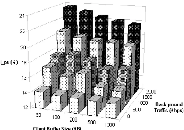
background traffic. . . 28 II.5. I_ps experienced by a streaming flow competing with CBR

back-ground traffic. Min burstness: 1 packet per single burst. . . 30 II.6. Variations in the client buffer level during the streaming session.

The client buffer size is 1000 KB. No background traffic is present. . 32 II.7. Variations in the client buffer level during the streaming session.

The client buffer size is 1000 KB. Maximal background traffic is present. . . 32 II.8. I_ps experienced by a streaming flow competing with a bursty CBR

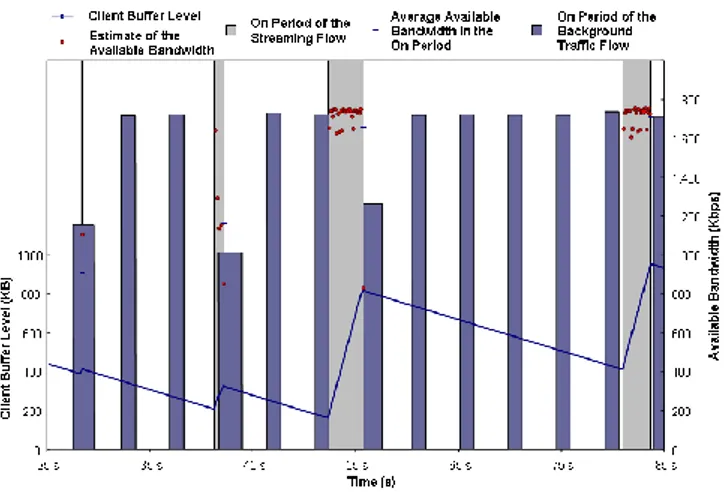
traffic. Max burstness: 200 packets per single burst. . . 34 II.9. Variations in the client buffer level during the streaming session.

The client buffer size is 1000 KB. The background traffic is 500 Kbps with 200 packets sent per single burst. . . 34 II.10.Variations in the client buffer level during the streaming session

from 25 s to 85 s. The client buffer size is 1000 KB. The background traffic is 500 Kbps with 200 packets sent per single burst. . . 35 II.11.Two competing streaming flows with no background traffic: I_ps

experienced when combining different client buffer sizes for the two flows. . . 37

(10)

II.12.I_ps experienced in two competing streaming flows when adding

background traffic of different types. . . 38

III.1. Reference Architecture . . . 44

III.2. Experiments Area . . . 49

III.3. Experiments Scenario . . . 50

III.4. Routing Network Topology . . . 57

III.5. OLSR overhead . . . 59

III.6. AODV overhead . . . 60

III.7. OLSR overhead in case of disconnection event . . . 61

III.8. AODV overhead in case of disconnection event . . . 61

III.9. Network Topology for FreePastry Experiments . . . 62

III.10.Traffic Load on each node running Pastry on top of OLSR . . . 64

III.11.Traffic Load on each node running Pastry on top of AODV . . . 64

III.12.Node F traffic on an OLSR network . . . 65

III.13.Node F traffic on an AODV network . . . 66

III.14.Node A traffic profile (AODV case) . . . 67

IV.1. Example of network-coding efficiency. . . 110

V.1. Encoding, transmitting and decoding processes for the data origi-nated at a source. . . 152

V.2. A graphical representation of the encoding and decoding processes of an (n, k)-code. . . 157

V.3. The encoding/decoding process in matrix form, for systematic code (the top k rows of G constitute the identity matrix Ik). y0 _{and G}0 correspond to the green areas of the vector and matrix on the right. 163 V.4. The arrangement of data and the transmission order at the server. . 165

V.5. Waiting for the last blocks to fill. . . 166

V.6. (a) A bipartite graph defines a mapping from message bits to check bits. (b) Bits x1, x2, and c are used to solve for x3. . . 167

V.7. The code levels. . . 169

(11)

List of Figures vii V.9. Raptor Codes: the input symbols are appended by redundant

sym-bols (dark squares) in the case of a systematic pre-code. An ap-propriate LT-code is used to generate output symbols from the pre-coded input symbols. . . 177 V.10.Relay nodes perform encoding over n ingress data packets and

pro-duce m data packets to send out. The number of encoded packets is greater than the number of incoming data packets. . . 180 V.11.A one-source two-sink network with coding: link capacities (left)

and network coding scheme (right). . . 180 V.12.All the packets have the same length of L bits. Shorter packets are

0-padded. . . 183 VI.1. Reed-Solomon Code and Network Coding: differences and

similar-ities. . . 206 VI.2. Mica2 motes. . . 209 VI.3. MIB500CA Programming Board. . . 210

c

(12)

(13)

List of Tables

II.1. Symbols used in the Streaming Model. . . 20 II.2. I_ps vs. Client Buffer Size. Worst Case: 2 Mbps Data Rate, 2 Mbps

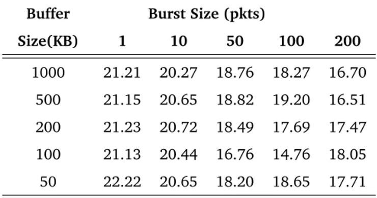
Background Traffic. . . 31 II.3. I_ps vs. Burst Sizes in the Background Traffic. 1 Mbps Background

Traffic, 2 Mbps Data Rate . . . 33 VI.1. Mica2Motes features. . . 209

(14)

(15)

I. Introduction

The last decades have witnessed a revolutionary change in the computing model with the advent of mobile wireless communications. In the nineties, mobile com-puting devices (e.g., laptops, personal digital assistants and other generic hand-held digital devices like cellular phones), have finally met consensus of users and experienced widespread diffusion. Users have discovered the possibility to access all the information they require whenever and wherever needed and have inter-estingly changed their habits in using computers. While before nineties the use of computing devices was only concerned with job and study, and devices were intended to be powerful desktops located in offices, at home or even in Internet cafes were Internet access were provided, in the so-called mobile computing age, people have experienced, and enjoyed, new ways to take advantage from digital devices and have thus started to utilize different electronic platforms at the same time. Mobile access to the Internet has been one of the first incentives to the use of portable computing devices. Mobile users have started to utilize their cellular phones to check e-mails and browse the Internet, and travelers with portable com-puters have begun surfing the Internet from airports, railway stations, and other public locations.

From then on, ever more powerful mobile devices have come to the market thank to the rapid progresses in both hardware and software. These days portable com-puters do not only replicate but almost substitute desktop comcom-puters. But the most interesting evolution consists in the ongoing proliferation of even more smaller devices pervading the environment, from PDAs to wearable computers, and to de-vices for sensing and remote control. This current age has therefore been named Ubiquitous Computing age [Wei91], or Pervasive Computing age [Sat02]. These definitions refer to an environment which is saturated with computing and

(16)

com-munication capabilities aimed to help users in their everyday life but without re-quiring any major change in their behavior. Virtually everything in this environ-ment (from key chains to computers, and PDA’s) is connected into a network, and can originate and respond to appropriate communications. Similar environments are not actually deployed yet, but a physical world with pervasive, sensor-rich, network-interconnected devices embedded in the environment is envisaged as the next generation computing challenge [ECPS02].

The nature of ubiquitous devices makes wireless networks the easiest solution for interconnection. Furthermore, mobility is a fundamental part of everyday life. Hence, wireless and mobile communications are a fundamental building block for smart pervasive computing environments. Currently, wireless connec-tivity is generally provided by wireless LANs (conforming, for example to the IEEE 802.11WLAN standard), or somewhat smaller and less expensive Bluetooth de-vices. However, in a pervasive computing environment, the infrastructure-based wireless communication model is often not adequate because it takes time to set up the network infrastructure and the costs associated with installing the in-frastructure can be quite high. These costs and delays may not be acceptable for dynamic environments where people and/or vehicles need to be temporar-ily interconnected in areas without a pre-existing communication infrastructure (e.g., inter-vehicular and disaster-relief networks), or where the infrastructure cost is not justified (e.g., in-building networks, specific residential communities networks, etc.). In these cases, infrastructure-less or ad hoc networks provide a more efficient solution. The simplest ad hoc network is a peer-to-peer net-work formed by a set of stations within communication range of each other that dynamically configure themselves to set up a temporary single-hop ad hoc net-work. The widespread adoption of the Bluetooth technology in computing and consumer electronic devices makes the Bluetooth piconet the most relevant solu-tion for single-hop ad hoc networks. However, a single-hop ad hoc network only interconnects devices that are within the same transmission range. This limita-tion can be overcome by exploiting the multi-hop ad hoc (MANET) technology. In a MANET, the users’ mobile devices cooperatively provide the functionalities usually provided by the network infrastructure (e.g. routers, switches, servers). Devices that are not directly connected, communicate by forwarding their traffic

(17)

CHAPTER I. INTRODUCTION 5 via a sequence of intermediate devices.

Sensor nodes are an important component of pervasive systems, and wireless ad hoc networking techniques also constitute the basis for sensor networks. However, the special constraints imposed by the unique characteristics of sensing devices, and by the application requirements, make many of the solutions designed for multi-hop wireless networks (generally) not suitable for sensor networks. For this reason, the ad hoc networking research community has recently generated an extensive literature dedicated to sensor networks.

This thesis goes through the above wireless scenarios, from the widely deployed WLANs to the emerging Opportunistic Networks. Some of the most relevant aspects of wireless pervasive systems are reviewd, starting from energy efficiency, going further to connectivity and reliability issues in transmissions.

In infrastructured wireless scenarios, like WiFi hotspots, the presence of base sta-tions, specifically Access Points (APs), guarantees high connectivity and high band-width to the nodes in their proximity. However, only limited coverage is available and this solution seems to be suitable only for temporary user needs, or for users with limited mobility. Moreover, a WLAN is to be considered an extension of the wired Internet, in fact, scenarios with mobile wireless devices accessing the Inter-net via APs are generally referred to as wireless InterInter-net. These environments pro-vide the same identical kinds of services as the wired Internet. Hence, their major requirement is to guarantee the same service quality as the wired Internet. This implies masquerading the last wireless connection between the AP and the mobile device. A key issue in wireless Internet is energy efficiency since portable devices are battery-fed and have therefore limited energy budget. Though technological progress has been producing in the last few years ever more powerful batteries, the increased usage of portable devices has also led to higher energy requirements. Hence, software solutions are currently being deployed to avoid energy wastage at the wireless devices during their common activity. When integrating energy saving support into the classical Internet applications, service provisioning in the wireless Internet is possible for a longer time. The most efficient energy saving solutions are those which save energy during networking activities since they have been demonstrated to be the most energy-hungry activities. Chapter II focuses on

c

(18)

the diffusion of multimedia streaming services in smart environments and specifi-cally investigates scenarios where mobile users who have a Wi-Fi access to the In-ternet receive audio files from remote streaming servers [ACG+_06a_{] [}_ACG+_05a_].

When dealing with these applications, particular attention must be taken to qual-ity of service(QoS) requirements, and the solutions for optimization of resource consumption must not degrade the QoS perceived by the user. Energy saving is addressed by including periodic transmission interruptions in the schedule of au-dio frames at the server, such that the network interface card at the receiver can be set to a low-power consuming state. Experimentation on a software prototype shows that the solution proposed makes possible energy savings ranging from 76%to 91% (depending on the data rate and the background traffic) of the total consumption due to the network interface. Good user level QoS is also preserved. Infrastructure-less ad hoc networks have their strength in the absence of infras-tructure which means that they can be set up very fast and with minimum effort and low cost (only that of the wireless network interface card). Much work on wireless ad hoc networks has been conducted so far, mostly through simulation modeling and theoretical analyses. Instead, relatively few experiences with real ad hoc networks have been performed, and the results from these experiences do not always validate simulative conclusions. So, analytical and simulative re-sults have to be complemented by real experiences (e.g., measurements on real prototypes) which provide both a direct evaluation of networks and, at the same time, precious information to realistically model these systems and avoid unreal-istic simulation settings. Chapter III presents and discusses some lessons learned from an experimental work on a wireless ad hoc testbed [BCDP04]. Specifically, results are presented for a fully functioning prototype implementing a p2p mid-dleware (FreePastry) on top of a multihop ad hoc network based on IEEE 802.11b technology . Recently, for this technology, [GLNT] has pointed out the existence of an ad hoc horizon (2-3 hops and 10-20 nodes) after which the benefit of multi-hop ad hoc networking vanishes. All the experiments performed fall inside this ad hoc horizon. The aim of the experimentation has been to identify solutions for this realistic setting and to quantify the Quality of Service (QoS) that the system is able to provide to the users. The measurements performed have pointed out that also in this limited setting, several problems still exist to construct efficient

(19)

CHAPTER I. INTRODUCTION 7 multi-hop ad hoc networks. Cross-layering seems to be an effective approach to fix some of the problems identified in this analysis.

The feasibility of an ad hoc network is related to the attitude of nodes to stay in group such that they can communicate directly with each other (over single-hop connections) or through intermediate nodes over multi-hop connections. In both cases, communications rely on a certain knowledge of the network topology, at least of the path to the destination node. So, when a node has to send data to a destination node, it collects information about the reachability of that node. Then it sends out the data only if the destination node is actually reachable, along a pre-determined path, otherwise it discards the data. This is exactly what hap-pens in the wired Internet where a message is either forwarded immediately or considered undeliverable. Actually, in wireless environments with high mobility, the network topology is continuously varying and it is possible that messages that cannot be delivered at a certain time can be delivered a few time later instead. Novel communication paradigms currently under study do not rely on the pres-ence of a complete path towards a destination node but rather exploit delivery probabilities towards that destination node, referring to the possibility that a path to that destination will appear sooner or later. Obviously, this new communication paradigms do not suit all kinds of applications, especially real-time applications. Applications that are relatively independent of the time and can tolerate even long transmission delays are rather concerned. Chapter IV focuses on this new, emerging research area of wireless networking, known as Opportunistic Network-ing. The very characteristic of opportunistic networks is their intermittent con-nectivity, meaning that there is no assurance to the existence of a complete path between pairs of nodes wishing to communicate. Therefore, communications typ-ically happen by exploiting pair-wise contacts between nodes. A node wishing to send/forward a message looks for a next-hop. If a next-hop exists then the node forwards the message to it, otherwise it keeps the message until a new contact opportunity arises. A message gradually approaches the destination by follow-ing the motion of the nodes it is carried by and by passfollow-ing node-by-node durfollow-ing pair-wise contacts. Eventually, it reaches the destination. Contact opportunities among nodes may be scheduled over time or completely accidental. They depend on the particular network scenario and the mobility of nodes. The very novelty of

c

(20)

opportunistic networks consists in the fact that while infrastructured WLANs and infrastructure-less MANETs work despite mobility of nodes and can tolerate it up to a certain degree, opportunistic ad hoc networks actually rely on node mobility because full connectivity is not assured in any way and the probability of suc-cessful message delivery is as much higher as the nodes move and meet up with each other. This communication paradigm is particularly suitable to environments with a high number of heterogeneous devices. Opportunistic network scenarios are very challenging due to the scarceness of resources and are often referred to as extreme networks. Chapter IV overviews the theoretical foundations of op-portunistic ad hoc networks and also describes some recent experimental studies and projects in the area. Finally, it reviews the state-of-the-art of the routing and forwarding strategies used in opportunistic environnments [PPC06b] [PPC06a]. Data forwarding is surely one of the most compelling issues in opportunistic sce-narios and it concerns, in a certain sense, with guessing the best direction(s) to-wards the destination node. However, this is only part of the problem, since we can more generally talk about reliability issues in opportunistic environments and classify them into two different levels: one-hop and end-to-end reliability. One-hop reliability concerns with transmissions that occur during a contact between nodes in the communication range of each other, whereas end-to-end reliabil-ity concerns with efficacy of the data forwarding strategy applied. One-hop re-liability is affected by the duration of contact times occurring between pairs of nodes. In fact, depending on the trajectories followed by nodes and on their speed, contact times between nodes can be shorter or longer, but are generally unpredictable. The duration of contact times limits the total amount of data that can be transferred between the communicating nodes and thus the overall throughput that can be achieved. Moreover, to make things worse, it should be noted that contact times are not well-delimited. Rather, their starting point and ending point can be inferred from the loss pattern which is experienced during transmissions [ACG+_06b_{]. Initially, when a sender node moves towards a}

destina-tion node, transmissions are highly disturbed and unstable leading to severe data loss. Then, when gradually approaching, the distance between the communicat-ing peers gradually shortens and transmissions become more successful up to the optimum. Finally, they turn to worsen again when the sender goes by. The contact

(21)

CHAPTER I. INTRODUCTION 9 time is defined as the time interval in which data loss is lower than a minimum threshold. Data transmission schemes suitable to opportunistic networks should allow successful transmission of data at each pair-wise contact despite the nodes approaching or going far apart from each other. Retransmission-based schemes, in particular, should be avoided because time-consuming. End-to-end reliability instead is mainly affected by the forwarding strategy which is responsible for find-ing hop-by-hop a path to the destination. As is discussed in chapter IV, many for-warding strategies have been conceived for opportunistic networks in the last few years. The first attempts have principally been on epidemic-based solutions [VB00] that simply flood messages all over the network. Epidemic dissemination guaran-tees short delays but is extremely resource consuming both in terms of memory occupancy and bandwidth usage. Later on, new sophisticated policies have been introduced to select only one or few next-hop nodes for a message. The choice of a next hop is generally based on statistics on the delivery success that a node can guarantee in keeping custody of a message. The delivery success rate that a relay node (next hop) guarantees to transmissions towards a destination node can be worked out in many different ways based on past encounters or visits to particular places [BBL05] [LDS03], on specific context information [MHM05], etc.

Targeting both one-hop and end-to-end reliability, chapter V introduces special Encoding techniques which are very promising to opportunistic communications, namely erasure codes and network coding [PPC]. The main idea of encoding tech-niques applied to networking protocols is to avoid sending plain data, but rather combining (encoding) together blocks of data, in such a way that the coded blocks can be somehow interchangeable at the receivers. In the simplest example, a source node willing to send k packets actually encodes the k packets into n en-coded packets, with n k. Encoding is performed such that a receiving node does not need to receive exactly the original k packets. Instead, any set of k en-coded packets out of the n enen-coded packets, which have been generated at the source, is sufficient to decode the original k packets. Different receivers might get different sets of encoded packets, and will still be able to decode the same original information. Adding redundancy to transmissions is an important feature in all kinds of encoding techniques. It improves one-hop reliability since receivers are enabled to tolerate a certain degree of data loss: when data gets lost, the

desti-c

(22)

nation simply waits for other subsequent data to arrive and re-transmissions are generally limited to few critical cases. Eventually, the reconstruction of the orig-inal data is faster than when relying on re-transmissions only. As reguards end-to-end reliability, encoding techniques are well-suited to support data forwarding strategies that exploit both multi-path and multi-user diversities. Namely, the orig-inal volume of information is subdivided in many chunks which are encoded in groups such that for each group of information chunks a greater group of encoded chunks is generated with some redundancy added. Chunks of data can be spread out in different directions and exploit different paths. The benefits are twofold: on the one hand, the delivery probability increases since the higher is the number of paths attempted, the more probable it is that at least one successful path is found1_{. On the other hand, if a few successfull paths exist and are traversed in} parallel, then the overall information experiences shorter delay than if it passes in sequence through the same path.

Focusing on one-hop reliability, chapter VI presents the case study of a sparse Wire-less Sensor Network (WSN) where sensor nodes are scattered all over the network area and connectivity is achieved by means of a mobile sink, named dataMULE. The dataMULE moves around in the network area and gathers information from sensor nodes when passing by them. The chapter discusses preliminary results from a real experimentation on a small set of mica2 sensor nodes. In the exper-iments, blocks of data originated at the sensor nodes are combined (encoded) together to generate new blocks that are sent out instead of the original ones. The number of coded blocks is higher than the number of original blocks and al-lows good tolerance against data corruption and packet loss and finally leads to dependable data collection at the dataMULE. The aim has been to contrast the transmission pattern resulting from adoption of encoding techniques with that re-sulting from a classical re-transmission based protocol. Results show that good performance improvements are guaranteed when applying erasure coding with respect to re-transmission-based techniques.

1_{A path is unsuccessful either when the nodes that belong to this path never meet the destination or}

(23)

II. WiFi Hotspots and Real-time Streaming

Applications: an Energy-ecient

Solution

1. Introduction

The increasing diffusion of portable devices and the growing interest towards per-vasive and mobile computing is encouraging the extension of popular Internet services to mobile users. However, due to the differences between mobile devices and desktop computers, a big effort is still needed to adapt the classical Internet applications and services to the mobile wireless world. Energy issues are perhaps the most challenging problems since portable devices typically have a limited en-ergy budget [ACP05].

Among the set of potential mobile Internet services, multimedia streaming is ex-pected to become very popular in the near future. Streaming is a distributed application that provides on-demand transmission of audio/video content from a server to a client over the Internet while allowing playback of the arriving stream chunks at the client. The playback process starts a few seconds (initial delay) after the client has received the first chunk of the requested stream, and pro-ceeds in parallel with the arrival of subsequent chunks. Before playback, the arriving chunks are temporarily stored at a client buffer. The streaming service must guarantee a good playback quality. This imposes stringent time constraints to the transmission process because a timely delivery of packets is needed to en-sure their availability at the client for playback. Moreover, since constant-quality

(24)

encoded audio/video content produces Variable Bit Rate (VBR) streams, match-ing the time constraints is a real challenge in the best-effort Internet environment where the network resources are highly variable. Hence, one of the main goals for a streaming server is to use a transmission schedule that tunes the outgoing traffic to the desired network and client resource usage, while also meeting the playback time constraints. A good scheduling algorithm should allow an efficient use of the available network resources without overflowing or under-flowing the client buffer. Moreover, it should limit the initial delay before playback, because users do not generally tolerate high initial delays (greater than 5−10 s), especially when waiting for short sequences. Many smoothing algorithms have been proposed in the literature [FR97]. However, none of them can be considered the best one be-cause the performance metrics to be considered are often conflicting and cannot be optimised all together. Moreover, the same algorithm generally performs differ-ently when applied to different media streams with different characteristics (e.g., burstiness). As a result, the most suitable smoothing algorithm may change every time depending on (i) the content of the media stream to be sent, (ii) the specific performance goals of the system components, (iii) the particular resource-usage policy adopted at the server, the client and at the network routers, respectively. In this chapter we focus on streaming services in mobile wireless scenarios where servers are supposed to be fixed hosts in the Internet, whereas clients are supposed to run on mobile devices (e.g., PDAs, laptops or mobile phones with wireless net-work interfaces). Client devices access the Internet through an intermediate ac-cess point (or base station). We will assume the presence of a proxy between the client and the server since proxies are commonly used to boost the performance of wireless networks. In this environment we will concentrate on energy efficiency and will propose a proxy-based architecture based on the Real Time and Power Saving (RT_PS) protocol. This protocol implements an energy management pol-icy whose main goal is to minimize the energy consumed by the Wireless Network Interface Card (WNIC) at the mobile host, while guaranteeing the real-time con-straints of the streaming application. In this chapter we will refer to the Wi-Fi technology [WSf]. However, our solution is flexible enough to be used with any type of infrastructure-based wireless LAN. Our approach allows the WNIC to save a significant amount (up to 91%) of the energy typically consumed without energy

(25)

Related Work 13 management. Another challenging issue, in this area, is to minimize the client buffer size, as memory costs for some kinds of mobile devices are still high. We will show that our solution achieves good energy savings even with small buffer sizes (e.g., 50 KB).

The remainder of the chapter is organized as follows. Section 2 describes some related work on energy management with emphasis on those pieces that refer to real-time streaming applications. Section 3 introduces the proxy-based architec-ture that we propose, while Section 4 describes the RT_PS protocol. Section 5 and Section 6 are devoted to the description of some specific aspects of the RT_PS protocol. Section 7 presents an experimental analysis of our proposal carried out on a prototype implementation, and finally, Section 8 concludes the chapter.

2. Related Work

Energy issues in wireless networks have been addressed in many papers. [ACL00] [KK98] [ANF05] found that one of the most energy-consuming components in mobile devices is the WNIC since networking activities cause up to 50% of the total energy consumption (up to 10% in laptops, up to 50% in hand-held devices). A first approach to reduce the energy consumption of the WNIC is to improve the throughput at the transport layer. The work in [BB97] proposed the Indirect-TCP architecture as an alternative to the classical TCP/IP architecture for communica-tions between mobile and fixed hosts. The Indirect-TCP splits the TCP connection between the mobile host and the fixed host in two parts, one between the mo-bile host and the Access Point, the other between the Access Point and the fixed host. At the Access Point a running daemon is in charge of relaying data between the two connections. The Indirect-TCP avoids the typical throughput degradation caused by the combined action of packet loss in the wireless link and the TCP congestion control mechanism. As a result, the total transfer delay successfully reduces.

Nevertheless, the reduction in the total transfer delay can only produce a slight energy saving if compared to the energy wastage caused by the inactivity peri-ods of the WNIC during data transfers. In fact, the natural burstiness of common

c

(26)

Internet-traffic patterns determines long idle periods for the WNIC, when it nei-ther receives nor transmits, but drains a large amount of energy the same, as is shown in [ACL00] [ANF05] [SK96]. A more effective solution to significantly re-duce the energy consumption is to switch the WNIC off (or putting it in the sleep mode) when there is no data to send/receive.

The work in [ANF05] retains the standard TCP/IP architecture, and either uses the 802.11 Power Saving Mode (PSM), or keeps the WNIC continuously active, based on predictions about the application behavior in the near future. [ACL00] [KK98] [ACGP03b] [ACGP03a] use the Indirect-TCP architecture and also switch off the WNIC during the idle periods. [ACGP03b] proposes an application-dependent approach tailored to web applications and exploits the knowledge of statistical models for web traffic to predict the arrival times of the traffic bursts. [ACGP03a] proposes an application-independent approach, which is more suitable when sev-eral applications are running concurrently on the same portable device. Works in [ACGP03b] [ACGP03a] also highlight how traffic burstiness can be exploited to save energy. In fact, since switching the WNIC between different operating modes has a cost, having few long idle times rather than several short idle times is preferable from an energy saving standpoint.

The solutions so far mentioned are not suitable for streaming applications because of the time constraints imposed by such applications to the transmission process. Existing energy-management solutions for real-time applications are based on both the two following general approaches: (i) switching the WNIC to the sleep mode during inactivity periods, and (ii) reducing the total transfer delay of the streaming session. Switching the WNIC completely off is not typically considered because too time-consuming and thus potentially dangerous for the fulfilment of the real-time constraints.

Transcoding techniques have been introduced to shorten the size of audio/video streams so as to reduce the transfer delay [AS98] [BC00]. However, while leading to little energy savings (see above), these techniques may determine significant reduction in the stream quality.

The IEEE 802.11 PSM is not suitable for streaming applications because, as is stated in [CV02], it only performs well when the arriving traffic is regular, whereas

(27)

Related Work 15 it is not suitable for popular multimedia streams. All the solutions described below therefore assume that PSM in not active.

Some application layer techniques have been introduced that rely on predictions on the arriving traffic behavior. They switch the WNIC to the active mode when a packet is expected to arrive and to the sleep mode when an idle period is expected to start. [Cha03] and [SR03] propose solutions with client-side predictions of the packet inter-arrival times based on the past history. Wrong predictions result in packet loss and quality degradation. Techniques based on client predictions can lead to energy savings ranging between 50% and 80% [Cha03] however, similarly to PSM, the best performance is achieved when the incoming traffic is regular. Predictions can thus benefit from some traffic shaping to become more effective. However, traffic shaping at the server is useless because transmission over the Internet changes the traffic profile by introducing jitter in the delay experienced by the packets. Therefore, traffic shaping must be performed at a proxy close to the mobile host. The solutions proposed in [CV02] and [SR03] perform traffic shaping at the proxy and also make use of client-side predictions to switch the WNIC to the sleep mode during the idle periods. The work in [SR03] also proposes a second solution where predictions are proxy-assisted. The proxy sends to the client a sequence of consecutive packets in a single burst. Then, it informs the client that the data transmission will be suspended for a given time interval. The client can thus switch the WNIC to the sleep mode for the announced time interval. The total energy saving achieved in [SR03] ranges from 65% to 85% when using client-side predictions, and from 80% to 98% with proxy-assisted predictions. These results have been obtained by reducing the energy consumption of both the WNIC (which is put in the sleep mode during inactivity times), and the CPU (whose usage is decreased thanks to transcoding).

Our solution relies on a proxy-based architecture where the proxy uses an ON/OFF schedule for data transmissions to the clients, i.e., it alternates transmission and transmission periods. In addition, the proxy warns the client as soon as a non-transmission period is starting so as the client can accordingly switch the WNIC to the sleep mode. In our proposal, unlike the solution in [SR03], the streaming policies are decoupled on the wireless and in the wired networks. In addition, the transmission schedule is dynamically adjusted by the proxy based on the current

c

(28)

available bandwidth as well as on the client buffer level.

We focus on Stored Audio Streaming applications, and mainly refer to MP3 audio files. Moreover, we have decided not to use transcoding techniques to preserve the audio quality since the MP3 compression already reduces the quality of the audio stream. We believe that only video streams can take advantage of transcod-ing techniques because they allow a significant reduction in the file size without severely affecting the playback quality [SR03].

3. Proxy-based Architecture

The proxy-based architecture that we refer to in our solution is depicted in Fig. II.1. The proxy functionality is supposed to be implemented at the Access Point. There-fore, the data path between the server and the mobile client is split at the border between the wireless and the wired networks (like in the Indirect-TCP model). The target in each part of the data path is different. In the proxy-client commu-nications the major goal is to reduce the energy consumption at the mobile host. On the other hand, for the proxy-server communications a classical, smothness-oriented approach to the streaming is required. Smoothing is a good approach for the wired network since, by reducing the peak transmission rate, it improves the network-resource usage. However, it also increases the total transfer time and reduces the traffic burstiness, thus letting less room for energy management policies.

The streaming server is located at the fixed host and sends streams to the proxy (Access Point). Its scheduling policy is smoothness-driven. Real-time data is en-capsulated in RTP (Real Time Protocol) [SCFJ03] [Sch99] packets while the Real Time Streaming Protocol (RTSP) [SRL04] is used to exchange control information for playback with the other streaming peer.

Since RTP uses UDP as underlying transport protocol, and UDP provides no built-in congestion control mechanism, the presence of multimedia traffic built-in the In-ternet can potentially lead to congestion. The TCP-Friendly Rate Control (TFRC) [HFPW03] protocol adaptively establishes an upper bound to the server

(29)

transmis-Proxy-based Architecture 17

Figure II.1.: Streaming architecture for a wireless scenario.

sion rate, thus leading to congestion avoidance. RTP and RTCP (Real Time Control Protocol) [Hui03] packets are used in order to carry TFRC information [Gha04]. The Real Time and Power Saving (RT_PS) protocol, which is the core of this ar-chitecture, is located on top of the UDP transport protocol and implements the energy management policy. Since the focus of this chapter is on energy efficiency, hereafter we will only focus on the proxy-client communications over the wireless link. The RT_PS protocol works as follows. The proxy schedules packet transmis-sions by following an ON/OFF scheme. During the ON periods the proxy transmits packets to the mobile host at the highest possible rate allowed by the wireless link. During the OFF periods the mobile host switches the WNIC to the sleep mode. The traffic shaping performed by the proxy relies on the knowledge of the audio/video frame lengths, the client buffer size, and the current available bandwidth on the wireless link. During an ON period the proxy decides whether to stop transmit-ting or not depending on the available bandwidth. When the available bandwidth is high, the proxy continues transmitting until the client buffer fills up. When the available bandwidth is low, it stops transmitting to avoid increasing congestion and transfer delay. The duration of an OFF period is decided by the proxy when it stops transmitting, and depends on the client buffer level. An OFF period ends when the client buffer level falls down a dynamic threshold, named low water level, which warns the proxy about the risk of playback starvation. Finally, to avoid bandwidth wastage, only the frames that are expected to arrive in time for their playback are delivered to the client whereas the others are discarded. The computation of the frame arrival times relies on the estimates of the available throughput on the wireless link.

In addition to the client buffer, the energy management policy implemented by

c

(30)

the RT_PS protocol also relies on the initial playback delay. When the streaming session is established the playback process does not start immediately, instead, a given amount of data is accumulated in the client buffer before the playback process can start. However, it is worth noticing that the client buffer and the initial playback delay are not special requirements of our protocol. Indeed, they are needed in any streaming system to absorb the delay jitter introduced by the network.

4. RT_PS Protocol Description

The RT_PS protocol includes a proxy component running at the proxy and a client component running at the mobile device. The proxy-side component carries out the followings tasks: i) evaluates the playback start point, i.e., the initial playback delay, ii) transmits the (audio) frames to the client during the ON periods, iii) keeps track of the level of the client buffer by considering the progressions of both the transmission and the playback processes, iv) decides whether or not to stop transmitting given the current available throughput, and v) calculates the duration of the sleep periods for the WNIC of the mobile device in such way to prevent the playback process from starving due to buffer underflow.

The client-side component performs the following tasks: i) sends the initial re-quest for an (audio) file to the proxy also specifying the size of the client buffer, ii) triggers the playback process when the start point elapses, iii) collects the ar-riving (audio) frames in a buffer where the media player can take and play them out, iv) estimates the throughput currently available on the wireless channel and notifies the RT_PS proxy-side component, v) switches the WNIC to the sleep mode upon receipt of a sleep command from the proxy, and vi) switches the WNIC back to the active mode as soon as the sleep time has elapsed.

A complete description of the RT_PS protocol is omitted for the lack of space (the reader can refer to [ACG+_05b_{]). However, some key tasks are detailed in Section}

(31)

Start Point and Sleep Time Computations 19

5. Start Point and Sleep Time Computations

This section describes how the RT_PS protocol derives the start point and the durations of the ON and OFF periods. It makes use of the following analytical model to refer to the streaming process over time.

5.1. Analytical Model

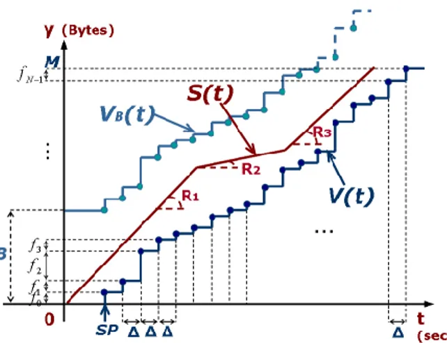
Fig. II.2 represents the playback process of an MP3 audio file by means of a graph-ical model [FR97] [Zha96] (symbols are described in Table II.1). An MP3 audio file is a sequence of frames and its playback begins at the start point (SP in the figure), which is the time when the first frame of the file is played out. Each sub-sequent frame must be played out starting at fixed, equally spaced, times called playback times. In Fig.II.2 frames are spaced by ∆ seconds.

The playback function V (t) defines the total number of bytes that must have been played out by time t in order to correctly reproduce the stream at the client. Specifically, V (t) is defined as follows:

V (t) =      0 if t < SP k P i=0 fi if t ∈ [SP +k∆, SP +(k+1)∆) (II.1)

k = 0, . . . , N − 1; i = 0, . . . , k. fi is the size in bytes of the ith _{frame in the} stream, and k is the number of the ∆-sized inter-frame spaces occurred from the starting point SP up to time t. The playback times can thus be formally defined as SP +k∆, k = 0, . . . , N −1, and are actually deadlines for frame arrivals at the client, and for frame deliveries at the proxy. During a streaming session, frames usually arrive at the client ahead of their designated playback times, and are thus temporarily stored in the client buffer, whose size will be hereafter referred to as B. As V (t) represents a lower bound for the number of bytes arrived at the client by time t, it is possible to define an upper bound for this number of bytes, denoted as VB_{(t). V}B_(t)_{is the maximum number of bytes that the client can host by time t} without causing a buffer overflow, and can thus be computed as VB_{(t) = B+V (t).}

c

(32)

Figure II.2.: Streaming model under real-time constraints: graphical model.

Table II.1.: Symbols used in the Streaming Model.

Symbol Meaning

∆ The time interval between two consecutive frames. N The number of frames in the multimedia file. fi, 0 ≤ i < N The size of the ith_{frame in the multimedia file.}

M = N−1

P i=0

fi The size of the multimedia file. B ≥ max

0≤i<Nfi The size of the client buffer. S(t) The scheduling function.

Ri The ith_{transmission rate.}

SP The Start Point: when playback begins. V (t) The playback curve.

(33)

Start Point and Sleep Time Computations 21 The scheduling function S(t) defines the number of bytes sent by the proxy to the client by time t, while the corresponding arrival function A(t) defines the number of bytes received by the client by time t. Clearly, the relation S(t) ≥ A(t) always holds, the difference between S(t) and A(t) depending on the network delay and jitter. However, it is generally assumed that S(t) = A(t) and the difference between the two curves is heuristically taken into account by slightly enlarging the size of the client buffer so as it can absorb both the jitter and the transfer delay. Therefore, hereafter we will assume S(t) = A(t). Based on this assumption, and recalling the definition of both V (t) and VB_{(t), it follows that a scheduling function is any} non-decreasing function confined between V (t) and VB_{(t), i.e., the following equation} holds:

V (t) ≤ S(t) ≤ VB(t). (II.2)

Finally, it is worth noting that the playback process extracts one single frame at a time from the client buffer at each playback time. Therefore, the level of the client buffer, at the time instant t, is the difference between the total number of bytes arrived at the client by time t, and the total number of bytes already played back, i.e., S(t)−V (t).

The scheduling algorithms define different scheduling curves depending on the particular goal targeted. When traffic smoothing is the target, the scheduling curve is a polyline with line segments of different slopes corresponding to differ-ent transmission rates (Ri is the ith _{transmission rate). In this chapter we will} use polylines that alternate line segments with zero slope (OFF periods) and line segments with non-zero slope (ON periods).

5.2. Start Point Computation

In this section we will show how the RT_PS protocol derives the start point, i.e., the initial playback delay. As a first step, it is worth focusing on constant-rate ON/OFF schedules, i.e. ON/OFF schedules where data transfers during the ON periods occur at a constant rate R. A deep analysis on constant-rate ON/OFF schedules applied to VBR traffic can be found in [Zha96] and [ZH97]. These pieces of work prove that, given the constrained region delimited by the functions

c

(34)

V (t), VB_{(t), t = 0, y = 0 and y = M (see Fig. II.2), it is possible to find an} ON/OFF schedule only in case the transmission rate is greater than a minimum value, hereafter referred to as ¯R. For some combination of V (t), VB_{(t), and M ,}

¯

Rcould be 0, meaning that the schedule is always feasible. For any R ≥ ¯R, many ON/OFF schedules can be conceived, which differ in the start point value, and the number, position and duration of the OFF periods. However, a minimum ON/OFF schedule exists among these, which is defined as R-envelope and denoted as ER(t). It was formally defined in [Zha96] and is, intuitively, the ON/OFF schedule closest to the playback curve V (t). Therefore, for any possible ON/OFF schedule SR(t) the following equation holds:

SR(t) ≥ ER(t); (II.3)

∀t, 0 ≤ t < SP +N ∆, , where N is the total number of frames composing the file, and ∆ is the time the playback process takes to play a single frame. For the sake of semplicity, hereafter we will only refer to the sequence ER[k][HHHK02] instead of the continuous function ER(t). ER[k]is composed by the samples picked up from ER(t)at regular time intervals. It can easily be obtained starting from the definition of its last sample ER[N −1]which corresponds to the end of the playout curve (M ) at the last playback time. Formally, ER[N − 1] = V (tlast_{) = M}_{, where} tlast_{= SP +(N −1)∆. Drawing from there a descending R-sloped line segment that} ends at the previous playback time (i.e., ∆s before, when t = tprev_{= SP+(N−2)∆),} the new sample ER[N−2]corresponds to the end-point of the segment, in case it is higher than the value of the playout curve V (tprev_{), or to the corresponding value} of the playout curve V (tprev₎ _{otherwise. Subsequent samples can be obtained,} again, starting from the new sample ER[N −2]and drawing a new R-sloped line segment till the previous playback time, and so on. By repeating this procedure until the time t = 0 is reached, the entire sequence ER[k] is obtained. More

(35)

Start Point and Sleep Time Computations 23 formally, ER[k]can be expressed as follows:

ER[k] = ER(SP +k∆) =      V (SP +(N −1)∆) if k = N −1 max{ER[k+1]−R∆, V (SP +k∆)} if 0 ≤ k < N −1 0 if k < 0 (II.4)

where 0 ≤ k < N and R∆ is the total number of bytes that can be transmitted during the time interval ∆ assuming a transmission rate R.

The minimum rate ¯Rthat allows an ON/OFF schedule to be performed is exactly the minimum rate for which an ER(t) curve exists inside the region defined by V (t), B, and M . Specifically, the following equation holds:

¯

R = min{R | ∃ER(t)}. (II.5)

At the beginning of the streaming session, the RT_PS proxy-side component calcu-lates the minimum rate ¯Rfor the audio sequence to be transmitted, and contrasts it with the bandwidth R0 _{available on the wireless link. The streaming process} can actually start only if R0_{≥ ¯}_R.

After this preliminary check, the RT_PS proxy component can decide the playback start point. Assuming that the proxy starts to transmit the frames at time 0, the start point corresponds to the initial delay. Obviously, a long initial delay grants more time for pre-buffering at the client and prevents the playback process from starving due to buffer underflow. However, several reasons suggest keeping the initial delay short. First, the user is not willing to wait for long time before starting to listen to the selected audio file. Moreover, as is shown in [Zha96], an increase in the initial delay causes an increase in the total idle period (i.e., the sum of all the OFF periods) while the total ON period remains unmodified. In our solution this increases the energy consumption due to the energy amount consumed by the WNIC while in the sleep mode.

The start point is calculated as follows. Given the initial transmission rate R0_{, the} minimum possible initial delay dR0 is the distance, measured on the X-axis (t),

c

(36)

between R0_{-envelope E}

R0(t) and V (t). To avoid underflowing the client buffer

due to possible variations in the available throughput, the initial delay is calcu-lated with reference to R0_/2_{-envelope instead of R}0_{-envelope, i.e., d}

R0_/2 is used

instead of dR0. The rationale behind this heuristic comes from the following

prop-erty [Zha96]. Given two transmission rates R1and R2, such that 0 ≤ R1≤ R2, the following relations hold:

ER₁(t) ≥ ER₂(t), dR₁≥ dR₂; (II.6) ∀ t, 0 ≤ t < SP +N ∆. Using dR0 would lead to buffer underflow even for small

reductions in the available throughput. On the other hand, using dR0_/2 a buffer

underflow does not occur unless the available throughput falls below R0_/2. Finally, for very low values of R0_{, the initial delay dR}

0_/2may be too long, beyond

the maximum delay the user is willing to tolerate. In this case the initial delay is taken as the maximum initial delay specified by the user.

5.3. Sleep Time Computation

The next issue to be addressed is how to compute the duration of an OFF period during which the WNIC can be switched to the sleep mode. An OFF period starts when either the client buffer fills up, or the available throughput becomes too low (half the initial value).

The procedure described above to calculate the initial delay is used to compute the durations of the OFF periods too. Let us assume that the server has just scheduled and sent to the client S(t∗₎_{bytes. Let us also assume that, according to} the last estimate provided by the client, the current transmission rate (available throughput) on the wireless link is R∗_{. Then, the maximum allowed sleep time} corresponds to the distance, measured on the y = S(t∗₎_{horizontal axis, between} S(t∗)and R∗_{-envelope E}

R∗(t). Intuitively, assuming that the throughput R∗ will

also be available in the near future, the mobile host can sleep until the scheduling function intersects ER∗(t). As above, to reduce the risk of playback starvation,

R∗/2-envelope ER∗_/2(t)is used instead of R∗-envelope E_R∗(t). Therefore, a buffer

(37)

Available Throughput Estimate 25 Obviously, an OFF period actually starts only if the calculated OFF duration is greater than the time needed to the WNIC to switch from active to sleeping and back from sleeping to active. When this condition does not hold the client buffer level is deemed to be a low water level because the scheduling function is very close to the playback curve and a transmission interruption is too dangerous. In this case, the transmission must continue even if the available throughput on the wireless channel is low. Otherwise, the client buffer level is considered safe and an OFF period can start.

6. Available Throughput Estimate

In this section we will show how the RT_PS protocol estimates the throughput available on the wireless link. The transmission rate used by the RT_PS protocol to derive the ON/OFF schedule corresponds to the estimated available throughput. It is yielded with a very simple and fast technique that guarantees good accuracy for our purposes nevertheless. In principle it works as follows. The RT_PS proxy sends a train of back-to-back packets to the RT_PS client. The packet train is pre-ceded by a special packet informing the client that a new packet train is starting. Upon receipt of the special packet the client records the time. Moreover, it starts counting the number of bytes contained in the subsequent packet train. The avail-able throughput experienced by the client is thus estimated as the ratio between the total number of bytes contained in the received packet train and the total time needed to receive those bytes (time interval between receipt of the special packet and receipt of the last packet in the train).

For an accurate estimate two key factors must be taken into account: the packet train length and the size of each single packet. In our experiments we found that the best accuracy is achieved when the packet size is 1472 bytes. This value cor-responds to the maximum UDP-payload size that does not undergo the MAC layer fragmentation (when the packets transmitted during the streaming session are shorter than 1472 bytes, the overhead times introduced for each single transmis-sion at the MAC layer -according to the 802.11b standard- have a greater impact on the total transmission time and the resulting throughput calculated). We also

c

(38)

found that, to achieve an accurate estimate the packet train should include at least 50 1472-byte packets. Under these conditions, we found that the maximum throughput experienced by the client in a Wi-Fi WLAN without any other compet-ing traffic is approximately 6.65 Mbps when the WNIC data rate is 11 Mbps, 4.04 Mbps when the data rate is 5.5 Mbps, and 1.69 Mbps when the data rate is 2 Mbps. However, in our implementation, estimates work out from the RT_PS traffic during the ON periods. Hence, a packet is an RT_PS message that includes an RTP packet. The RTP packet is further composed by couples <ADU descriptor, ADU frame> that cannot be fragmented for the sake of loss tolerance [Fin04]. This may lead to a large variability in the packet sizes and to degrading the accuracy in the estimates. To overcome this problem, the RT_PS proxy sends an integer value of couples <ADU descriptor, ADU frame> in a single RTP packet so as to keep the RT_PS packet sizes as close as possible to the ideal value (i.e., 1472 bytes). Moreover, the train length is increased from 50 to 60 packets. This is generally possible in our scenario except when the client buffer is small. In that case the accuracy in estimates slightly decreases. Fig. II.3 shows the throughput estimated on a

Figure II.3.: Available bandwidth estimates for different client buffer size and WNIC data rate.

WLAN without competing traffic, for different data rates of the WNIC and different sizes of the client buffer. These results have been obtained by using a prototype implementation of the proposed architecture (see Section 7 for details about the

(39)

Available Throughput Estimate 27 experimental testbed and the measurement methodology). Specifically, the above algorithm was used for estimating the throughput experienced by the client. The results in Fig. II.3 show that, in absence of interfering traffic, a streaming session is able to exploit up to 6.54 Mbps (instead of 6.65 Mbps) with 11 Mbps data rate, up to 4.01 Mbps (instead of 4.04 Mbps) with 5.5 Mbps data rate, and up to 1.66 Mbps (instead of 1.69 Mbps) with 2 Mbps data rate. These results show that our estimate methodology, based on real RT_PS traffic is accurate.

The client buffer size is another factor that affects the accuracy in the throughput estimates. When the client buffer is large, the RT_PS schedule produces a small number of very long OFF periods. This results in a very bursty traffic where trans-missions are concentrated in short periods separated by long interruptions. As the client buffer size decreases the number of the OFF periods increases, whereas their lengths decrease. Therefore, more control packets are needed [ACG+_05b_],

which are shorter than the packets carrying audio data. Clearly, this results in the available throughput be slightly underestimated, as highlighted in Fig. II.3. Based on the above experimental results, we can conclude that, for sufficiently large buffers, our algorithm for bandwidth estimate is accurate. Please note that, since each estimate is derived from a long train of packets, short-term variations in the available throughput are filtered out.

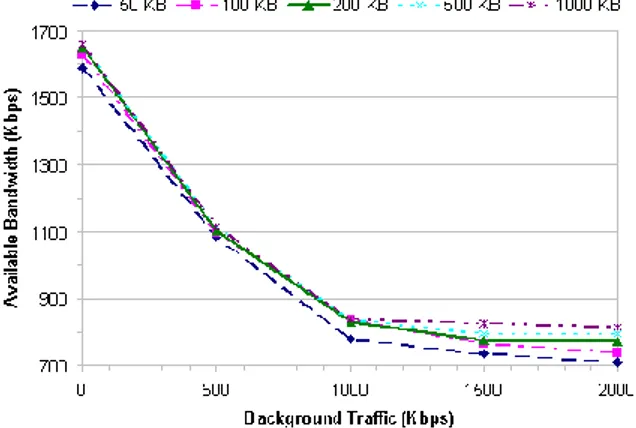
We also investigated the effect of some competing traffic on the accuracy of the estimate algorithm. When adding background traffic to the streaming flow the estimates of the available bandwidth decrease accordingly. Fig. II.4 focuses on a WNIC data rate of 2 Mbps and shows the estimated throughput for increasing rates of the background traffic and different client buffer sizes. As expected, the avail-able throughput decreases as the background traffic grows up. When the back-ground traffic is so high to saturate the wireless bandwidth both the backback-ground and the streaming traffic are expected to achieve half the maximum available bandwidth, i.e. 845 Kbps (as is stated above, the maximum available bandwidth is 1.69 Mbps when the data rate of the WNIC is 2 Mbps). Fig. II.4 shows that the throughput estimated is very close to the expected results. Again, the best accuracy is achieved with the largest client buffer size.

c

(40)

Figure II.4.: Available bandwidth estimates for different client buffer size and background traffic.

7. Experimental Evaluation

We implemented the RT_PS protocol in a prototype version of our architecture and conducted an extensive experimental analysis to evaluate its performance. In our analysis we first considered a scenario with a single streaming session from the proxy to the mobile client. Then, we also considered the more general case with multiple simultaneous streaming sessions.

We evaluated the energy efficiency of our protocol by measuring the power saving index I_ps which is the ratio between the energy consumed during the streaming session by the WNIC of the client device when the RT_PS protocol is used, and the energy consumed without the RT_PS protocol [ACGP03b], [ACGP03a]. More formally, I_ps is defined as follows:

I_ps =ERT_P S

E_RT_{_}_{P S}; (II.7)

where:

(41)

Experimental Evaluation 29 and

E_RT_{_}_{P S}= WON·(TSLEEP+TON). (II.9) In Equations II.8 and II.9 TON is the sum of all the ON periods, while TSLEEP is the sum of all the OFF periods. The power consumption of the WNIC in the active mode was approximated by a constant value, irrespective of the specific state (rx, tx, idle) the WNIC was operating in. Specifically, we considered WON= 750mW and WSLEEP= 50mW [KB02].

Finally, it should be pointed out that each experiment was replicated three times, and the results reported below are the average values over the three replicas.

7.1. Experiences with a single streaming session

In the first set of experiments we considered a single streaming session from the proxy to the client, and investigated the performance of the RT_PS protocol for different data rates of the WNIC (we manually set the WNIC to work at a constant data rate of either 2 Mbps, 5.5 Mbps or 11 Mbps during each single experiment) and different sizes of the client buffer (from 1000 KB down to 50 KB). We also analysed the impact on the performance of some background traffic.

When there is no background traffic the throughput achieved by the streaming session is maximum, and the proxy stops transmitting data to the client only when the client buffer is full. As expected, the RT_PS protocol performs better for greater data rates. This is because when the data rate is greater the data transfer is faster, and the WNIC is active for shorter time. We found that, with a WNIC data rate of 11 Mbps, I_ps is almost constant (i.e., it exhibits only a slight dependence on the client buffer size), and ranges from 8.50% (10 MB) to 8.63% (50 KB). Hence, the RT_PS protocol allows up to 91.50% saving of the energy consumed when no energy management policy is used. When the WNIC data rate decreases, the I_ps index increases, i.e., the energy saving decreases. With a WNIC data rate of 5.5 Mbps, the I_ps index ranges from 9.66% (10 MB) to 10.33% (50 KB), and with a data rate of 2 Mbps it ranges from 13.90% (10 MB) to 14.23% (50 KB). In the worst case the energy saving is greater than 85%. The above results show that the I_ps index increases as the client buffer size decreases. These variations can be

c

(42)

Figure II.5.: I_ps experienced by a streaming flow competing with CBR back-ground traffic. Min burstness: 1 packet per single burst.

explained as follows. As anticipated in Section 6, when the buffer size decreases the following side effects occur: i) the amount of control traffic increases, ii) the accuracy of the estimator of the available bandwidth decreases, and iii) the schedule is characterized by a greater number of shorter ON periods. Due to i) the WNIC consumes more energy because is active for longer time to support the increased control traffic. Moreover, since for small buffer sizes the estimator tends to underestimate the available bandwidth, the WNIC remains active for much more time in order to prevent buffer underflows. Finally, a greater number of short ON periods in the transmission schedule contributes to increase the energy consumed in frequently switching the WNIC on and to sleep mode.

To investigate the impact of the interfering traffic on the protocol performance we introduced an additional mobile host sending CBR (Constant Bit Rate) traffic, i.e., a periodic flow of UDP packets, to the proxy. We tested our system in the worst case, i.e., with a WNIC data rate of 2 Mbps. Fig. II.5 summarizes the results obtained from the experiments with the background CBR traffic. It clearly emerges that I_ps increases when the amount of background traffic increases, thus leading to a higher energy consumption. This is because the streaming session experiences a lower throughput and the WNIC must be active for longer time since the client

(43)

Experimental Evaluation 31

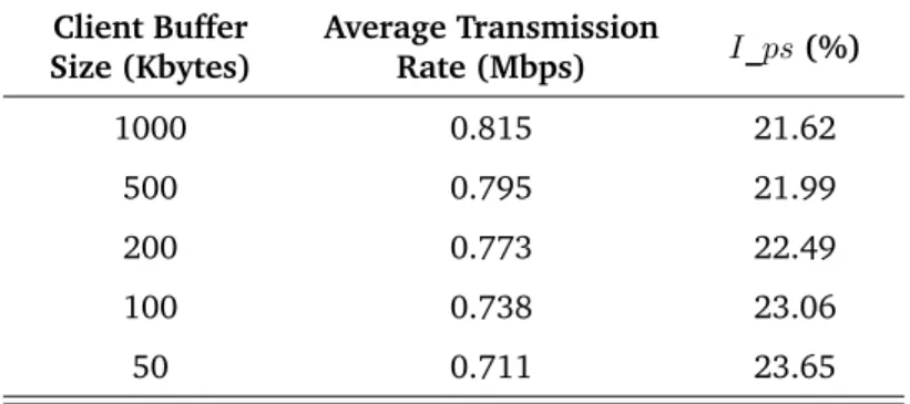
Table II.2.: I_ps vs. Client Buffer Size. Worst Case: 2 Mbps Data Rate, 2 Mbps Background Traffic. Client Buffer Size (Kbytes) Average Transmission Rate (Mbps) I_ps (%) 1000 0.815 21.62 500 0.795 21.99 200 0.773 22.49 100 0.738 23.06 50 0.711 23.65

buffer fills up slowly and the risk of playback starvation is higher. When the rate of the background flow increases beyond 845 Kbps the wireless bandwidth is almost equally shared between the streaming flow and the CBR flow, i.e., the throughput experienced by the streaming session is approximately constant (845 Kbps is half of the maximal bandwidth, 1.69 Mbps, experienced with 2 Mbps data rate). Therefore, for a given buffer size, I_ps tends to flatten. Table II.2 shows the performance of the RT_PS protocol in the worst conditions, i.e., when the rate of the background traffic is 2 Mbps and, hence, the interfering mobile host has always a packet ready for transmission. I_ps is, at most, equal to 23.65% which corresponds to an energy saving of 76.35%.

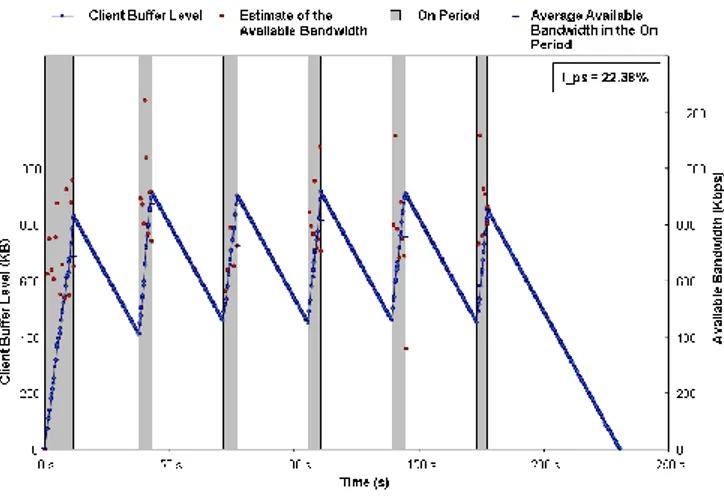
To conclude our analysis on the impact of the background traffic, we now show the evolution over time of the following parameters: client buffer level, ON and OFF durations, and estimated bandwidth. Fig. II.6 shows the system behavior when there is no background traffic, while Fig. II.7 shows the same behavior when the background traffic is maximum. Fig. II.6 shows that the estimated bandwidth (the dots inside the ON periods) is high because there is no interfering traffic, and the buffer level grows up until the buffer becomes full. During the OFF periods the playback process consumes data in the client buffer at a constant rate and the buffer level decreases linearly. In Fig. II.7 the bandwidth estimated is lower be-cause of the background traffic. Therefore, the buffer level during the ON periods

c

(44)

Figure II.6.: Variations in the client buffer level during the streaming session. The client buffer size is 1000 KB. No background traffic is present.

Figure II.7.: Variations in the client buffer level during the streaming session. The client buffer size is 1000 KB. Maximal background traffic is present.