Design, calculation and simulation of a wind tunnel for calibration of hot wire probes

(1)

Alma Mater Studiorum

Universitá di Bologna

SCHOOL OF ENGINEERING AND ARCHITECTURE

Forlì Campus

Second Cycle Degree in

INGEGNERIA AEROSPAZIALE/ AEROSPACE NGINEERING

Class LM-20

THESIS

In Fluid Dynamics, ING-IND/ 06

Design, calculation and simulation of a wind tunnel for calibration of hot wire

probes

Student: FORNERO, Agustin Supervisor: Ing. BELANI, Gabriele. Year: 2018

(2)

Content

List of Figures ... 4 List of Tables ... 6 Introduction: ... 9 Hot-wire ... 11 Introduction ... 11 Equations ... 12 Types of Probes ... 13 Calibration ... 14 Types ... 17

Constant current anemometer ... 17

Constant temperature anemometer ... 18

Wind tunnels ... 19

Introduction ... 19

Design criteria ... 22

Definition of the elements of the wind tunnel ... 22

Power plant ... 22

Honey Comb ... 23

Screens ... 23

Contraction “cone” or nozzle ... 24

Component energy losses ... 28

Introduction ... 28

Screens ... 29

Honeycombs ... 31

Jet power ... 33

Calculation of the coefficient losses. ... 35

Power in the test section ... 35

Screen losses ... 36

Honeycomb Losses ... 37

Power Needed ... 39

Map of fan usage ... 39

Convergent ... 42

Designs of the convergent ... 42

(3)

Convergent ... 44 Simulations ... 47 Introduction ... 47 Results ... 49 25 Degrees Contraction ... 49 40 Degrees Contraction ... 51 Convergent Design ... 53

25 Degrees Contraction with Extension ... 55

40 Degrees with extension ... 57

Analysis ... 59

Comparison ... 60

Comparison of the pressure along the wall for the options ... 60

Velocity distribution in test-section ... 61

Analysis ... 63

Comparison between the best options... 63

Pressure... 63

Velocity Distribution ... 65

Analysis ... 67

Model of the Wind tunnel ... 68

Fan Selection ... 69

Conclusion ... 70

Bibliography ... 71

Appendix ... 72

Appendix A: Components Dimensions ... 72

(4)

List of Figures

Figure 1 Different types of probes (Reprinted from Jorgensen (2002)) ... 14

Figure 2 Example of a calibration plot for the X-wire probe (Reprinted from Orlu [9]) ... 16

Figure 3 Example of a constant current anemometer circuit ... 18

Figure 4 Example of a constant temperature anemometer circuit ... 18

Figure 5 Different types of honeycombs designs (Reprinted from [2]) ... 23

Figure 6 Mesh example ... 30

Figure 7 Hexagon example ... 32

Figure 8 Example of a honeycomb cell ... 33

Figure 9 Curve of usage of the fan ... 40

Figure 10 25 Degrees contraction model ... 42

Figure 11 40 Degrees Contraction model ... 43

Figure 12 25 Degrees contraction with extension model ... 43

Figure 13 40 Degrees contraction with extension model ... 44

Figure 14 Example to calculate length of contraction ... 44

Figure 15 Shape of the convergent ... 46

Figure 16 Convergent model ... 46

Figure 17 Graph of pressure for 0.2 m/s for the 25 Degrees contraction with the pressure in the y axis in [PA] and the position in the contraction in [m] along the x-axis for the wall (values of position given by ANSYS due to the positioning of the model). ... 49

Figure 18 Graph of velocity for 0.2 m/s for the 25 Degrees contraction with the position in the test-section in the y axis in [m] and the velocity of each point in the x axis in [m/s]. (Values of position given by ANSYS due to the positioning of the model) ... 49

Figure 19 Graph of pressure for 10 m/s for the 25 Degrees contraction with the pressure in the y axis in [PA] and the position in the contraction in [m] along the x-axis for the wall (values of position given by ANSYS due to the positioning of the model). ... 50

Figure 21 Graph of pressure for 0.2 m/s for the 40 Degrees contraction with the pressure in the y axis in [PA] and the position in the contraction in [m] along the x-axis for the wall (values of position given by ANSYS due to the positioning of the model). ... 51

Figure 23 Graph of pressure for 10 m/s for the 40 Degrees contraction with the pressure in the y axis in [PA] and the position in the contraction in [m] along the x-axis for the wall (values of position given by ANSYS due to the positioning of the model). ... 52

(5)

Figure 24 Graph of velocity for 10 m/s for the 40 Degrees contraction with the position in the test-section in the y axis in [m] and the velocity of each point in the x axis in [m/s]. (Values of position given by ANSYS due to the

positioning of the model) ... 52 Figure 25 Graph of pressure for 0.2 m/s for the Convergent design with the pressure in the y axis in [PA] and the position in the contraction in [m] along the x-axis for the wall (values of position given by ANSYS due to the

positioning of the model). ... 53 Figure 26 Graph of velocity for 0.2 m/s for the Convergent design with the position in the test-section in the y axis in [m] and the velocity of each point in the x axis in [m/s]. (Values of position given by ANSYS due to the positioning of the model) ... 53 Figure 27 Graph of pressure for 10 m/s for the Convergent design with the pressure in the y axis in [PA] and the position in the contraction in [m] along the x-axis for the wall (values of position given by ANSYS due to the

positioning of the model). ... 54 Figure 28 Graph of velocity for 10 m/s for the Convergent design with the position in the test-section in the y axis in [m] and the velocity of each point in the x axis in [m/s]. (Values of position given by ANSYS due to the positioning of the model) ... 54 Figure 29 Graph of pressure for 0.2 m/s for the 25 Degrees contraction with the extension with the pressure in the y axis in [PA] and the position in the contraction in [m] along the x-axis for the wall (values of position given by ANSYS due to the positioning of the model). ... 55 Figure 30 Graph of velocity for 0.2 m/s for the 25 Degrees contraction with the extension with the position in the test-section in the y axis in [m] and the velocity of each point in the x axis in [m/s]. (Values of position given by ANSYS due to the positioning of the model). The velocity is shown in different sections of the extension (beginning, middle and end). ... 55 Figure 31 Graph of pressure for 10 m/s for the 25 Degrees contraction with the extension with the pressure in the y axis in [PA] and the position in the contraction in [m] along the x-axis for the wall (values of position given by ANSYS due to the positioning of the model). ... 56 Figure 32 Graph of velocity for 10 m/s for the 25 Degrees contraction with the extension with the position in the test-section in the y axis in [m] and the velocity of each point in the x axis in [m/s]. (Values of position given by ANSYS due to the positioning of the model). The velocity is shown in different sections of the extension (beginning, middle and end). ... 56 Figure 33 Graph of pressure for 0.2 m/s for the 40 Degrees contraction with the extension with the pressure in the y axis in [PA] and the position in the contraction in [m] along the x-axis for the wall (values of position given by ANSYS due to the positioning of the model). ... 57 Figure 34 Graph of velocity for 0.2 m/s for the 40 Degrees contraction with the extension with the position in the test-section in the y axis in [m] and the velocity of each point in the x axis in [m/s]. (Values of position given by ANSYS due to the positioning of the model). The velocity is shown in different sections of the extension (beginning, middle and end). ... 57 Figure 35 Graph of pressure for 10 m/s for the 40 Degrees contraction with the extension with the pressure in the y axis in [PA] and the position in the contraction in [m] along the x-axis for the wall (values of position given by ANSYS due to the positioning of the model). ... 58 Figure 36 Graph of velocity for 10 m/s for the 40 Degrees contraction with the extension with the position in the test-section in the y axis in [m] and the velocity of each point in the x axis in [m/s]. (Values of position given by ANSYS due to the positioning of the model). The velocity is shown in different sections of the extension (beginning, middle and end). ... 58

(6)

Figure 37 Comparison between the different options in pressure for 0.2 m/s. Each pressure graph was

adimensionalized respect to the last point in the x-axis and respect to the highest pressure in the y-axis for each model. ... 60 Figure 38 Comparison between the different options in pressure for 10 m/s. Each pressure graph was

adimensionalized respect to the last point in the x-axis and respect to the highest pressure in the y-axis for each model. ... 60 Figure 39 Comparison between the different options of velocity for 0.2 m/s. Each velocity graph is adimensionalized in the velocity (x-axis) respect to the highest velocity encountered in the middle of the test-section. Position is not adimensionalized since every graph has the same one. ... 61 Figure 40 Graph of velocity for 0.2 m/s of the convergent for comparison. Velocity in the x-axis is adimensionalized respect of the highest velocity encountered in the middle of the test-section. Position in the y-axis is

adimensionalized respect the highest position of the test-section. (Given by ANSYS by the positioning of the model). ... 61 Figure 41 Comparison between the different options of velocity for 10 m/s. Each velocity graph is adimensionalized in the velocity (x-axis) respect to the highest velocity encountered in the middle of the test-section. Position is not adimensionalized since every graph has the same one. ... 62 Figure 42 Graph of velocity for 10 m/s of the convergent for comparison. Velocity in the x-axis is adimensionalized respect of the highest velocity encountered in the middle of the test-section. Position in the y-axis is

adimensionalized respect the highest position of the test-section. (Given by ANSYS by the positioning of the model). ... 62 Figure 43 Comparison between the best two options in pressure for 0.2 m/s. Each pressure graph was

adimensionalized respect to the last point in the x-axis and respect to the highest pressure in the y-axis for each model. ... 63 Figure 44 Comparison between the best two options in pressure for 10 m/s. Each pressure graph was

adimensionalized respect to the last point in the x-axis and respect to the highest pressure in the y-axis for each model. ... 64 Figure 45 Graph for comparison of velocity for 0.2 m/s for the 25 Degrees contraction(1st_{best option).the graph is}

adimensionalized in the velocity (x-axis) respect to the highest velocity encountered in the middle of the

test-section. Position is not adimensionalized since it’s not needed. ... 65 Figure 46 Graph of velocity for 0.2 m/s of the convergent for comparison(2nd_{best option. Velocity in the x-axis is}

adimensionalized respect of the highest velocity encountered in the middle of the test-section. Position in the y-axis is adimensionalized respect the highest position of the test-section. (Given by ANSYS by the positioning of the model). ... 65 Figure 47 Graph for comparison of velocity for 10 m/s for the 25 Degrees contraction(1st_{best option).the graph is}

adimensionalized in the velocity (x-axis) respect to the highest velocity encountered in the middle of the

test-section. Position is not adimensionalized since it’s not needed. ... 66 Figure 48 Graph of velocity for 10 m/s of the convergent for comparison(2nd_{best option. Velocity in the x-axis is}

adimensionalized respect of the highest velocity encountered in the middle of the test-section. Position in the y-axis is adimensionalized respect the highest position of the test-section. (Given by ANSYS by the positioning of the model). ... 66 Figure 49 Exploded model of wind tunnel ... 68 Figure 50 Model of Wind tunnel ... 69

(7)

(8)

List of Tables

Table 1 Specifications of screens used ... 36

Table 2 Porosity for each screen ... 37

Table 3 Values for calculation of coefficient loss ... 37

Table 4 Coefficient loss for each screen ... 37

Table 5 Specifications for the honeycomb used ... 37

Table 6 Reynolds number and landa coefficient... 38

(9)

Introduction:

Anemometry is the process of ascertaining the speed, and direction of wind in an airflow. To do this it requires the use of a device, called anemometer. The anemometer is an instrument used to measure the speed of any gas. There are many different types of anemometers but the most common for aeronautics and aerodynamics use is hot wire anemometry.

Hot wire anemometry measures both speed and pressure of the airflow under the principle that a heated body, in this case a fine wire, placed in a flow will experience a cooling effect. This effect is mainly associated to forced convection heat losses which are strongly velocity dependent. If it’s possible to measure this heat loss, then it’s possible to retrieve the flow velocity based on the wire’s cooling rate. In the hot-wire case this cooling effect can be measured either by measuring the change in the temperature of the sensor (constant current anemometer) or either by measuring the action necessary to keep it at a constant temperature (constant temperature anemometer). The hot wire is made of platinum or tungsten and they range in length between 0.5 and 2 mm and in diameter from 0.6 to 5 microns.

It comes in a single-wire configuration or with two or more wires configuration depending on the application is being used and the purpose of it.

In the constant current anemometer, the hot wire is supplied with a constant current and inserted in a Wheatstone bridge where is kept on balance, later by the equation of Wheatstone bridge the resistance of the wire is retrieved and knowing the current, which is constant, we can calculate the speed of the airflow. In the other method, constant temperature anemometer, the wire is kept in a constant temperature (and therefore resistance), so it measures in a faster way and with a faster response.

The Center for International Collaboration on Long Pipe experiments of the Bologna University, CICLoPE, located in predappio, for the long Pipe wind tunnel. The purpose of CICLoPE is focused on the research of turbulence for High Reynolds number. The CICLoPE wind tunnel ensures a size of the smallest scale of the turbulent boundary layer that is sufficiently large to be resolved with the actual measurement techniques for High Reynolds number. To perform these measurements the hot-wire probes, specially X-probes with two wires to measure two components of the velocity, are used.

Like every other measure instrument, the hot wire needs to be calibrated to have an accurate reading of the speed of the airflow, especially this type of anemometer since it can be affected by contamination and their response is highly dependent on ambient quantities. The calibration is achieved by establishing the relationship between the anemometer output voltage and the magnitude and direction of the incident velocity vector, each hot wire must be calibrated before measurements by exposing it to a set of known velocities and then a calibration curve must be fitted to the calibration points.

The exposition to the set of known velocities is achieved in a calibrating wind tunnel, which is a “blower tunnel” who is designed to have a most laminar possible flow in the open test section to get the most accurate reading of the velocity and it has the possibility to achieve different speeds to make possible the calibration of the probes.

(10)

The design of this kind of tunnel is performed to meet the investigation purposes, where the parameters of velocity, dimensions and the uniformity of the flow are set. Then comes the calculation of the power lading factor to maintain these parameters and flow characteristics in the test section. Once this is obtained, the elements that will get the flow to these characteristics needs also to be designed and calculate their pressure losses to know how much power we will need to run the tunnel. The pressure loss for each component depends in the geometry and functionality of it.

Once all components are designed and selected, a model representing the wind tunnel can be made to show how it will work and how the components will be placed and kept there. It can also be done the selection of the power plant that will power the wind tunnel.

The present thesis will be focused on the design and selection of the components for a wind tunnel that will be used to calibrate the probes used in CICLoPE. Inside these components, a comparison between different convergent will be made to select the one who will fit the best this application. It will also select the power plant for this and present a model for a future construction of it.

The specifications prior to the design for the wind tunnel are:

1. The flow in the test-section should be as uniform as possible. A difference of less than 0.5% in the velocity distribution in the test-section is required to achieve a calibration the most accurate possible.

2. The test section will have 10mm height by 500mm wide.

3. The settling chamber where the components to achieve the flow characteristics will have 50mm height by 500mm wide. The length of the settling chamber is not yet defined, it will be defined by the number of components since it will be a separation of 15cm between them for stabilization of the flow.

4. The contraction to the test-section is only in height not in wide making it a two-dimensional contraction. Several options will be tested to find the best solution.

This tunnel is an important one since it says before will calibrate the probes for CICLoPE that allows the research performed there, that’s the main reason the flow characteristics of the test-section have high requirements, to ensure a proper functioning that will ensure realistic and accurate results in the research performed at this center.

In the next pages, added to the stated before, an explanation of the functioning of the probes and the calibration method will be written along with an introduction to wind tunnels and the different components of one.

(11)

Hot-wire

Introduction

Hot-wire anemometry is the leading technique for velocity measurements in the field of turbulent flows, because with a careful design of the sensor and anemometer system, it can achieve and spatial and temporal resolution far much better than the other measurements techniques, making it an invaluable tool for turbulence investigation. It relies on the fact that the electrical resistance of a metal conductor is a function of its temperature. The essential part of the hot-wire anemometer is, therefore, a miniature metal element, heated by an electrical current and inserted into the flow under investigation. When inserted into the flow it experiences a cooling effect; this effect is mainly associated to forced convection heat losses which are strongly velocity dependent. The transfer of the heat from the element increases with increasing flow velocity in the neighborhood of the element, if we can measure this heat loss, it would be possible to retrieve the flow velocity based on the wire’s cooling ratio. To get results that can be trust we need to calibrate the wires with the sensors. There are two methods to measure the cooling effect, either by measuring the chance in temperature of the sensor (constant current anemometer) or by measuring the action necessary to keep it at a constant temperature (constant temperature anemometer).

The popularity of the hot-wire anemometry is mainly because of the advantages of the process: • The sensitive is small enough not to introduce any disturbance in the flow; although the other

parts of the probe may not so it can disturb the flow in the vicinity of the wire.

• The hot-wire anemometer responds almost instantaneously to rapid fluctuations so that high-frequency effects can be recorded without distortion.

• Thanks to its very small physical dimensions, it has a small measuring volume and therefore an extremely good spatial resolution.

• The electrical signal produced by the hot-wire anemometer can be readily statically processed, both by analog and digital systems.

Even though all these advantages, there also a few drawbacks of this type of anemometer; few of those being:

• Hot-wires are limited to low and medium intensity turbulence flows, because they can’t recognize a reverse flow in a high turbulence flow due to the velocity vector may be falling outside the acceptance cone.

• They have consistent drift over time, may be affected by contamination and their response is highly dependent on ambient quantities. For this, frequent calibrations are necessary.

• Hot-wires are intrinsically fragile due to their small size, so extreme precaution while handling the probes is needed.

(12)

The wires range between 0.5 to 2 mm in length and in diameter from 0.6 to 5 microns. Tungsten, platinum or platinum-iridium wires are the most frequently used materials. They can be found hot-wires probes in different configurations, with one, two or more sensor hot-wires.

This section will provide a general description of the methods; the equations ruling the cooling effect and a brief explanation of different types of probes and the way to calibrate them.

Equations

The sensor heated by the electrical current gives up its heat to the flow into which it’s inserted by conduction, by free and forced convection, and by radiation. The last component is, however, relatively small and can be neglected.

In case of a cylinder shaped-body, like a wire, the forced convection coefficient ℎ can be expressed as:

ℎ = 𝑁𝑢𝑘𝑓 𝑑_𝑤

where 𝑘𝑓 is the thermal conductivity of the fluid, and 𝑑𝑤 is the cylinder’s diameter, in this case, the

wire. 𝑁_𝑢 is the Nusselt’s number, which it’s a function of many parameters. 𝑁_𝑢 = 𝑁_𝑢 (𝑀, 𝑅𝑒, 𝐺𝑟, 𝑃𝑟, 𝛾,𝑇𝑤− 𝑇𝑎

𝑇_𝑎 )

Which are the Mach, Reynolds Grashof and Prandtl numbers, the ratio between specific heat at constant pressure and volume, and the wire temperature difference.

If we confine our attention to incompressible flows and ignore frequency spectra and space-time correlations of temperature and velocity fluctuations in the immediate neighborhood of the sensor, we can exclude the Mach number from the dimensionless ratios. In subsonic flows, 𝛾 and 𝑃𝑟 can be considered

constant and, if the heat exchange is dominated by forced convection, which is the case for hot-wires, even the dependency on the Grashof number can be neglected. It’s good to point that the Reynolds number significant for the Nusselt number is the one of the wire. Taking all this in consideration the equation for the Nusselt number becomes:

𝑁_𝑢 = 𝑁_𝑢 ( 𝑅𝑒_𝑤,𝑇𝑤− 𝑇𝑎 𝑇_𝑎 )

The heat transfer depends on only these two dimensionless parameters. Different workers have obtained different empirical functions for the Nusselt number, and they usually share the form, for wires;

𝑁𝑢 = 𝐴1+ 𝐵1𝑅𝑒𝑤𝑛

Where A, B and 𝑛 (which for most of these functions is 0.5) are characteristic constants of the particular correlation function. Considering a specific wire diameter, 𝑅𝑒𝑤 can be considered only a function

(13)

𝑁𝑢 = 𝐴2 + 𝐵2𝑈𝑛

The heating in the wire is achieved by means of Joule effect: a current 𝐼𝑤 is passed through the wire,

and the heat liberated is equal to 𝐼𝑤2𝑅𝑤, where 𝑅𝑤 is the wire’s electrical resistance. The amount of heat

transferred to the flow at temperature 𝑇𝑎 from a hot wire, heated uniformly to a temperature 𝑇𝑤 is,

𝑄 = (𝑇_𝑤− 𝑇_𝑎) 𝐴ℎ(𝑈)

Where A is the surface area over which forced convection takes place, and ℎ is the forced convection heat transfer coefficient which is dependent, among other things, on the fluid velocity normal to the wire. Assuming equilibrium heat transfer we obtain:

𝐼_𝑤2𝑅_𝑤 = (𝑇_𝑤− 𝑇_𝑎) 𝐴ℎ(𝑈)

The change in the resistance of the wire is approximately proportional to the corresponding change in temperature, we can replace the temperature difference by a quantity proportional to the resistance difference and then combine this equation with the equilibrium equation and introduce them in the Nusselt equation to obtain the working formula relating the electrical quantities to the flow velocity,

𝐼𝑤2𝑅𝑤

𝑅_𝑤 − 𝑅_𝑎 = 𝐴 + 𝐵𝑈

𝑛

Considering the voltage across the hot-wire, 𝐸𝑤 = 𝐼𝑤𝑅𝑤 and using the proportional relation

between the temperature and resistance the equation becomes, 𝐸_𝑤2

𝑅_𝑤 = (𝐴 + 𝐵𝑈

𝑛_)(𝑇

𝑤 − 𝑇𝑎)

Types of Probes

There are different types of probes with the distinction of how many wires they have and because of that, how many components of the velocity they can measure.

The main configuration is a single wire probe, but in the Ciclope lab the most used ones are two-wire probes to use in the research of velocity fluctuations near the wall of the tunnel.

Single wire probes consist in a single wire mounted in two prongs that keep it in place. It’s placed perpendicular to the flow direction and the prongs parallel to it. It is used for uni-directional flows because it can’t determine the orientation of the velocity vector.

To carry out two velocity measurements it can be with a single wire inclined relative to the mean-flow direction, but this can only provide a statistical information of the velocity field, because of this, two-wire probes, with the two-wires placed in a X configuration is used. This probe enables simultaneous measurements of two velocity components. Depending on the application the configuration of the X-probe can vary, depending on the probe-stem orientation. It can have the sensor plane (plane where both wires are lying) parallel to the probe-stem or the sensor plane perpendicular to the probe-stem. Both wires are separated from each other in the direction normal to the sensor plane to reduce aerodynamic and thermal interferences.

(14)

Another type of two-wire probe is the v-probe, this one is used for measurements close to the wall and the special resolution in the transversal direction to the wall is of extreme importance. Both wires are placed next to each other instead of one over the other.

Figure 1 Different types of probes (Reprinted from Jorgensen (2002))

Calibration

We must note that the previous equations are practically never used to calculate the response of the hot-wire anemometry to the flow velocity. They are used only for approximate estimates of the effect of different factors on heat transfer between the wire and the flow.

The aim for the calibration procedure for a hot-wire sensor and its anemometer is to establish the relationship between the anemometer output voltage and the magnitude and direction of the incident velocity factor. Each hot-wire probe must be calibrated before measurements by exposing it to a set of known velocities. To obtain the transfer function that converts voltage data into velocities, a calibration curve must be fitted to the calibration points. Typical calibration curves include king’s law,

𝐸2 = 𝐴 + 𝐵𝑈𝑛

But also, polynomial fitting might be used, being a very common one the fourth order polynomial relation.

𝑈 = 𝐶0+ 𝐶1𝐸 + 𝐶2𝐸2+ 𝐶3𝐸3 + 𝐶4𝐸4

Despite not having any physical basis, polynomial fitting allows for a very high accuracy with a small linearization error. It works very well when high number of calibration points have been acquired but falls short when the velocities are outside of the calibration ones, i.e. low velocities. For this, King’s law remains

(15)

a better solution, because it utilizes Newton’s law of cooling that relates Joule heating and forced convection. But it also may lead to some error when forced convection is not the sole phenomenon causing cooling on the wire, for example, in very low velocities, where natural convection becomes relevant.

This is valid when the velocity vector is perpendicular to the wire and parallel to the prongs. If it’s not the case because the probe is misaligned, or the calibration also covers when the probe has an angle respect to the velocity of the flow appears an effective velocity 𝑉_𝑒 that goes into the king’s law.

𝐸2 _{= 𝐴 + 𝐵𝑉} 𝑒𝑛

This one is related to the velocity vector, V. The velocity vector can be expressed in terms of its magnitude 𝑉̅, the yaw angle 𝛼, and the pitch angle 𝛽, or in terms of the corresponding three velocity components, 𝑈𝑁(normal and in plane with the prongs), 𝑈𝑇(tangencial to the wire) and 𝑈𝐵 (binormal; normal

to the sensor and the plane of the prongs). the wire doesn’t have the same response to the three velocity components; if it has the same response the effective velocity would be equal to the magnitude of the velocity vector. However, this doesn’t occur so because of that the effective velocity is defined with the Jorgensen’s relation [3], which take these factors into account and is,

𝑉_𝑒2 _{= 𝑈}

𝑁2 + 𝑘2𝑈𝑇2+ ℎ2𝑈𝐵2

Where k and h are referred as the sensor’s yaw and pitch coefficients. And are experimentally determined weighing factors that depends mostly in the aspect ratio of the sensor.

Introducing the effective velocity in the King’s law, it’s obtained, 𝐸2 = 𝐴 + 𝐵(𝑈_𝑁2+ 𝑘2𝑈_𝑇2+ ℎ2𝑈_𝐵2)𝑛/2

Which represents a hot wire response equation considering angles between the probe and the direction of the flow.

When calibrating X-probes an angular calibration of each wire with respect to its yaw angle is needed in addition to the velocity calibration. This is usually done by placing the probe in a rotating arm while keeping the hot-wires centered and in the same measurement area.

The result will be the calibration map of the probe, and from that can be obtained the calibration curve for each of the wires using the relations written before.

The aim of the calibration is to determine the values of the constants of the previous equation. The calibration is performed in a special calibration facility or in a flow field in which the magnitude and direction of the flow vector is known.

As a rule, whether which response equation is selected, it should provide a good approximation to the calibration data over the complete range, and if required, the yaw and pitch range.

(16)

Figure 2 Example of a calibration plot for the X-wire probe (Reprinted from Orlu [9])

This way of calibrating the probes is preferred to computational procedures for the following reasons: • The basic relationship for the Nusselt number is only an approximation to the experimental

results, which always exhibit a certain spread.

• The Reynolds number is always subject to an error that cannot be controlled since the diameter of the wire is not known with absolute precision and may vary along its length. • The physical properties of a thin metal wire are always some-what different from the

properties of the corresponding material in bulk, so that tabulated data on the resistance as a function of temperature are also subject to some uncertainty.

Due to the nature of the physical principles upon which the hot-wire anemometer is based, it’s clear that is very sensitive to the temperature of the ambient. The readings will be different for a given flow velocity if the temperature of the flowing material is different, therefore, the temperature of the flowing fluid must be kept constant during the calibration measurements, and it also needs to be noted in the calibration curve the temperature at which those measurements were taken.

If a hot-wire is used to measure velocity at a higher or lower flow temperature than its calibration, the heat dissipated via forced convection will be lower, and so will be the velocity reading. To retrieve the correct velocity a compensation for temperature variations must be required.

(17)

The calibration is made at a certain temperature (𝑇𝑟𝑒𝑓), and an analytical correction must be used to

retrieve the correct voltage output at the operating flow temperature 𝑇𝑎,

𝐸(𝑇_𝑟𝑒𝑓)2 = 𝐸(𝑇_𝑎)2𝑇𝑤 − 𝑇𝑟𝑒𝑓

𝑇_𝑤 − 𝑇_𝑎

Where 𝑇𝑤 is the wire’s temperature and its fixed if the sensor is operating in constant temperature

mode, 𝐸(𝑇𝑎) is the output voltage and 𝐸(𝑇𝑟𝑒𝑓) is the compensated output voltage. This can be rewritten by

using the overheat ratio 𝑎𝑤, which is the relative difference in resistance between the wire at operating and

ambient temperature, and the temperature coefficient of electrical resistivity 𝛼, 𝐸(𝑇_𝑟𝑒𝑓)2 = 𝐸(𝑇_𝑎)2_{(1 −}𝑇𝑤− 𝑇𝑟𝑒𝑓

𝑎_𝑤/𝛼 )

−1

These parameters are known from the material properties and the anemometer’s settings and are more easily to read and use than the wire’s temperature. To employ this correction method is necessary to measure the flow temperature both during the calibration and the experiment. Since the measured average velocity always depends, at least to some extent, on the intensity of the turbulence fluctuations, the calibration measurement must be performed in a flow with the minimum possible level of turbulence, hence, the most laminar possible.

The most typical case of an increase in the air temperature in wind tunnel is connected with its heating due to the operation of the system producing the flow. For this reason, anemometer measurements on turbulence in wind tunnels must be performed only after a certain interval of time running the wind tunnel to achieve steady-state thermal conditions in the tunnel. During calibration, another probe; most of the time a Prandtl probe; is used to measure the velocity for reference.

Types

Mainly in hot-wire anemometry two types of circuits are used, constant current anemometer and constant temperature anemometer.

Constant current anemometer

It was the first mode of operation to be employed. The most practical and effective way to use this technique is to insert the sensor in a Wheatstone bridge, even though it’s not necessary. After a specific overheat ratio has been selected, the wire resistance 𝑅_𝑤 can be retrieved when the bridge is in balance by the expression,

𝑅_𝑤+ 𝑅_𝐿 𝑅1

= 𝑅3 𝑅2

Where 𝑅3 is the adjustable resistance and 𝑅𝐿 is the cable resistance, which includes also connections

and prongs resistance, with exception of the wire itself. During calibration, the current is kept at a constant value and the bridge is kept in balance by acting on the adjustable resistance; when is balanced, the 𝑅𝑤 is

(18)

Figure 3 Example of a constant current anemometer circuit

Constant temperature anemometer

This mode has become more popular later than the previous, but it presents many advantages and is currently the method universally used for turbulent velocity measurements.

Figure 4 Example of a constant temperature anemometer circuit

Since the wire is kept at a constant temperature and therefore resistance, it’s thermal inertia doesn’t limit anymore the frequency response of the system, allowing for a much better tracking of the high frequency turbulent fluctuations. However, this requires a more complex circuit that allows for extremely fast variations in the heating current of the wire; it also requires a feedback mechanism. Even though it has been theorized since the 40s it wasn’t until mid-60s when the progress in electronics allowed this mode of operation to be used. The hot-wire is placed in a Wheatstone bridge; as the flow velocity varies, the wire’s temperature varies, and so does its resistance 𝑅𝑤. The voltages 𝑒1 and 𝑒2 are the inputs of the differential

amplifier, and their difference is a measure of how much the wire’s resistance has changed. The output current of the amplifier is inversely proportional to 𝑒2 − 𝑒1, and is fed on the top of the bridge, restoring

(19)

Wind tunnels

Introduction

Since the first days of aeronautics research and developments, all have been based in the latest technologies available at the moment and all pertinent sources. Three broad categories are commonly recognized: analytical computational and experimental.

The analytical approach plays a vital role in the background studies and in gaining knowledge and setting ground information and stablishing the laws that rules the natural phenomenon when it comes to researching in aeronautics, but it never suffices for a development program of any kind. All development from the first flight of the Wright brothers to the 1960s were based on a combination of analytical and experimental approaches.

In the 1960s the evolution of electronics and computers reached a point where it was possible to use these tools to approximate solutions for forms of fluid dynamic equations (Navier-Stokes) to vehiclelike geometries. This advance and the development of methods and computing machinery advancing rapidly led to the prediction that “computer will replace wind tunnels”. However, this was not certain due to the fact that the continuing development of computers, increase in velocity and processing power and even more optimized methods to solve the fluid dynamic equations, has only partially tamed the complexity of real flows. Mainly due to turbulence that in order to achieve good results, a “turbulence model” needs to the tailored for specific types of flow, there’s no general form that is accepted for all of them.

For increasing the effectiveness of applications of the computer, Hammond[1] gives three aspects of development as pacing items: central processing speed, size of memory available and turbulence models. The first two continue to advance at a rapid rate, and the last one has had many developments but there’s not a certainty that progress in achieving generality has been made. This is the Achilles heel of current efforts to extend applications of computational dynamics.

For these reasons, the experimental brand is still today a major tool to research and develop programs in aeronautics, specially wind tunnels with contribution of computers; these are used to manage data gathering and presentation and possibly provide control of the experiment. With computers, the time required to present the corrected data in the way needed is usually less than a second after the measurement is taken.

The availability of increased computing power has contributed in other ways to the effectiveness of wind tunnels programs; the process of model design and construction has been affected by the use of computer-design, which provides a way to make designs easily and in a fast way and the possibility of changes in them without losing time in the process. This can shorten the time required to prepare for an experiment or an eventually change of the purpose of the wind tunnel during the phase design.

Wind tunnels, especially low speed wind tunnels, are devices that enable researchers to study the flow over objects of interest, the forces acting on them and their interaction with the flow. Since the first days of aeronautics, these has been used to verify aerodynamic theories and facilitate the design of aircrafts;

(20)

nowadays, the use of wind tunnels has expanded to other fields such as automotive, architecture, environment, education, etc., making low speeds especially, more and more important. Although the use of computational fluid dynamics (CFD) has been going up in the last decades, thousands of hours of wind tunnel are still essential for the development of a new design, like an aircraft or a wind turbine, or in the case of this thesis as it was explained in the previous section, the calibration of probes due to the inexactitude of the equations. Consequently, due to the growing interest of other industries and process who can’t be simulated in computer due to the incapability of achieving accurate solutions with numerical codes, low speed wind tunnels are essential and irreplaceable during research, design, and other processes.

Using this tool (wind tunnel), it is possible to measure global and local flow velocities, as well as pressure and temperature around the body; as well as optical tests using special insemination substances or wool wires can be performed to visualize flow motion.

A crucial characteristic of wind tunnels is the flow quality inside the test chamber, which knowing it’s dimensions depends mainly in the type of testing. Three main criteria are commonly used to define them are: maximum achievable speed, flow uniformity and turbulence level. The purpose for what the wind tunnel is created for is also a very important parameter to define it, therefore, the design aim of a wind tunnel is to get a controlled flow in the test chamber, achieving the performances and quality parameters that were stablished during this phase.

In case of aeronautical wind tunnels, the requirements that are stablished during design are extremely strict, often substantially increasing the cost of the facilities. Low turbulence and high uniformity in the flow are only necessary in some applications, like the one this wind tunnel is being built for, because turbulence can change the lecture of the hot-wire anemometer, leading to an inaccurate calibration of the probe and an insertion of errors in procedures where it will be used. This leads to define the biggest parameter in the design of this wind tunnel which is high flow uniformity and close to inexistent turbulence. As stated before, the design of a wind tunnel depends mainly in their final purpose. Most wind tunnels can be categorized into two basic groups: open and closed circuit. They can be further divided into open and closed test section, although these must be now considered as the two ends of a spectrum since slotted walls (for boundary layer suction, for example) are now in use.

In an open circuit wind tunnel, the air follows a straight path from the entrance, the convergent to the test section followed by a diffuser, a fan section and an exhaust of the air. In this configuration, the air is being pulled by fan the fan through the test section; the other configuration is when the air is being pushed by the fan to the test section through a settling chamber, to ensure low turbulence and flow uniformity, and the convergent, to ensure the required speed. The first configuration may have a test section with no solid boundaries (open jet of Eiffel type) or solid boundaries (closed jet); the second configuration mainly has an open test section.

The air flowing in a closed wind tunnel recirculates continuously with little or no exchange of air with the exterior. Most of the closed-circuit tunnels have a single return, although tunnels with both double and annular returns have been built. This type can have either an open or closed test section, depending the purpose of it. The main factor when choosing a type of tunnel is the funds available and purpose. As with every engineering design there are advantages and disadvantages with both types of circuits and test-sections.

(21)

With the open circuit wind tunnels the main advantages are: • Construction costs are usually lower.

• The possibility of visualizing the flow using smoke without the need to purge the tunnel. Opposed to the disadvantages which are:

• When located inside a room, depending on the dimensions of the wind tunnel and the room, it may require an extensive screening at the inlet to get high quality flow. The same goes if the inlet and/or exhaust is open to the atmosphere, where wind and cold weather can affect the operation.

• For a given size and speed the tunnel will require more energy to run. This is only a factor when the tunnel is going to be submitted to a high usage rate.

• This type of tunnel tends to be very noisy which may cause environmental problems.

Because of the low initial cost, this type of tunnel is ideal for schools and universities where it’s used for academical purposes and research and high utilization it’s not required.

In opposition to this, closed circuit tunnels have this advantages and disadvantages: Advantages:

• Through the use of screens and corner turning vanes, the quality of the flow can be well controlled, and it will be independent of the environment because of the closure (no exchange of air).

• Less energy is required for a given test-section size and velocity. This is very important for wind tunnels with a high usage ratio.

Disadvantages:

• The initial cost is higher due to the return ducts and corner turning vanes

• If used for flow visualization with smoke, the smoke need to be purged, so there must be a way to do that. The purge is made so the smokes don’t interfere with the operation of the fan.

• If the tunnel has high utilization, it may have an air exchanger some method of cooling because the air is constantly in friction with the walls and it’s never changed, and this can cause changes in the desired velocity and Reynolds numbers to which it was built for.

After choosing an open or closed-circuit wind tunnel, the decision of what type of test section the wind tunnel will have is the next step. An open test-section with an open circuit tunnel will require an enclosure around the test section to prevent air drawn into the tunnel form the test section rather than the inlet when the fan is downstream; this is not a problem when the fan is upstream.

(22)

The most common geometry is a closed test section, but a wide range of tunnel geometries have provided good experimental conditions once the tunnel perks have become known to the operators and users. Slotted wall test sections are becoming more common for experiments where the size of the boundary layer needs to be controlled to a certain dimension.

Design criteria

The design criteria are strongly linked with specifications and requirements that must be in accordance with the wind tunnel applications. The building and operation costs are highly related to the specifications and these are just consequences of the application of the wind tunnel.

As said before, the requirements in research and development in aeronautics, the quality of the flow becomes very important, resulting in more expensive construction and higher operational costs.

The main specifications for a wind tunnel are the dimensions of the test section and the desired maximum operating speed. According with this the flow quality, in terms of uniformity and turbulence level, needs to go in accordance with the applications. At this point the elements of the wind tunnel that will help to get the specifications should be defined.

Flow quality, which is one of the main characteristics and a crucial one in this wind tunnel, is a result of the whole final design, and can only be verified during calibration tests. However, according to previous empirical knowledge, some rules can be followed to select adequate values of the variables that affect the associated quality parameters. In our case, the wind tunnel parts that have the greatest impact on the flow quality are the settling chamber (with screens and honeycombs) and the contraction nozzle.

Definition of the elements of the wind tunnel

In this section we will go through the design of each part that contributes to achieve the flow uniformity and turbulence level for the application this tunnel is meant for; addressing the general and particular requirements. Not only the design but the definition of each part will be treated and in the next section it will be reviewed everything related to the pressure losses for each element, including calculations of all the parameters needed; and the power associated to the flow speed and size of the test section.

Power plant

The main aim of the power plant is to maintain the flow running inside the wind tunnel at a constant speed, compensating for all the losses and the dissipation this means they provide a rise in pressure as the flow passes through the section. In wind tunnels, the power plant is always a fan whether it’s axial, centrifugal, etc.; and can also be multiples fan, in a matrix all at the same distance of the test section or sequential through the stream. The fan, specially the axial ones, introduce swirl in the flow they induce unless some combination of prerotation vanes and straightening vanes are provided.

(23)

The power plant needs to be strong enough to maintain the desired maximum speed in the test section accounting the pressure losses produced by the elements in the stream, the increase in pressure provided must be equal to these.

Honey Comb

When a high flow quality is required, this element is installed to increase the flow uniformity and to reduce the turbulence level at the entrance of the contraction nozzle. According to Prandlt [2] “a honey comb is a guiding device through which the individual air filaments are rendered parallel”; This specific element is very efficient at reducing the lateral turbulence, as the flow pass through long and narrow pipes. Nevertheless, it introduces axial turbulence of the size equal to its diameter, which restrains the thickness of the honeycomb.

The next figure shows streamwise views of typical implementations of honeycomb that encompass the majority of honeycomb types in use today.

Figure 5 Different types of honeycombs designs (Reprinted from [2])

In the design procedure of a honeycomb, the key factors are its length (𝐿ℎ), cell hydraulic diameter

(𝐷ℎ) and the porosity (𝛽ℎ); this las one is defined as the ratio of actual flow cross-section area over the total

cross-section area.

𝛽_ℎ= 𝐴𝑓𝑙𝑜𝑤 𝐴_𝑡𝑜𝑡

Two main criteria must be verified in the design of the honeycomb; these criteria are: 6 ≤ 𝐿ℎ

𝐷ℎ ≤ 8

𝛽_ℎ ≥ 0.8

Screens

They do not have significantly influence in the lateral turbulence, but they are very efficient at reducing the longitudinal turbulence. One screen can reduce very drastically the longitudinal turbulence level, however a series of screens, specially 2 or 3, can also attenuate turbulence in the two directions.

To achieve a better flow quality a combination of honeycombs and screens is the most recommended solution, with the honeycomb located upstream of the/or screens. Using only one screen is not recommended due to the fact that to achieve a good quality flow the porosity of the screen will be lower than recommended and it won’t create a uniform flow doing an effect called “overshoot”.

(24)

When using two of more screens, the pressure drop generated is the sum of the pressure drops pf each individual screen. Multiple screens must have a finite distance between them so that the turbulence induced by the previous decays to a significant degree before the next screen encountered. Spacing values based on mesh size of greater than 30 as well as spacing based on a wire diameter of about 500 are recommended. As honeycombs, porosity shouldn’t be lower than 0.58 and a value in the vicinity of 0.8 is recommended; lower values leads to flow instability and higher values aren’t suitable for good turbulence control. So,

0.58 ≤ 𝛽_𝑠 ≤ 0.8

Screens should be also installed on a removable frame for cleaning and maintenance, because screens have an amazing ability to accumulate dust. The dust always has a nonuniform distribution, so the screen’s porosity and pressure drop will change, which will change the velocity and angularity distribution in the test section over time in an unpredictable way making it a big problem, especially in this wind tunnel design that we need the most uniform flow possible.

Contraction “cone” or nozzle

This takes the flow from the settling chamber to the test section while increasing the average speed. It has the highest impact on the test chamber flow quality further reducing flow turbulence and non-uniformities in this one. The flow acceleration and non-uniformity attenuations mainly depend on the contraction ratio 𝑁, between the entrance and exit section areas. This parameter should be as large as possible because it strongly influences the overall wind tunnel dimensions. Therefore, depending on the expected applications, a compromise for this parameter should be reached.

The effect of the contraction is also a reduction in stream-wise turbulence greater than that of the transverse fluctuations, which could also increase through the contraction if this one is long, due to the stretching and spin-up pf elementary longitudinal vortex lines.

When designing a contraction for a wind tunnel who will be used in civil or industrial applications as well as those for educational purposes, contractions ratios between 4 and 6 may be sufficient. With a good design of the shape, the flow turbulence and non-uniformities levels can reach the order of 2.0%, which is acceptable. Adding a screen in the settling chamber will reduce these values to 0.5%.

When dealing with aeronautical applications for research and development, where the flow quality must be better than 0.1% in non-uniformities of the average speed and longitudinal turbulence level, and better than 0.3% in vertical and lateral turbulence level, a contraction ratio between 8 and 9 is more desirable. This ratio also allows installing 2 or 3 screens in the settling chamber to ensure the target flow quality without high pressure losses through them, due to the low speed in the settling chamber because of the more accentuated contraction.

There are two aspects to concentrate when designing a contraction: maintaining a good flow exit uniformity (regarding both exit flow uniformity and exit boundary layer thickness) and avoidance of flow separation. The contraction is designed to, basically, search for the optimum wall shape leading to the minimum nozzle length required for a given purpose. The design usually aims to limit the nozzle length in

(25)

order to minimize its size and cost nut also avoiding making it too short which will produce an exit flow with inherent unsteadiness and thick boundary layers.

To achieve these aspects, the shape of the contraction needs to be defined. Considering that the contraction is rather smooth, a one-dimensional approach to the flow analysis would be adequate to determine the pressure gradient along it. Although this is right for the average values, the pressure distribution on the contraction walls has some regions with adverse pressure gradient, which may produce local boundary layer separation. When it happens, the turbulence level increases drastically, resulting in poor flow quality in the test chamber.

Until the advent of the digital computer there was no wholly satisfactory method of designing nozzles. The nozzle was designed either by eye or by adaptations of approximate methods. Experience has shown the radius of curvature should be less at the exit than at the entrance. Most of the early work on nozzles was based on potential theory. Once the wall shape was determined, the regions of adverse pressure gradient were checked to make sure that they were not too sharp.

So, resuming, the problem of contraction design is search for the optimum shape with minimum nozzle length for a desirable flow quality at the nozzle end. When the length is reduced, the contraction cost less and fits into a smaller space. Adding to this, the boundary layer will generally be thinner due to the combined effects of decreased length of boundary layer development and increased favorable pressure gradients in the contraction. However, the possibility of flow separation increases.

The design starts with the selection of a contraction ratio, then the nozzle shape and length are determined to satisfy predetermined design criteria; the flow quality in the test chamber, space available and cost. Considering that we are working in low speed the most direct way of engineering a contraction was suggested by Morel [4] which is based on a pair of cubic polynomials, and the parameter used to optimize the design for a fixed length and contraction ratio, is the location of the joining point (inflection point). Morel’s design procedure starts by describing a level of velocity non-uniformity at the contraction exit section, which leads to a corresponding minimum wall pressure near the exit. After the Stratford criterion is applied to check for the possibility of separation, the final choice is the joining point that satisfies the design criteria for flow quality the better possible.

Because the contraction in this wind tunnel is only in the height of this, it’s a two-dimensional contraction, so in order to simplify the design of the contraction, instead of using two matched cubic polynomials, we will use a six-order polynomial. The wall curvature at inlet and the location of the point of inflection in the wall profile were chosen as design parameters. This method was developed and tested by a group of engineers in Australia [5] and it’s explained here.

First, the coordinate system for the contraction profile is defined with origin on the tunnel centerline at the contraction inlet plane, and x coordinate increasing in the downstream direction. The y coordinates define the contraction profile and z is in the spanwise direction. The six-order polynomial chosen to define the profile shape is:

(26)

𝑦 = 𝑎𝑥6+ 𝑏𝑥5+ 𝑐𝑥4+ 𝑑𝑥3+ 𝑒𝑥2+ 𝑓𝑥 + 𝑔

The chosen profile has 7 parameters (a-g). Five of these are specified by the inlet and outlet height, zero slope at the inlet and outlet and zero curvature at outlet. The remaining two parameters are available for optimization. These are specified by the inlet curvature and the axial position of the inflection point relative to the contraction length.

The 7 conditions defining the profile are:

𝑦(𝑥 = 0) = ℎ 𝑦′(𝑥 = 0) = 0 𝑦′′_{(𝑥 = 0) = 𝛼} 𝑦′′(𝑥 = 𝑖) = 0 𝑦(𝑥 = 𝑙) = 0 𝑦′(𝑥 = 𝑙) = 0 𝑦′′_{(𝑥 = 𝑙) = 0} Where: ℎ = 𝑖𝑛𝑙𝑒𝑡 ℎ𝑎𝑙𝑓 ℎ𝑒𝑖𝑔ℎ𝑡 − 𝑒𝑥𝑖𝑡 ℎ𝑎𝑙𝑓 ℎ𝑒𝑖𝑔ℎ𝑡 𝛼 = 𝑖𝑛𝑙𝑒𝑡 𝑐𝑢𝑟𝑣𝑎𝑡𝑢𝑟𝑒 𝑖 = 𝑎𝑥𝑖𝑎𝑙 𝑙𝑜𝑐𝑎𝑡𝑖𝑜𝑛 𝑜𝑓 𝑖𝑛𝑓𝑙𝑒𝑐𝑡𝑖𝑜𝑛 𝑝𝑜𝑖𝑛𝑡 𝑙 = 𝑙𝑒𝑛𝑔𝑡ℎ 𝑜𝑓 𝑡ℎ𝑒 𝑐𝑜𝑛𝑡𝑟𝑎𝑐𝑡𝑖𝑜𝑛

The conditions specified directly provide the following constants for the polynomial chosen: 𝑔 = ℎ

𝑓 = 0 𝑒 = 𝛼/2 The other constants are defined by the equation:

𝐴𝑤 = 𝐵

Where, for 𝛼 = 0 for the standard case, which will be used (with no inlet curvature):

𝐴 = [ 30𝑖4 _20𝑖3 _12𝑖2 _6𝑖 𝑙6 _𝑙5 _𝑙4 _𝑙3 6𝑙5 _5𝑙4 _4𝑙3 _3𝑙2 30𝑙4 _20𝑙3 _12𝑙2 _6𝑙 ]

(27)

𝐵 = [ 0 −ℎ 0 0 ] 𝑤 = [ 𝑎 𝑏 𝑐 𝑑 ]

The range of the variable 𝑖, distance to the point of inflection which gives a sensible, monotonically decreasing curve is 0.4-0.6𝑙; a higher or lower value gives the profile an under shape or it overshoots. This is deemed impractical for a contraction profile.

The chosen value of 𝑖 in this case was 0.6 because it was proven that when the inflection point was located as far downstream as possible it produces the best result, giving the most uniform velocity profile at inlet to the working section, and preventing separation of the flow within the contraction [5].

(28)

Component energy losses

Introduction

In every component of the wind tunnel except the fan it’s said that a loss of energy occurs, but it’s an energy transformation from mechanical form to heat that results in a raise of the temperature of the flowing gas and the solid in contact. This transformation will be called a “loss”.

Considering Bernoulli’s equation: 𝑃𝑠𝑡𝑎𝑡𝑖𝑐+

1 2 𝜌 𝑉

2 _{= 𝑃}

𝑡𝑜𝑡𝑎𝑙 = 𝑐𝑜𝑛𝑠𝑡𝑎𝑛𝑡

When it’s written between two locations in a duct it only applies if there’s no losses between the sections. There are always losses, and one or the other of the two terms at the second section must show a diminution corresponding to the loss. The law of continuity for incompressible flow,

𝐴1𝑉1= 𝐴2𝑉2

Where A and V are area and velocity at the two stations, constrains the velocity, and hence the dynamic pressure down the flow cannot decrease. But there will be equal drops in static head corresponding to the friction loss. The losses that occur appear as successive pressure drops to be balanced by the pressure rise of the fan.

The loss in a section is defined as the mean loss of total pressure sustained by the stream in passing through the particular section. It’s given in dimensionless form by the ratio of the pressure loss Δ𝐻𝑙 in the

section to the dynamic pressure at the entrance of the section, 𝐾_𝑙= ₁Δ𝐻𝑙

2 𝜌𝑙𝑉𝑙 2 =

Δ𝐻𝑙

𝑞_𝑙

The time rate of energy loss in a section can be expressed as the product of the total pressure loss times the volume rate of flow through the section,

Δ𝐸_𝑙= 𝐴_𝑙𝑉_𝑙Δ𝐻_𝑙 Where, Δ𝐻_𝑙= 𝐾_𝑙𝑞_𝑙 So, it gives, Δ𝐸𝑙= 𝐴𝑙𝑉𝑙𝐾𝑙𝑞𝑙 And finally, Δ𝐸_𝑙= 𝐾_𝑙(1 2𝑚̇ 𝑉𝑙 𝑙 2₎

(29)

Shows that the loss coefficient defined based on total pressure loss and dynamic pressure is also the ratio of the rate of energy loss to the rate of flow of kinetic energy to the section.

This is the local loss coefficient and they must be referred to the test-section dynamic pressure, defining the coefficient of loss of the local section referred to the test-section dynamic pressure as,

𝐾_𝑙𝑡 = Δ𝐻𝑙 𝑞_𝑙 𝑞_𝑙 𝑞_𝑡 = 𝐾_𝑙𝑞_𝑙 𝑞_𝑙 𝑞_𝑙 𝑞_𝑡 So, 𝐾_𝑙𝑡 = 𝐾_𝑙𝑞𝑙 𝑞_𝑡

Knowing that 𝑞 = 1₂ 𝜌𝑉2_{and using the law of continuity, the loss coefficient can be expressed as,}

𝐾_𝑙𝑡 = 𝐾_𝑙(𝐴𝑡 𝐴_𝑙)

2

And using the nomenclature for this actual wind tunnel the equation is, 𝐾𝑙𝑡 = 𝐾𝑙(

𝐴_𝑡𝑠 𝐴𝑠𝑐

)

2

Using the definition of power and using the equations stated above, the total rate of loss in the circuit is obtained by summing the rate of section losses for each of the individual sections,

𝑃_𝑐 = ∑ 𝐾_𝑙𝑡 𝑃_𝑡

𝑙

Where 𝑃𝑡 is the power needed to maintain a certain speed in the test section and 𝑃𝑐 is the net power

that the tunnel drive device must deliver to maintain steady conditions and 𝐾_𝑙𝑡 are the loss coefficients referred to the test section.

In this wind tunnel we will use screens and honeycombs, so we will calculate the loss coefficient for these items. The losses of the convergent as well as the one for the skin will not be considered because both are caused by friction of the air with the skin and this is a short tunnel, so they don’t bring a significant loss of pressure and they can be negligible

Screens

The basic design parameters to characterize a screen are: the “porosity” 𝛽𝑠 and the wire Reynolds

number, based on the wire’s diameter, 𝑅𝑒𝑤 ≡𝜌𝑉𝑑𝑤⁄ . A third parameter, the “mesh factor” 𝐾𝜇 𝑚𝑒𝑠ℎ is used

to differentiate among smooth and rough wire.

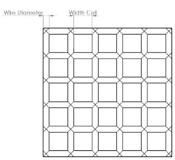
The Reynolds number and the mesh factor comes determined by the mesh that will be used for the screen, while the porosity needs to be calculated with the wire diameter and the weave density; it also depends on geometric factors, in this case, we will use a square one, so we calculate the weave density as:

(30)

𝜌 = 1 𝑤⁄ 𝑚

With 𝑤𝑚 the width of one square cell. With the weave density calculated now we can calculate the

porosity,

𝛽𝑠 = (1 − 𝑑𝑤𝜌𝑚)2

Figure 6 Mesh example

The compliment of the porosity is the screen solidity, which is the ratio between the cross-section area occupied by the metal sheet and the total cross-section area,

𝜎_𝑠 = 1 − 𝛽_𝑠

Mesh factors are given by Idel’chik [6] and these are: 1.0 for new metal wire, 1.3 for average circular metal wire and 2.1 for silk thread.

Once these parameters are calculated, we can determine the coefficient loss by the next expression, 𝐾_𝑚 = 𝐾_{𝑚𝑒𝑠ℎ}𝐾_𝑅𝑛𝜎_𝑠+ (𝜎𝑠

𝛽_𝑠)

2

Where 𝐾𝑅𝑛 is: for 0 ≤ 𝑅𝑒𝑤 < 400

𝐾𝑅𝑛= [0.785 (1 −

𝑅_𝑒𝑤

354) + 1.01] And, for 𝑅𝑒𝑤 > 400,

(31)

Honeycombs

As stated in the previous section, the design parameters are: length (𝐿ℎ), cell hydraulic diameter (𝐷ℎ)

and the porosity (𝛽ℎ).

The length usually comes determined by the fabricant of the honeycomb mesh; but if it’s possible to choose it, the length needs to be long enough to rendered parallel the flow, eliminating the transverse turbulence but not long enough to generate a boundary layer capable of disrupting the flow (turbulent) and introducing new turbulence.

The porosity of the honeycomb mesh is calculated the same way as the screen with the difference that now the wire diameter is replaced with the thickness of the cell (𝑠ℎ𝑜𝑛𝑒𝑦) and the width of the mesh with

the cell size (𝑑ℎ𝑜𝑛𝑒𝑦); knowing that the density is 𝜌 = 1 𝑑 ℎ𝑜𝑛𝑒𝑦

⁄ , introducing it into the equation for the porosity, this one now is,

𝛽_𝑠 = (1 − 𝑠ℎ𝑜𝑛𝑒𝑦 _𝑑

ℎ𝑜𝑛𝑒𝑦

⁄ )

2

The hydraulic diameter is a term used when handling flow in non-circular tubes and channels; with this term, one can calculate many things in the same way as for a round tube as for example, the Reynolds number. This can be calculated with the generic equation:

𝐷_ℎ = 4𝐴 𝑃 Where:

𝐴 = 𝑐𝑟𝑜𝑠𝑠 − 𝑠𝑒𝑐𝑡𝑖𝑜𝑛 𝑎𝑟𝑒𝑎 𝑜𝑓 𝑡ℎ𝑒 𝑓𝑙𝑜𝑤 𝑃 = 𝑤𝑒𝑡𝑡𝑒𝑑 𝑝𝑒𝑟𝑖𝑚𝑒𝑡𝑒𝑟 𝑜𝑓 𝑡ℎ𝑒 𝑐𝑟𝑜𝑠𝑠 − 𝑠𝑒𝑐𝑡𝑖𝑜𝑛

In our case, being the shape a regular hexagon, because we are talking about a honeycomb, we can calculate the perimeter and area with the equations for this shape; being a regular hexagon, all the angles are 120°. And the center angle, which is the angle formed between the center of the hexagon and two lines that join this one with two consecutive vertex is,

𝛼 = 360° 𝑁 =

360°

(32)

Figure 7 Hexagon example

In this case, we have the cell size, which is two times the apothem, and the tangent of the half of the center angle, we can calculate the length of the side of the honeycomb.

𝑎𝑝 = 𝑑ℎ𝑜𝑛𝑒𝑦 2 𝑎𝑝 = 𝑑ℎ𝑜𝑛𝑒𝑦 2 = 𝑙_{ℎ𝑜𝑛𝑒𝑦} 2 tan(𝛼 2) => 𝑙_{ℎ𝑜𝑛𝑒𝑦} = 𝑑_{ℎ𝑜𝑛𝑒𝑦} tan(𝛼 2) = 𝑑ℎ𝑜𝑛𝑒𝑦 tan(30°)

Once we know the length of the side of the hexagon we can calculate both the perimeter and the area of the hexagon. The perimeter is the sum of the length of the six sides of the hexagon; in this case is a regular one so the perimeter is,

𝑝𝑒𝑟𝑖𝑚𝑒𝑡𝑒𝑟_{ℎ𝑜𝑛𝑒𝑦} = 6 ∗ 𝑙_{ℎ𝑜𝑛𝑒𝑦}

The area is calculated as half the product between the perimeter and the apothem. Because the perimeter is six times the length of the side, the area is,

𝐴𝑟𝑒𝑎_{ℎ𝑜𝑛𝑒𝑦} = 3 ∗ 𝑙_{ℎ𝑜𝑛𝑒𝑦}∗ 𝐴𝑝 𝐴𝑟𝑒𝑎ℎ𝑜𝑛𝑒𝑦= 3 ∗ 𝑙ℎ𝑜𝑛𝑒𝑦∗ 𝑙ℎ𝑜𝑛𝑒𝑦 2 tan (𝛼 2) 𝐴𝑟𝑒𝑎ℎ𝑜𝑛𝑒𝑦= 3 ∗ 𝑙ℎ𝑜𝑛𝑒𝑦2 2 tan (𝛼 2)