ALMA MATER STUDIORUM - UNIVERSITÀ DI BOLOGNA
CAMPUS DI CESENA
SCUOLA DI INGEGNERIA E ARCHITETTURA
CORSO DI LAUREA MAGISTRALE IN INGEGNERIA BIOMEDICA
TITOLO DELLA TESI
UNCERTAINTIES ANALYSIS OF
DIGITAL VOLUME CORRELATION MEASUREMENTS FOR
SYNCHROTRON-BASED TOMOGRAPHIC IMAGES OF BONE
Tesi in
Meccanica Dei Tessuti Biologici Lm
Relatore
Prof. Luca Cristofolini
Correlatore
Dr. Enrico Dall’Ara
Presentata da
Comini Federica
i
Acknowledgements
I would like to acknowledge my supervisor Prof. Luca Cristofolini for the opportunity and for his advice during the writing of this thesis. I would like also to thank Dr. Enrico Dall’Ara of the University of Sheffield for his constantly help, guidance and support. His knowledge and motivation taught me how to deal with the difficulties that may be encountered during the research work.
My sincere thanks also go to the University of Sheffield members, in particular, to the experts who gave me technical support for this research thesis: Dr. Will Furnass, Mr. Will Griffiths and Mr. Ben Hughes. I’m grateful to Dr. Mario Giorgi for helping me with the DVC analysis and to Dr. Pinaki Bhattacharya for sharing his data.
ii
Abstract
The evaluation of the heterogeneity of the strain inside the bone tissue is important for assessing the effect of bone pathologies and interventions and for validating computational models. Digital Volume Correlation (DVC) has been proved to be a powerful technique to measure internal displacement and strain field in bone. Recent studies have shown that the synchrotron radiation micro-computed tomography (SR-microCT) can improve the accuracy of the DVC but only zero-strain or virtually-moved test have been used to quantify the DVC uncertainties, leading to potential underestimation of the measurement errors. In this study, for the first time, the uncertainties of a global DVC approach have been evaluated on virtually deformed repeated images to account for the image noise and for a known applied deformation. Virtually-deformed tests have been carried out from repeated SR-microCT scan of bovine cortical bone specimens with a nominal resolution of 1.6 μm. Different levels and directions of deformation have been simulated and the strain fields have been computed with the Sheffield Image Registration Toolkit (ShIRT) combined with a finite element software package. The amount and distribution of the errors for each component of strain have been evaluated. The analysis showed that systematic and random errors of the normal strain components along the deformation direction were higher than the errors in the components at zero strain. The estimated systematic error, for 1% of nominal compression, was approximately 10% of the nominal applied deformation, while the random errors ranged between 10 and 15%. Higher errors have been localized in the boundary of the volumes of interest, perpendicular to the deformation direction. When 120 µm of the edge were removed from the analysis, the systematic and random errors have been reduced to approximately 6% and 7% of the applied deformation. In conclusion, when this technique is used, all the sources of errors need to be considered and, for each application, an optimization of the registration and post-processing parameters of the DVC analyses is suggested. To complete the evaluation of the DVC uncertainties, future studies should use the method presented here but applying a realistic heterogeneous strain field.
1
Contents
1. Introduction 3
1.1. Bone 5
1.1.1. Bone composition 5
1.1.2. Bone microscopic and macroscopic structure 6
1.2. Morphological analysis 10
1.2.1. Micro Computed Tomography (Micro-CT) 10
1.2.2. Synchrotron radiation micro-CT (SR micro-CT) 12
1.3. Strain measurements in bone 14
1.4. DVC applications 18
1.5. DVC accuracy and precision 19
1.6. Study aims 23
2. Materials and methods 24
2.1 Specimens and SR micro-CT 24
2.2 Image processing 25 2.2.1 Uniaxial deformations 26 2.2.2 Composed deformations 28 2.3 DVC protocol 28 2.4 Uncertainties analysis 32 3. Results 37 3.1 Frequency plot 37 3.2 Systematic errors 45 3.3 Random errors 48 3.4 Scalar indicators 51
3.5 Systematic and random errors for different nodal spacing 53
3.6 Spatial distribution of the errors 55
3.7 Effect of the edge 59
3.8 Composed deformation 66
4. Discussion 68
4.1 Limitations and potentials future works 77
5. Conclusion 78
2
3
1. Introduction
Musculoskeletal pathologies, such as osteoporosis, osteoarthritis and bone metastases are related to the bone fracture risk. One of the main aims of bone research is to assess the risks of fracture in bone and to prevent their occurrence. The bone is a complex heterogeneous and anisotropic material and it is a result of a structural optimization, especially from the mechanical point of view (Cristofolini, 2015). Bone structure can resist complex physiological loading and regulate its mechanical resistance through remodelling.
The information of the full field strain in the bone at the organ and tissue level is important from the clinical point of view for many reasons. First, it is known that mechanical and physiological environment have a strong influence in bone remodelling. In fact, changes in bone tissue structure, shape and composition are driven by the amount and distribution of strain (Lanyon et al., 1996; Petrtyl and Danesova, 1999; Rosa et al., 2015). Moreover, the knowledge of internal strain can be useful to understanding the potential pathogenesis of bone fractures (Hussein et al. 2012; Christen et al.,2012). Furthermore, the evaluation of the bone strain and fractures mechanism at the local level may help to generate strategies for prevention and treatment (Cowen, 2001; Danesi et al., 2016).
The finite element method (FEM) is a computational technique which can be used to solve the biomedical engineering problems. In recent years,in order to estimate the bone fracture risk, these computational models have been used to predict the bone mechanical properties (Bessho et al., 2007; Falcinelli et al., 2016). However, FEM verification and validation are fundamental as their output can be considered to have any clinical value (Viceconti, 2005). Validation of these computational models is usually performed only on apparent properties of the bone (e.g. stiffness and strength) which are much easier to test than the local ones.
Experimental measurements of local bone strains are needed for assessing the effect of pathologies and interventions and for validating computational models. Different techniques, such as strain gauges or digital image correlation (DIC), have been used to evaluate the strains on bone at organ- and tissue-level (Grassi and Isaksson, 2015). However, these methods offer measures only on the external surface. Digital
4
Volume Correlation (DVC) is a technique introduced by Bay and colleagues in the 1999 to measure displacement and strain inside the bone (Bay et al., 1999). They described this method as the three-dimensional extension of the DIC. To date, the implementation of the DVC is not unique and different algorithms have been proposed (Roberts et al., 2014). High-resolution X-ray Computed Tomography, or micro-CT, images of the bone are typically used in the correlation algorithm. These types of images allow the internal microarchitecture to be visualized, with resolutions at micrometre level. The DVC is based on tracking the displacement of the microstructural features within image volumes from two scans of the same bone sample, in both unloaded and loaded state (Grassi and Isaksson, 2015). The strain measurements are then computed from the displacements field by differentiation.
Many applications of the DVC to measure displacement and strain inside bone structures and biomaterials are reported in the literature so far (Bay et al., 1999; Liu and Morgan, 2007; Bay et al., 2008; Hussein et al., 2012; Madi et al., 2013; Gillard et al., 2014; Danesi et al., 2016; Palanca et al., 2016; Zhu et al., 2016; Tozzi et al., 2017). Recently, some studies have qualitatively compared the full field displacement and strain measurements of the DVC to same quantities predicted by the FE models generated for the same bones (Zauel et al., 2006; Jackman et al., 2016; Chen et al., 2017; Costa et al., 2017). Still low accuracy and precision is achieved for strain measures at the level of a single bone structural unit. For this reason, a direct comparison between measurements from the FE models to DVCs could be performed only for the displacement field (Chen et al., 2017; Costa et al.,2017). However, as the bone fails after a certain level of strain, the prediction of local strain becomes fundamental and an accurate DVC method is needed to evaluate the heterogeneity of the strain inside the bone, even at a local level. Two recent studies reported that high-resolution images, based on synchrotron radiation (SR micro-CT), can improve the accuracy and precision of the DVC displacement and strain measurements (Christen et al.,2012; Palanca et al., 2017). However, the estimation of DVC precision in strain measurements is usually based only on a specific case of zero-strain condition and it remains to be investigated what DVC precision and accuracy can be obtained under load.
5
1.1. Bone
The bone tissue is the main constituent of the skeleton and it differs from other connective tissues for mineralization of the extracellular matrix. Two types of bone tissue can be distinguished: cortical and trabecular bone which differ mainly in terms of development, density, architecture, function, proximity to the bone marrow, blood supply, rapidity of turnover time and fractures (Cowin, 2001). The following paragraphs will provide a brief description of the bone composition and structure at both microscopic and macroscopic level.
1.1.1. Bone composition
The bone is constituted for 65% by inorganic components (minerals) and for 35% by organic matrix, cells, and water. The mineral part is mainly impure hydroxyapatite, Ca10(PO4)6(OH)2, containing constituents such as carbonate, citrate, magnesium, fluoride, and strontium. The bone mineral is in the form of small crystals in the shape of needles, plates, and rods located within and between collagen fibres. The organic matrix consists of 90% collagen and about 10% of various noncollagenous proteins. Bone cells are fundamental for the modelling and remodelling of the extracellular matrix as well as the calcium homeostasis. The cells in the bone belong to three families: osteoblasts, osteoclasts and osteocytes. Osteoblasts are bone-forming cells that synthesize and secrete unmineralized bone matrix, participate in the calcification and resorption of bone, and regulate the flux of calcium and phosphate across the bone. Osteoclasts are multinucleated giant cells and their function is to resorb both the mineral and organic component of the bone. Lastly, osteocytes are the most abundant cell type in mature bone and they are involved in the homeostatic, morphogenetic, and restructuring processes of bone mass. Basically, the osteocytes play a key role in the biological and mechanical regulation of bones (Cowin, 2001).
Both the mineral and organic parts of bone have important mechanical functions. The mineral part gives stiffness, which is fundamental for the support function of the bones as well as the transmission of muscular forces. On the other hand, the collagen provides tenacity to the bone, necessary to protects the soft tissues of the cranial, thoracic and pelvic cavities.
6
1.1.2. Bone microscopic and macroscopic structure
Bone tissue at the microscopic level is classified into two types: woven and lamellar (Cowin, 2001). The first one consists in a matrix of interwoven coarse collagen fibres and the osteocytes have a random distribution. Lamellar bone is made up of unit layers (lamellae), each lamella is approximately 3 to 7µm thick and contains fine fibres that run in approximately the same direction. The woven bone is less organized and shorter-lived than lamellar bone. In the developing embryo the bone is the woven type and then resorbed and replaced by lamellar bone.
The lamellae of the cortical bone appear in different patterns to form three structures: osteon, circumferential lamellae, and interstitial lamellae (Figure 1). In the osteon, or Haversian system, the lamellae are willing in circular rings surrounding a longitudinally vascular channel, the Haversian canal. Within this canal run blood, lymphatics vessels and nerves. Haversian canals are interconnected by transverse canals, also called the Volkmann canals. The circumferential lamellae consist on several layers of lamellae extending around the circumference of the bone shaft. The interstitial lamellae are angular fragments of bone composed of the remnants of past generations of osteons or circumferential lamellae and they fill the gaps between Haversian systems.
7
Throughout woven and lamellar bone there are the lacunae, small cavities, in which osteocytes are entrapped. Radiating from the lacunae are tiny canals, or canaliculi, into which the long cytoplasmic processes of the osteocytes extend. These canals and the Haversian and Volkmann channels, form a 3D network that provides supply to the cells. The outer surface of most bone is covered by the periosteum which is a sheet of fibrous connective tissue and an inner cellular or cambium layer of undifferentiated cells. The periosteum has the potential to form bone during growth and fracture healing. The marrow cavity of bones is lined with a thin cellular layer called the endosteum which is a membrane of bone surface cells.
At the macroscopic level, the bone can be classified as cortical (or compact) or trabecular (or spongy). The distribution of cortical and trabecular bone varies significantly between different bones. Approximately 80% of the skeletal mass in the adult human skeleton is cortical bone and the remaining 20% is trabecular bone (Cowin, 2001). These types of bone tissue can be easily distinguished by their degree of porosity and density (Figure 2). The cortical bone is very dense and with a low porosity (5-10%), while the trabecular bone appears as a sponge with a porosity that varies between 45-95%.
Figure 2: Cross-section of human femoral head showing trabecular and cortical bone. Source from http://medcell.med.yale.edu/systems_cell_biology/bone_lab.php
In the trabecular bone, the structural unit is the trabecular packet (Figure 3). In general, it lacks osteonal structure and consists of a mosaic of angular segments of parallel sheets of lamellae preferentially aligned with the orientation of the trabeculae.
8
The ideal trabecular packet is shaped like a shallow crescent with a radius of 600 µm and is about 50 µm thick and 1 mm long. The trabecular packets are hold together with cement lines, layer of mineralized matrix deficient in collagen fibres. Trabecular bone is not populated by the Haversian or Volkmann channels and the osteocytes are feed directly from the marrow.
Figure 3: Scanning electron micrograph (SEM) of trabecular bone of the human shin. Source fromhttps://fineartamerica.com/featured/7-sem-of-human-shin-bone-science-source.html.
Cortical bone cortical is a dense, solid mass with only microscopic channels and the main structural unit of cortical bone is the osteon or Haversian system (Figure 4). Osteons form approximately two thirds of the cortical bone volume; the remaining one third consist of interstitial and circumferential lamellae. A typical osteon is a cylinder about 200 or 250 µm in diameter and it is made up of 20 to 30 concentric lamellae. Each osteon is surrounding by a cement line, a 1- to 2-µm-thick. The Haversian canals are interconnected by the transverse Volkmann’s canals within run blood vessels, lymphatics and nerves.
9
Figure 4: Cross-section of human compact bone shows the Haversian system (or osteon), the central canal and the lacunae. Source from https://mesa-anatomy.weebly.com/supportive-connective-tissue.html
Plexiform or laminar bone is a type of bone tissue in cortical bone of the long bones in large rapidly growing mammals such as cows and pigs and less frequently in the bones of primates, including humans (Figure 5). Plexiform bone consists of alternating layers of parallel-fibred bone and lamellae forming a brick-like structure. Each "brick" bone is about 125 μm across. This type bone also contains cores of non-lamellar bone and blood vessels surrounded by intercalating lamella bone. For instance, a bovine cortical bone may present microstructures with haversian bone, plexiform bone, or both together depending on the position considered. The two microstructures of haversian and plexiform bone have different mechanical properties (Kim et al., 2007). The fatigue strength of plexiform bone is higher than that of haversian bone.
Figure 5: Optical micrographs of: (a) haversian and (b) plexiform bones of posterior and anterior of bovine femoral compact bones (Kim et al., 2007).
10
1.2. Morphological analysis
Micro-computed tomography (micro-CT) has become a standard tool for the evaluation of bone morphology and microstructure (Bouxsein et al., 2010). This type of imaging technique allows the three-dimensional (3D) nature of the bone structure to be visualised with high resolutions and in a non-destructive way. Different micro-CT systems with different hardware and scanning modalities are available and can achieve different spatial resolution (signal-to-noise ratio). The synchrotron radiation micro-CT (SR micro-CT) technique has also been used to investigate bone micro-architecture. The choice of spatial resolution is fundamental to observe in the image the features of a given structure. In standard laboratory micro-CT systems trabecular bone is generally imaged with voxel size between 5 μm and 20 μm, corresponding to fields of view of several centimeters but to visualize imaging lacunae and canaliculi in cortical bone, spatial resolutions at the micrometer or the nanometer scale is required, achievable with Synchrotron technology or nano-CT systems (Peyrin et al. 2014, Dong et al., 2014).
1.2.1. Micro Computed Tomography (Micro-CT)
Micro-CT systems use similar technology as clinical CT but allow to achieve better resolution. It is a powerful imaging technique for the characterization of different types of materials from the microstructural point of view. Similarly to clinical CT, micro-CT techniques is based on the interaction of the X-rays with the sample. A tomographic system, without considering the computer for the acquisition and reconstruction of images, is mainly composed by three elements: the X-ray source, the sample rotation system and the detector (Figure 6).
In most standard desktop micro-CT system, the sample is placed between the source and the detector on a rotary table. The angle of rotation of the sample and the rotation step between the individual projection images are parameters that can be chosen in most scanners. The detector has the function of measuring the intensity of the transmitted X-rays after they have interacted with the sample. Currently, there is a wide range of detector systems with properties that are very different from each other. At each rotation step the detector acquires a two-dimensional image, called projections, which are used to reconstruct a three-dimensional image of the same object.
11
Figure 6: Configuration of a micro-CT scanner with a sample rotating within a stationary X-ray
system
Typically, micro-CT systems operate in the range of 20 to 100 kVp, and the attenuation of the X-ray photons as they pass through material can be caused by either absorption or scattering depending on their energy (Bouxsein et al., 2010). The interaction of lower energy X-rays (less than 50 keV) is dominated by the photoelectric effect and depends on the atomic number of the materials. The photoelectric effect occurs when a photon interacts with an electron of the innermost orbits of the material’s atom. In the collision, the photon is absorbed with the consequent emission of an electron (called photoelectron). At low energies, only small objects can be observed, otherwise noise becomes too large to allow quantitative analysis. The interaction of higher-energy X-rays (higher than 90 keV) is dominated by Compton scattering, where the attenuation is approximately proportional to the density of the material. The Compton effect consists in the inelastic collision of a photon with an electron belonging to an external orbital of the material’s atom. In the interaction, the photon is diffused in a different direction and with a different wavelength, while the electron is put in motion with a certain kinetic energy. In the medium range of X-ray energy (from 50 to 90 keV), both the photoelectric effect and Compton scattering contribute to attenuation.
After acquiring the X-ray projection images, the computerised reconstruction of the 3D stack of images from the projection images is performed. The image reconstruction usually includes a beam hardening compensation. This artefact resulting from the fact that the X-ray tubes used in the µCT systems do not produce X-rays of a single energy, but a spectrum of energies. A voxel is defined as the discrete unit of the
12
scan volume that is the result of the tomographic reconstruction. Typically, voxels from micro-CT images have all three dimensions equal and therefore are described as isotropic voxels. The resolution of the image is defined as the smallest feature that can be resolved in the image. Hence, the resolution and voxel size are not equivalent, and their relationship depends on several factors (i.e., mean absorption of sample, detector noise, reconstruction algorithm, X-ray focal spot size and shape, detector aperture, and scanner geometry) (Bouxsein et al., 2010). Small voxel size usually leads to high scan resolution; however, this requires longer acquisition times because more sample’s projections need to be collected and processed. Therefore, a best compromise between the minimum resolution acceptable and the scan time should be find.
1.2.2. Synchrotron radiation micro-CT (SR micro-CT)
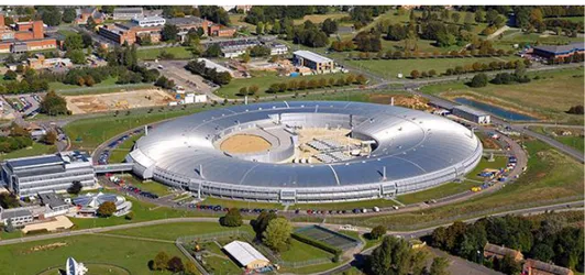
Synchrotron radiation or synchrotron light is an electromagnetic radiation generated by charged particles, usually electrons, moved at very high speeds in a large ring (in the order of kilometres). In the synchrotron facilities an electron gun produces electrons and a linear accelerator (LINAC) accelerates them into the booster ring (Figure 7). The electrons move at an increased rate until almost at the speed of light and system of deflecting magnets curves the path of electrons, forcing them to remain on a circular trajectory. When electrons change their direction, they emit a very high energy radiation. The flux and brilliance of the emitted radiations are increased, and the wavelength band reduce on the X-ray region. At last, the filtered X-rays are addressed in the experimental stations, located at the end of the beamline.
Figure 7: Diamond Light Source, UK. Source from:
13
Using synchrotron sources provides several advantages to the micro-CT compared to the conventional X-rays tubes, especially to achieve images with spatial resolution below the micrometer (Figure 8). First, synchrotron sources offer a photon flux several orders of magnitude higher that both limit the scan times and increase the signal to noise ratio. Moreover, with a synchrotron source it is possible to obtain a monochromatic X-rays beam, that is important to limit the image artifacts such as beam-hardening, which is often a serious limitation for analysis conducted with laboratory X-rays systems that employ a polychromatic beam.
During the past decade, SR micro-CT has been used for the assessment of structure and mineralization in human or animal trabecular bone (Peyrin et al., 2014). Recently, its application on cortical bone allowed to explore the 3D osteocyte lacunar morphometric properties and distributions in human femoral bone with nominal voxel size of 1.4 μm (Dong et al., 2014). Consequently, SR micro-CT offers extremely high-resolution imaging of microarchitecture and mineral density in excised bone specimens. Nevertheless, the main disadvantages of this technique are its limited availability of the access to a synchrotron source as well as the costs (Bouxseis et al., 2010). Moreover, technical expertise needed to set properly the scan parameters to avoid damaging the sample due to the radiations.
14
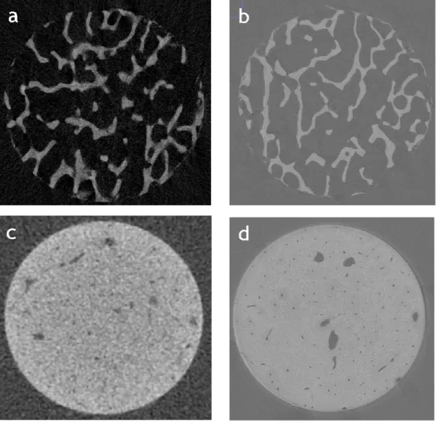
Figure 8: Trabecular (a) and cortical (c) bone scanned with laboratory micro-computed tomography (μCT) at 10 μm voxel size (Dall’Ara et al., 2014). Trabecular (b) and cortical (d) bone scanned with synchrotron light μCT (SRμCT) at 1.6 μm voxel size (Palanca et al., 2017). The figures show the difference in terms of resolution between the μCT and SRμCT images. Indeed, in the cortical bone image scanned with SRμCT (d) it is possible to identify a greater number of features (i.e. osteocyte lacunar and canaliculi) compared to the same tissue image scanned with μCT.
1.3. Strain measurements in bone
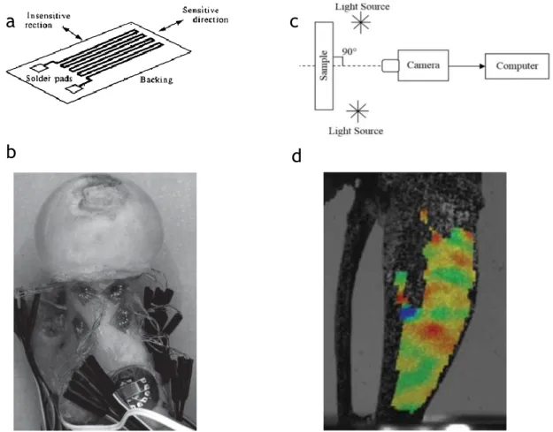
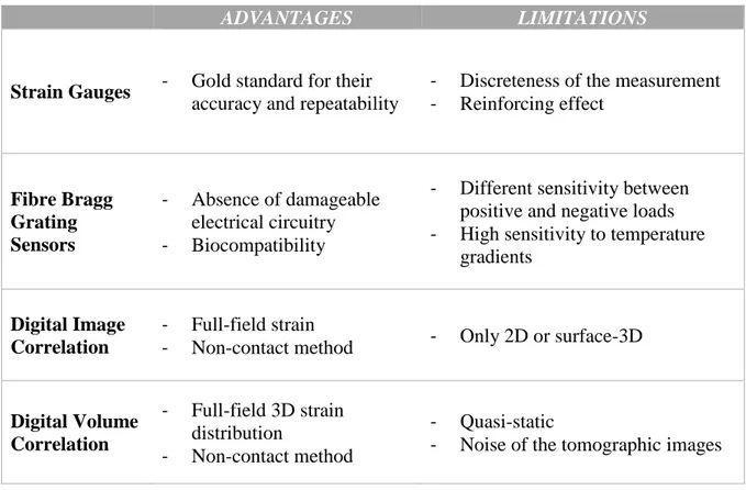
To date, some methods have been used to measure the strains on bone at organ- and tissue-level (Grassi and Isaksson, 2015) (Table1). Strain gauges (SGs) are the first to be used in bone biomechanics for strain measurements and they are still considered the gold standard for their accuracy and high frequency response (Cordey and Gautier, 1999; Cristofolini et al., 2009) (Figure 9). Nevertheless, SGs have a non-negligible
15
stiffness that can affect the strain measurement. Moreover, SGs application is limited mainly for the discreteness of measurements.
Figure 9: a: A schematic representation of a strain gauge. b: Strain gauges are bonded in the different regions of the proximal femur used for point-wise measurement of strain on the bone surface (Cristofolini et al., 2010). c: A schematic diagram of the experimental set-up for 2D-DIC system (Khoo et al., 2016). d: Mouse tibia surface strain measured with the digital image correlation technique (Pereira et al., 2015).
Fibre Bragg grating sensors (FBGS) can be a possible alternative to the strain gauges for measures at the interface between two materials (Fresvig et al., 2008). This is possible thanks to the absence of damageable electrical circuitry. However, FBGS application in bone biomechanics is still restricted for their lower accuracy and precision compared to strain gauges. Digital Image Correlation (DIC) is a non-contact method, which allows to measure strain over a large portion of the surface of the specimen (Palanca et al., 2016) (Figure 9). With this technique, one digital image is mapped onto another and the transformation field is determined by maximizing a correlation coefficient. Hence, the “reinforcement effect” does not occur when this
a
c
16
technique is used. In order to make the area of the specimen surface univocally identifiable, a speckle pattern is usually added. The spatial resolution of the DIC depends on the quality of the acquired images, on the applied speckle, and on the parameters of the correlation algorithm that should be optimized for every specific application.
However, all the methods mentioned above can measure strain only on the external surface of the bone specimens. The Digital Volume Correlation is the extension of the DIC to the third spatial dimension (Bay et al., 1999). DVC application on bone is recent and, to date known, it is the only method that can measure the internal strain field. Two volume images, one undeformed and one deformed, are used as the input of the DVC algorithm. The power of this technique is particularly due to the high resolution computed tomography (micro-CT or SR micro-CT) that allows slice images and 3D volumes of the internal microarchitecture to be generated, with resolutions of micrometre level. Therefore, the DVC is able to correlate the natural features in the 3D images, without the need of adding speckles. In the local DVC approach, the 3D volume is divided in to several sub-volumes which are registered and represented as a discrete function: 𝑓(𝑥, 𝑦, 𝑧) and 𝑔(𝑥 + 𝑖, 𝑦 + 𝑗, 𝑧 + 𝑘) for the offset (𝑖, 𝑗, 𝑘) in the x, y and z direction respectively (Figure 10). The displacement measurement step involves minimization of an objective function that quantifies the match between original and deformed subvolumes with respect to a set of affine transformation parameters (Bay, 2008). Finally, strains are estimated at all the measurement locations from the displacement vector field.
In order to recognize features in the two images and estimate the displacements and strain 3D fields, different DVC approaches with a number of computational strategies have been developed so far (Roberts et al., 2014; Palanca et al., 2015). The principal limit of the DVC is that the measurements are affected by the noise of the tomographic images (Dall’Ara et al. 2014). Since his introduction, a number of studies were performed to estimate the DVC accuracy and precision. Some examples are given in the next paragraph to show how the displacement and strain measurement errors are evaluated.
17
Figure 10: In the DVC algorithm, the image volumes are divided into sub-volumes represented with the functions f(x, y, z) and g(x+i, y+j, z+k) in the unloaded and deformed images respectively. An average displacement is computed for each subvolumes by finding the offset (i,j,k) that maximises a cross-correlation function (Gillard et al., 2014).
ADVANTAGES LIMITATIONS
Strain Gauges - Gold standard for their
accuracy and repeatability
- Discreteness of the measurement - Reinforcing effect Fibre Bragg Grating Sensors - Absence of damageable electrical circuitry - Biocompatibility
- Different sensitivity between positive and negative loads - High sensitivity to temperature
gradients
Digital Image Correlation
- Full-field strain
- Non-contact method - Only 2D or surface-3D
Digital Volume Correlation - Full-field 3D strain distribution - Non-contact method - Quasi-static
- Noise of the tomographic images
18
1.4. DVC applications
The DVC was introduced for the first time to determine the 3D displacement and strain fields in trabecular bone (Bay et al., 1999). Since then, DVC has seen many applications as no other methods can give measurements of displacement and strain within samples. This technique is therefore ideal to investigate the internal strain distribution and the local damage inside bone, biomaterials or at the interface between them (Bay et al., 1999; Liu and Morgan, 2007; Hussein et al., 2012; Madi et al., 2013; Gillard et al., 2014; Danesi et al., 2016; Zhu et al., 2016). Consequently, the DVC can be very useful to address clinical and preclinical problems as well as validate Finite Element models (Zauel et al., 2006; Jackman et al., 2016 Chen et al., 2017; Costa et al.,2017).
To give some example, in a recent study, in order to understand the failure mechanism in prophylactically augmented vertebrae under compression, a DVC method was used for investigating the full-field strain distribution, from the elastic regime until failure (Danesi et al., 2016) (Figure 11).
Figure 11: On the left-side: Strain map of murine cortical bone for the second load step after the initiation of the first microcracks. Transverse plane with the osteocyte lacunae (yellow), the microcrack (green) and the canals (red) (Christen et al., 2012). On the right-side: Internal strain distribution for 5% of compression in augmented vertebrae. The axial component of strain (in microstrain) is shown for the specimen over the sagittal slice (Danesi et al., 2016).
In a different study, the local strains distribution in murine femora have been measured during the initiation and propagation of microcracks using a SR-CT -based DVC (Christen et al., 2012) (Figure 11). This approach allowed to achieve spatial resolution of both displacement and strain approximately of 10 µm. Recently, a DVC
19
method has been used to validate a micro Finite Element models to predict the local displacement across the whole vertebral body under different degree of compression (Costa et al., 2017). The results of that study showed also a qualitative agreement between the strain distribution measured with DVC and predicted by the micro-FE models from all the specimens. However, a direct quantitative strain comparison could not be performed because, for a reasonable precision of the DVC, the nodal spacing should be 50 times higher than the element size of the micro-FE elements.
1.5. DVC accuracy and precision
Accuracy and precision of displacement and strain measurements obtained using DVC depend of several factors such as the quality of the volume images, the parameters in the correlation algorithm and the type of bone (Liu and Morgan, 2007; Roberts et al., 2014; Dall’Ara et al., 2017) (Table 2). To date, there is no gold standard for the assessment of accuracy and precision of the DVC due to the lack of other accurate technique able to measure internal displacements and strains (Palanca et al., 2015). The repeated-scans test in zero-strain condition is the most commonly adopted method for uncertainties measurement (Bay et al., 1999; Liu and Morgan, 2007; Dall’Ara et al., 2014; Palanca et al., 2015; Palanca et al., 2016). This type of test allows to evaluate the accuracy and precision including the effect due to the intrinsic noise of the micro-CT images (Dall’Ara et al., 2014). Another procedure to measure errors is the simulated-displacement test (or virtually-moved test) which is constructed from a single scan of a given specimen by translating the image volume by a uniform amount in each coordinate direction (Liu and Morgan, 2007; Dall’Ara et al., 2014; Palanca et al., 2015). This test is carried out usually to obtain a controlled displacement with a zero-strain field. However, in the simulated-displacement test the uncertainties are underestimated because the image noise is traced as a feature of the image. For this reason, in the repeated-scans test the error are generally larger than the ones compute for the simulated displacement (Dall’Ara et al., 2014).
Initially, the precision of the DVC in trabecular bone sample was measured by Bay with a repeated-scan test (Bay et al.,1999). Using an X-ray tomography with a resolution of 35 µm, in that study the strain measurement precision obtained was approximately of 300 µstrain. Afterwards, in another study the DVC has been applied at
20
different trabecular structures to measure displacements and strains (Liu and Morgan, 2007). Investigating several bone samples from different species and anatomical sites, that study showed how the accuracy and precision of DVC depend on the sample microstructure as well as on the computational approach. The maximum likelihood estimation (MLE) method used in that study achieve better results and, across all bone types tested, the displacement and strain precision errors ranged 1.86-3.39 µm and 345-794 µɛ, respectively. In particular, strain precision and accuracy were highest for specimens with lower volume fraction (BV/TV) and trabecular number (Tb.N), and higher trabecular spacing (Tb.Sp) and structural model index (SMI).
Reference
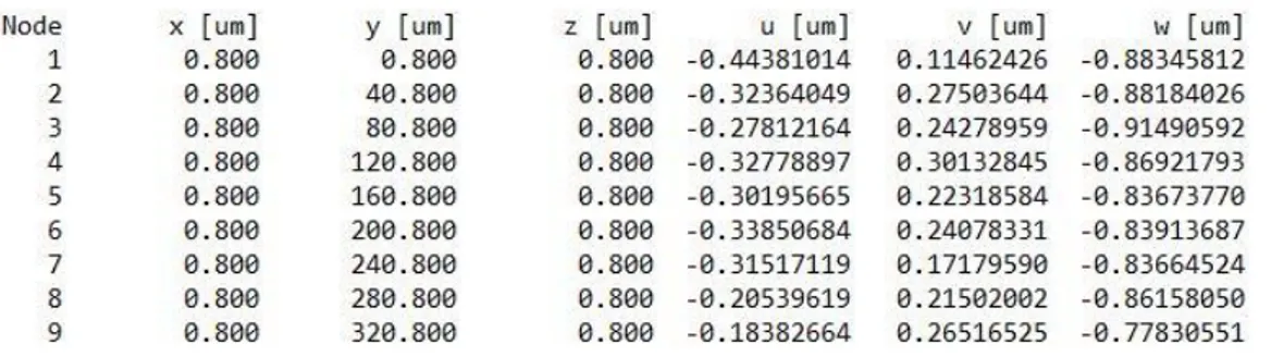
Imaging Bone type voxel size (µm) Sub-volum e (voxel) Measured displacement * (µm) Measured strain* (µstrain) Accurac y Precision Accurac y Precision Bay et al.,
1999 µCT Trabecular 35 61 N.A. 1.23 N.A. 302-288 Liu and Morgan, 2007 µCT Trabecular 36 40 -0.14 1.86-3.39 345-794 N.A. Hussein et al., 2012 µCT vertebral bodies 37 N.A. 21.46 41.44 740 630 Christen et
al., 2012 SR-µCT Cortical 0.74 25 0.0004 0.13 N.A.
11000-13000 Dall'Ara et al., 2014; Palanca et al., 2015 µCT Trabecular Cortical 10 15** N.A. 2270 2781 ⁓ 4000 ⁓ 5000 ⁓ 2400 ⁓ 2600 Palanca et al., 2016 µ CT vertebral bodies 39 16 N.A. 302 ⁓ 300 ⁓ 700 Palanca et al., 2017 SR-µCT Trabecular Cortical 1.6 100** N.A. 64 21 ⁓ 240 ⁓ 55 ⁓ 110 ⁓ 20
Table 2: Overview of the DVC accuracy and precision estimate with different parameters. *Value referred as average of the errors across the different directions.
21
For a more extensive assessment of the accuracy and precision of the DVC to measure the displacement and strain, both cortical and trabecular bone samples have been investigated (Dall’Ara et al. 2014). They found that the main source of error in the output of the DVC was due to the intrinsic noise of the micro-CT images. Moreover, that study showed that the uncertainties decreased as a power low by increasing the nodal spacing (i.e. distance between the nodes of the grid used for displacement and strain calculation), for all bone types. Therefore, a compromise between spatial resolution and measurements errors should be achieved when the DVC method is used. In that study, a nodal spacing of 600-700 µm for cortical and trabecular samples is suggested to discriminate yielded from non -yielded regions with accuracy and precision around 200 µɛ.
A comparative study between three different DVC computational approaches was conducted on cortical and trabecular bone samples (Palanca et al., 2015). Both repeated-scan and virtually-move test were used to quantify the accuracy and precision of the DVC approaches. Beside the different errors obtained from the three methods, it has been confirmed that the accuracy and precision tended to improve for larger sub-volume size (if the local method is used) or nodal spacing (if the global method is used) with an asymptotic trend over 30 voxels for the displacement and 50 voxels for the strains (with a voxel size of 9.96 µm). These parameter values could be used as a trade-off between spatial resolution and errors when the methods are applied to bone tissue.
In the studies mentioned above, it has been shown that with the micro-CT-based DVC uncertainties are too high for strain measurements performed at the bone structural unit level (Liu and Morgan, 2007; Dall’Ara et al., 2014; Roberts et al., 2014). Christen et al. used for the first time the synchrotron radiation-based computed tomography (SR micro-CT) to increase the spatial resolution of the DVC input images (Christen et al., 2012). In that study, a systematic error of the strain not significantly different from zero was achieved, while the precision was approximately 0.012 strains. However, to assess the accuracy and precision only a virtually-moved test was performed, which, as mentioned above, leads to underestimated errors (Dall’Ara et al., 2014). To overcome this problem, in a recent study Palanca et al. performed a zero-strain test on different bone types scanned with a SR micro-CT (Palanca et al., 2017). The uncertainties related to the strain measurements were lower than those obtained with traditional micro-CT images for all bone types with a spatial resolution of the measures around 40 µm to
22
keep uncertainties below 200 microstrain. The greatest improvement was found for cortical bone samples because at that resolution more features were identified in the bone microstructure, helping the correlation algorithm. In order to measure the DVC uncertainties under load, a virtually-compressed and a virtually-compressed-repeated test were performed on cortical bone sample (Palanca et al., 2017- Supplementary material). With the latter method, larger systematic and random errors were obtained due to the effect of the image noise. While this approach is an elegant way of testing the precision of the DVC measurements for under load, its application is limited to the mentioned study and more loading levels and mechanisms need to be explored to fully characterize the outcomes of DVC algorithms applied to SR micro-CT images (Dall’Ara et al., 2017).
23
1.6. Study aims
The Digital Volume Correlation provides internal displacement and strain fields of the bone. Many applications might take advantage from this method as the validation of the computational models. Using micro-CT images, acceptable precision on displacement measurements have been achieved with the DVC. However, for the strain field high uncertainties have been found and a compromise should be accepted between spatial resolution and precision of measurement. Recent studies have shown that the synchrotron radiation micro-CT can reduce the errors of the DVC, especially in the cortical bone. With this approach, adequately low uncertainties in the strain measures can be achieved with spatial resolution around 40 µm. Nevertheless, the accuracy of the DVC approach to measure internal strain of loaded bone structures is still unknown.
The main goal of this work is to develop a method for evaluating the accuracy and precision of SR micro-CT image-based DVC. In this study, different levels and directions of virtually affine deformations are imposed on repeated scans of cortical bone specimens to measure the uncertainties of the DVC.
24
2. Materials and methods
To evaluate the uncertainties of the DVC strain measurements, a new method has been designed in this study. Virtually-deformed tests have been carried out from repeated SR micro-CT scan of cortical bone specimens. Different direction and magnitude of simulated strain have been tested. Afterwards, the full-field strain distributions have been computed with a global DVC protocol.
2.1
Specimens and SR micro-CT
The specimens used in this project to measure the DVC uncertainties were prepared and imaged in a previous work as described in Palanca et al., 2017. Briefly, four 3 mm in diameter and 12 mm in length cortical bone cylinders have been extracted from the diaphysis of a fresh bovine femur (18 months old, killed for alimentary purposes). Tomography scans were performed at the Diamond-Manchester Imaging Beamline l13-2 of the Diamond Light Source, UK. The samples were aligned with the osteons parallel to the rotation axis during data collection. A filtered (950 µm C, 2 mm Al, 20 µm Ni) polychromatic ‘pink’ beam (5–35 keV) of parallel geometry was used with an undulator gap of 5 mm. The propagation distance was approximately 10 mm. Projections were acquired using a pco.edge 5.5 detector (PCO AG, Germany) coupled to a 750 µm-thick CdWO4 scintillator, with visual optics providing 4x total magnification and a field of view of 4.2x3.5 mm. 4001 projection images were collected at equally-spaced angles over 180 degrees of continuous rotation, with an exposure time of 53 ms. With these parameters an effective voxels size of 1.6 µm was obtained. Each specimen was scanned twice under zero-strain conditions and without any repositioning between the two scans (Scan1 and Scan2).
Two cubic volumes of interest (VOIs), with side lengths of 1000 voxels, were cropped from the middle of each reconstructed image. Only one VOI for each couple of scans has been used in this study.
25
Figure 12: 3D representation of the VOIs of the four cortical bone specimens used in this study. Cortical bone scanned with SR-microCT at 1.6 μm voxel size. The side length of each cross section is 1000 voxels. The cube is therefore 1.6 mm in side.
The 3D reconstructions of the four cortical bone specimens are reported in Figure 12. It is possible to note the differences in terms of features’ shape and orientation. The characteristics of the specimens depend on where they have been cored. In particular, they may exhibit a more regular and periodic structure, typical of the plexiform bone (see Specimen 1 and Specimen 2), a more Haversian structure (Specimen 4) or both (see Specimen 3).
2.2
Image processing
In order to evaluate the DVC measurement uncertainties under load, the following procedure has been applied to the cortical bone specimens. The
virtually-1 2
26
deformed-repeated analysis has been performed by registering the original scan (Scan1) with the Scan2 virtually deformed. As explained in the Introduction, this type of test allows to include the effect of the image noise in the DVC uncertainties analysis. Virtual deformations on the repeated scans (Scan 2) were applied using MeVisLab (MeVis Medical Solutions AG, Germany), which includes several modules for the processing and visualization of medical images. In this study, different conditions of load application (single compression and composed deformation), loading directions and load levels have been simulated.
2.2.1 Uniaxial deformations
First, the repeated scans (i.e. Scan 2 of each specimen) have been axially compressed applying 1%, 2% and 3% of deformation. These deformations have been performed separately along X, Y and Z axis, while the other directions were unstrained. Overall, nine deformation conditions have been carried out (Table 3).
Virtual compression Direction X Y Z Lev els 1% 1% 1% 2% 2% 2% 3% 3% 3%
Table 3: Uniaxial compression conditions for each specimen. Three levels of deformation (1%, 2% and 3%) along the three Cartesian directions (X, Y and Z) have been used.
First of all, the module ImageLoad allow to open the image file in different format (in this study DICOM) (Figure 13). Then, the compressions have been applied at the repeated scans using the module AffineTransformation3D. In MeVisLab the three-dimensional affine transformation is performed through a single matrix multiplication:
27
The order for constructing the matrix is shearing, rotation, scaling and translation. To achieve sub-voxel resolution, trilinear interpolation is applied in the input volume using that module. The origin of the coordinate system is in the center of the output volume. Changing the coefficients of this matrix, it is possible to apply various levels of compression in different directions. The coefficients (𝑐) have been computed as:
𝑐 = 1
1 − 𝑑
Where 𝑑 is the deformation imposed. Accordingly, along the directions in which a compression is not desidered, the coefficients have value 1. Lastly, the deformed image can be store in a specific file format with the module ImageSave (in this study DICOM).
Figure 13: Screenshot of MeVisLab script used to apply the single compressions at the repeated scans. In this particular example compression of 1% along Y has been applied.
Coefficients Affine Transformations Deformed Image
28
2.2.2 Composed deformations
A different analysis has been carried out to evaluate the possible effect of simultaneous deformations on the DVC uncertainties. Compressions in the three normal directions (X, Y and Z) within the MeVisLab framework have been performed on the repeated scan of one specimen (Specimen 3). In this case, one level of compression (1%) along three different direction has been simulated simultaneously. The coefficients have been computed as shown in the previous paragraph.
2.3
DVC protocol
In this study a global DVC protocol has been used to compute the strain field: ShIRT-FE (Dall’Ara et al., 2014). It is a combination of an elastic registration software known as Sheffield Image Registration Toolkit (ShIRT) (Barber and Hose, 2005; Barber et al., 2007) and a Finite Element (FE) software package (ANSYS Mechanical APDL v. 14.0, Ansys, Inc., USA). In this DVC approach a homogeneous cubic grid with a certain nodal spacing (NS) is superimposed to the two input images (Scan 1 and Scan 2). Therefore, ShIRT computes the displacements at each node of the grid by solving the registration equations as describe in Barber et al., 2007. Briefly, the procedure consists in finding the displacement functions u(x, y, z), v(x, y, z), and w(x, y,
z) that map the fixed image f(x, y, z) into the moving image m(x’, y’, z’) and, to account
changes in the gray levels, an additional intensity displacement function c(x, y, z) is also included in the equation:
𝒇(𝑥, 𝑦, 𝑧) − 𝒎(𝑥, 𝑦, 𝑧) ≈12(𝑢 (𝜕𝒇𝜕𝑥+𝜕𝒎𝜕𝑥) + 𝑣 (𝜕𝑦𝜕𝒇+𝜕𝒎𝜕𝑦) + 𝑤 (𝜕𝒇𝜕𝑧+𝜕𝒎𝜕𝑧) − 𝑐(𝒇 + 𝒎)) (1)
This equation can be defined for each image voxel. However, there are four unknowns for each equation (u, v, w, c) and the resulting system becomes undetermined. The rank of the problem is reduced by expanding the functions u, v and w in terms of a set of local basis functions. I particular, ShIRT uses tri-linear basis functions centered on the nodes of a superimposed regular cubic grid to interpolate the displacements.
29
𝑣(𝑥, 𝑦, 𝑧) = ∑ 𝑎𝑖 𝑦𝑖𝜑𝑖(𝑥, 𝑦, 𝑧) (3)
𝑤(𝑥, 𝑦, 𝑧) = ∑ 𝑎𝑖 𝑧𝑖𝜑𝑖(𝑥, 𝑦, 𝑧) (4)
In the equations the term 𝜑𝑖(𝑥, 𝑦, 𝑧) is the ith basis function centered at the node with coordinate 𝑥𝑖, 𝑦𝑖, 𝑧𝑖. The coefficients 𝑎𝑗𝑖 of the displacement function are the new unknowns. The Equation (1) can be now written in matrix notation (capital letters represent tensors, low case letters represent vectors) as
𝒇 − 𝒎 = 𝑻𝒂 (5)
where the matrix T is derived from integrals of the image gradients multiplied by the basis functions.
The resolution of the mapping is defined as the spacing between the nodes. If that value is small, then the equation (5) become ill-posed. Therefore, a further constraint is applied by ShIRT to smoothness on the mappings. The result of adding this constraint is to convert the equation (5) to the form:
𝑻𝑻(𝒇 − 𝒎) = (𝑻𝑻𝑻 + 𝜆𝑳𝑻𝑳)𝒂 (6)
where 𝑳 is the Laplacian operator, and λ is a parameter that weights the smoothing. Given a starting value of 𝒂, a correct solution can be computed iteratively. If 𝒂𝑛 is the value of the displacements after n iterations, the updated value is:
𝒂𝑛+1 = 𝒂𝑛 + 𝛥𝒂 (7)
where
𝛥𝒂 = [𝑻𝑻𝑻 + 𝜆𝑳𝑻𝑳]−𝟏(𝑻𝑻(𝒇 − 𝒎(𝒂𝒏)) − 𝜆𝑳𝑻𝑳𝒂𝒏) (8)
To avoid an accumulation of the interpolation errors, at each stage 𝒎(𝒂𝒏) is calculated by applying the current 𝒂 to the original image 𝒎. Iteration stops when the average absolute value of the difference between 𝒂𝑛+1 and 𝒂𝑛 is below 0.1 voxels. After that,
30
the six components of strain at each node of the grid are computed by differentiating the displacement field with ANSYS. The strain vector for a three-dimensional domain is given by
{𝜺} = [ 𝜀𝑥 𝜀𝑦 𝜀𝑧 𝛾𝑥𝑦 𝛾𝑦𝑧 𝛾𝑧𝑥 ]𝑇
where 𝜀𝑥, 𝜀𝑦 and 𝜀𝑧 are the normal strain component and 𝛾𝑥𝑦, 𝛾𝑦𝑧 and 𝛾𝑧𝑥 are the shear strain components, expressed as partial derivatives of the displacements u, v and w.
𝜀𝑥= 𝜕𝑢 𝜕𝑥 𝜀𝑦 = 𝜕𝑣 𝜕𝑦 𝜀𝑧= 𝜕𝑤 𝜕𝑧 𝛾𝑥𝑦 = 𝜕𝑢 𝜕𝑦+ 𝜕𝑣 𝜕𝑥 𝛾𝑦𝑧 = 𝜕𝑣 𝜕𝑧+ 𝜕𝑤 𝜕𝑦 𝛾𝑧 = 𝜕𝑤 𝜕𝑥 + 𝜕𝑢 𝜕𝑧
In this study, the University of Sheffield high performance computing server has been used to perform the DVC analysis (Figure 14). An input file has been prepared with the image parameters and the adjustable registration parameters (image voxel size, NS and number of iterations) and the path of the three input images: the original scan (Scan 1), the deformed scan (Scan 2) and the mask (not used in this study because the bone tissue was distributed over the whole image). With a semiautomatic procedure, ShIRT has been launched to estimate the displacements field and then ANSYS has been run to compute the strains. In this work, a nodal space of 25 voxels (40 µm) has been used for all the DVC analysis. As shown in a previous zero-strain study (Palanca et al., 2017) this value of NS can be taken as a best compromise between spatial resolution and errors. The number of iterations selected for all the registrations was 100.
Moreover, for the registration at the 1% of uniaxial deformations along x y and z, different values of NS (from 15 to 125 voxels) have been used in order to evaluate the effect of the NS on the DVC uncertainties using virtually loaded images. Also, the zero strain condition tests (Scan1 – Scan 2 not deformed) have been carried out to compare the result obtained in this study with the previous ones reported by Palanca et al., 2017 to make sure the new semi-automatic algorithm provides the expected values and for training purpose.
31
Figure 14: Schematic representations of the DVC analysis performed in this study. After setting the parameters and the input images, ShIRT is launched to estimate the displacements. Then ANSYS compute the six components of strain and the post processing for the uncertainties analysis is performed with Matlab.
Matlab/ShIRT ANSYS APDL Matlab Input file Errors
32
2.4
Uncertainties analysis
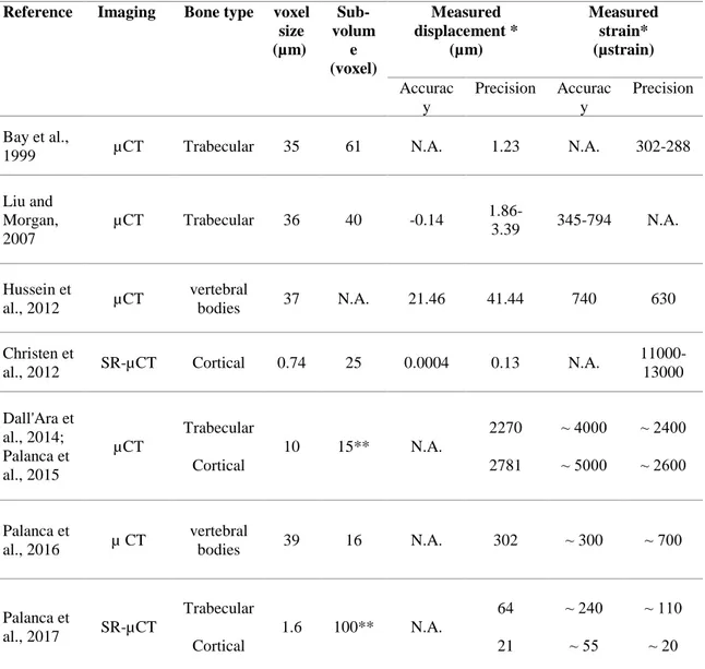
The accuracy and the precision of the DVC to measure stains were evaluated with a home-written script MatLab R2017b (The MathWorks, Inc.). As mentioned above, the strains are computed at each node of a grid placed across the image (Figure 15). When this grid is created, automatically the first node is placed in the center of the image and then nodes are added at distance proportional to the NS on each direction until one layer of nodes lay outside the image. The origin of the coordinate system is at the top left corner of the image.
Figure 15: Schematic representation of the homogeneous cubic grid with a certain nodal spacing (NS) superimposed to one input image (2D representation).
When the image is virtually compressed, in order to replace the moved bone tissue, black voxels have been added in the planes perpendicular to the deformation direction (Figure 17). For this reason, before quantifying the errors, a procedure of removing layers was adopted in a Matlab script, excluding the nodes in the border which correspond to those positions in the deformed image. In fact, these measures are more influenced by the error, due to the lack of features in the border along the compression direction. In particular, the layers of nodes were removed according to the defined NS in the registration and the level and the direction of the applied compression. The script reads the result file of the strain field compute by Ansys. The result file is composed by different columns; the first one specifies the number of the node of the grid, then the other columns indicate the correspondent six independent component of the strain tensor.
33
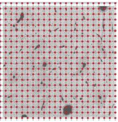
The information of the spatial position of the corresponding nodes of the grid can be read in a different file in which the number of the node is associated with his coordinates, as shown in Figure 16.
Figure 16: Example of the first lines of the output files that contain the numbers of the node (Node) and the coordinates of the nodes (x, y and z). In the same file is also possible read the displacements of each node (u, v and w).
The Nodal Spacing, the voxel size, the number of voxel that composed the VOI and the nominal strain applied must be specified in the script. This allows to exclude the values that correspond to strain measurements in the nodes outside of the bone tissue in the virtually deformed image due to the compression (Figure 17). In case of composed deformation, as the compression has been performed in all the three directions, that procedure has been performed in all the boundaries (Figure 17).
34
Figure 17:On the left side is shown the VOI after 1% of compression along X (represented in 2D and 3D) and after 1% of compression along X, Y and Z. On the right side, the representation of the spatial distribution of the strain measurements (represented in 2D and 3D). The nodes of the border removed along the direction of compression have been highlighted in red.
35
Afterwards, the uncertainties analysis of the DVC for strain measurements is performed computing different metrics. First, for each specimen, the systematic and random error were quantified for each component of strain as in (Gillard et al., 2014; Palanca et al., 2015; Palanca et al., 2016; Tozzi et al., 2017; Palanca et al., 2017). This type of analysis is conducted to find out any potential anisotropy in the DVC strain measurements when a deformation is applied. The systematic error for each component of strain has been computed as average of the respective component of strain on the evaluated nodes, subtracting the nominal value. In a similar way, the random error for each component of strain has been calculated as standard deviation of the respective component of strain on the evaluated nodes, subtracting the nominal value. The systematic or random percentage errors have been computed as the percentage ratio between the systematic or random errors computed over the nodes of the DVC grid and the nominal applied deformation.
In order to allow the comparison between this work and other study in the literature, two different metrics were used to account simultaneously for the errors along the six independent components of strain: the mean absolute error (MAER) and the standard deviation of the error (SDER). The first one, referred as “accuracy” in (Liu and Morgan, 2007), is compute as average of the average of the absolute value of the six components of strain in each node.
𝑀𝐴𝐸𝑅 = 1 𝑁∑ ( 1 6∑|𝜀𝑐,𝑘| 6 𝑐=1 ) 𝑁 𝑘=1
Where ɛ𝑐 represents the six independent components of strain and N is the number of measurement points. The SDER, referred as “precision” in (Liu and Morgan, 2007), is calculated as standard deviation of the average of the absolute values of the six components of strain in each node.
𝑆𝐷𝐸𝑅 = √1 𝑁∑ ( 1 6∑|𝜀𝑐,𝑘| 6 𝑐=1 − 𝑀𝐴𝐸𝑅) 2 𝑁 𝑘=1
36
In this study, the results are reported as median and standard deviation of the errors computed among the values found for the four specimens for each component of strain. The frequency plots have been represented for each component of strain and each specimen in order to evaluate the peaks and the tails in the strain distribution and give a first estimation of either systematic and random errors. Moreover, to assess the effect of the NS on the DVC uncertainties, the trend of the systematic and random errors in function of different NS have been shown in the results.
The spatial distribution of the six strain components in different section planes of each VOIs has been analyzed with Ansys Workbench post-processing functions. This allowed to locate any error concentration inside the specimens.
Lastly, as a further evaluation of the uncertainties, more layers of nodes have been removed from the strain measurements along the deformation direction (Figure 18). Trends of the systematic and random error of the strain components have been reported in function of the number of levels of nodes removed from the border.
Figure 18: Layers of nodes in the border removed from the uncertainties analysis have been highlighted in red. Here the deformation was along Y. Instead, the blue
37
3. Results
3.1 Frequency plot
The normal and shear strain components distributions (EPELX, EPELY, EPELZ, EPELXY, EPELYZ and EPELXZ) for different directions (X, Y and Z) and level (1%, 2% and 3%) of virtual deformation have been visualised out for all the specimens. The frequency plot of the nominal strain components, along the direction of deformation showed a more pronounced peak in the nominal strain and, for the other deformation directions, the peaks were located around 0 microstrain (Figure 19, Figure 20 and Figure 21). Moreover, the shape of the distribution was more symmetric in the components where no deformation is applied. Shorter peaks at higher strain value were observed in the strain distributions for the components along the deformation direction.
Along one deformation direction, the frequency plot of the normal strain components highlights the shift of the central peak towards the increasing the level of deformation (1%, 2% and 3%) (Figure 22, Figure 23, Figure 24). Similar trends have been obtained in the frequency plot of the strain components in all the specimens used. For this reason, only one case has been reported here (Specimen 2).
Figure 19: Frequency plot of the normal strain component along X in the Specimen 2 for 1% of deformation along X, Y and Z. The results for the other specimens showed similar trends. The black vertical lines highlight the nominal virtual deformation applied on the strain component considered.
38
Figure 20:Frequency plot of the normal strain component along Y in the Specimen 2 for 1% of deformation along X, Y and Z. The results for the other specimens showed similar trends. The black vertical lines highlight the nominal virtual deformation applied on the strain component considered.
Figure 21:Frequency plot of the normal strain component along Z in the Specimen 2 for 1% of deformation along X, Y and Z. The results for the other specimens showed similar trends. The black vertical lines highlight the nominal virtual deformation applied on the strain component considered.
39
Figure 22:Frequency plot of the normal strain component along X in the Specimen 2 for 1%, 2% and 3% of deformation along X. The results for the other specimens showed similar trends. The black vertical lines highlight the nominal virtual deformation applied on the strain component considered.
Figure 23:Frequency plot of the normal strain component along Y in the Specimen 2 for 1%, 2% and 3% of deformation along Y. The results for the other specimens showed similar trends. The black vertical lines highlight the nominal virtual deformation applied on the strain component considered.
40
Figure 24:Frequency plot of the normal strain component along Z in the Specimen 2 for 1%, 2% and 3% of deformation along Z. The results for the other specimens showed similar trends. The black vertical lines highlight the nominal virtual deformation applied on the strain component considered.
The distributions of the shear strain components (EPELXY, EPELYZ and EPELXZ), for different direction and magnitude of simulated stain, showed a similar pattern (Figure 25, Figure 26 and Figure 27). In fact, in all the shear strain components the frequency plot presented a gaussian distribution shape with a peak collocated approximately in 0 microstrain. The frequency plots were similar almost in all the specimens except for one (Specimen 1) who showed a different pattern only in the XY shear strain component for deformation along X and Y (Figure 28).
41
Figure 25:Frequency plot of the shear strain component along XY in the Specimen 2 for 1%, 2% and 3% of deformation along X (on the top) and along Y (on the bottom).The black vertical line highlights the nominal virtual deformation applied on the strain component considered.
42
Figure 26: Frequency plot of the shear strain component along YZ in the Specimen 2 for 1%, 2% and 3% of deformation along Y (on the top) and along Z (on the bottom). The black vertical line highlights the nominal virtual deformation applied on the strain component considered.
43
Figure 27:Frequency plot of the shear strain component along XZ in the Specimen 2 for 1%, 2% and 3% of deformation along X (on the top) and along Z (on the bottom). The black vertical line highlights the nominal virtual deformation applied on the strain component considered.
44
Figure 28:Frequency plot of the shear strain component along XY in the Specimen 1 for 1%, 2% and 3% of deformation along X (on the top) and along Y (on the bottom).The black vertical line highlights the nominal virtual deformation applied on the strain component considered.
45
3.2 Systematic errors
Median and standard deviation of the systematic error of each component of strain have been evaluated for the four specimens, at every deformation level and direction simulated (Figure 29, Figure 30 and Figure 31). The systematic errors of the normal strain components along the deformation direction were higher compared to the those computed for other strain components, at each deformation level and direction.
The systematic errors of the normal strain component along X were 714±210, 864±193 and 985±131 microstrain for 1%, 2% and 3% of nominal deformation along X, respectively. Systematic errors of 1064±273, 1126±171 and 1091±96 microstrain have been found in the normal strain component along Y for 1%, 2% and 3% of deformation along Y, respectively. Finally, along Z the systematic errors computed for the normal strain component along Z were 775±211, 1036±165 and 974±191 microstrain for 1%, 2% and 3% of deformation, respectively. Lower median errors were found for the components of the strains with nominal values of 0 for tests performed along each normal direction and for each deformation level (range: -160 to 147 microstrain).
Moreover, high values of standard deviation in the shear strain component along XY have been observed, for the tests with simulated deformations along X or Y, at each level tested (Figure 29 and Figure 30). This is mainly due to the high values of uncertainties for one of the specimens (Specimen 1) (see Table 1 in the Appendix).