Thermal rock properties of geothermal reservoirs and caprocks in the Danish Basin – prerequisites for geothermal applications

ALMA MATER STUDIORUM A.D. 1088

UNIVERSITÀ DI BOLOGNA

SCUOLA DI SCIENZE

Corso di Laurea Magistrale in Geologia e Territorio

Dipartimento di Scienze Biologiche, Geologiche ed Ambientali

Tesi di Laurea Magistrale

Thermal rock properties of geothermal reservoirs

and caprocks in the Danish Basin – prerequisites

for geothermal applications

Candidato: Relatore:

Roberto Miele Prof. Marco Antonellini

Correlatore:

Dr. Sven Fuchs

Acknowledgments

First of all, I would like to warmly thank my external supervisor, Dr. Sven Fuchs (GFZ Helmholtz Centre Potsdam), who gave me the opportunity to join his research team and work at the GFZ institute. His patient guidance, enthusiastic encouragement and useful critiques have been essential for the realisation of this work.

I would also like to express my deepest gratitude to Dr. Andrea Förster (GFZ), for the studentship position and for the financing of this project, as well as for the valuable advice she gave me during my time at the GFZ.

Furthermore, my deep gratitude goes to my supervisor Prof. Marco Antonellini (University of Bologna) for his assistance and advice that have been of great importance in the realization of this work.

I am also particularly grateful for the work of Christian Cunow and Matthias Kreplin (GFZ) in sample preparation and for the assistance in all the laboratory procedures. They were always available whenever I needed help or had a question.

Many thanks also to Dr. Ben Norden and Dr. Hans-Jürgen Förster (GFZ) for sharing their knowledge with me and giving me useful advice in several occasions.

I want to thank also my friends and my beloved flatmates, who listened to me while continuously rambling about this dissertation.

Finally, I want to express my very profound gratitude to my parents, Lorenzo and Giuliana, for providing me with unfailing support and continuous encouragement throughout these years of study. My curiosity and interest for science and my love for nature I owe them especially to them.

This accomplishment would not have been possible without all of them. Thank you.

Table of contents

2.1. Heat Storage 4 2.2. Heat transport 5 3. Overview of the study area ... 6

3.1. Geographical location 6 3.2. Geology 7 3.2.1. Tectonic setting 7 3.2.2. Evolution of the Norwegian-Danish Basin 8 3.2.3. Late Triassic – Early Cretaceous lithostratigraphy 10 3.2.3.1. Gassum Formation 11 3.2.3.2. Fjerritslev Formation 12 3.2.3.3. Haldager Sand Formation 13 3.2.3.4. Flyvbjerg Formation 14 3.2.3.5. Børglum and Frederikshavn Formations 14 3.2.3.6. Cretaceous Chalk Members and Neogene sedimentation 15 3.3. Geothermics 16 3.3.1. Potential reservoirs in the Danish Basin 16 4. Material and methods ... 18

4.1. Samples compilation 18

4.1.1. Aars-1 18

4.1.2. Farsø-1 20

4.1.3. Stenlille-1 22

4.1.4. Lavø-1, Sæby-1 and Gassum-1 samples 23

4.1.5. Classification by major components 24

4.2. Laboratory analyses 25

4.2.1. Drying process 26

4.2.2. Saturation procedure 27

4.2.3. Archimedes’ method 28

4.2.4. Optical Scanning method 29

4.2.4.1. Theoretical background 29

4.3. Data processing 34

4.3.1. Geometric mean model 34

4.3.2. Final data set 36

4.3.3. Software 36

5. Results ... 37

5.1. Petrophysical properties and lithology 37

5.1.1. Porosity and density 37

5.1.2. Bulk thermal conductivity and bulk thermal diffusivity 40

5.1.3. Specific heat capacities 43

5.1.4. Anisotropy 44

5.1.5. Geometric mean model application on bulk thermal properties 45 5.1.6. Matrix thermal properties from geometric mean model 48

5.2. Characteristics by formations 50

6. Discussions and conclusions ... 53

6.1. Bulk thermal diffusivity and geometric mean model 53 6.2. Matrix thermal properties as indicators of the composition of the rocks 55 6.3. Variability of the investigated properties and comparison with literature 57 6.3.1. Variability within the Danish Basin 57

6.3.2. Variability with saturating fluid 60

6.4. Summary of the main results 62

Appendix A ... 64 Appendix B ... 65 References ... 66

Abstract in Italian

Il sottosuolo danese offre un grande potenziale per l'utilizzo del calore geotermico a bassa entalpia e, quindi, per modificare la struttura di teleriscaldamento nazionale, fornendo un carico di base al sistema. Nell'ultimo decennio sono state condotte nuove campagne di esplorazione e ricerca per rimuovere gli ostacoli geologici, tecnici e commerciali per un uso significativo di queste risorse geotermiche. Uno degli ostacoli principali è la conoscenza delle proprietà termiche delle rocce quali conduttività, diffusività e capacità termica. Le condizioni termiche del sottosuolo, nonché la capacità produttiva e il ciclo di vita degli impianti di teleriscaldamento geotermico dipendono in gran parte, tra gli altri parametri, da queste proprietà. Per il bacino danese in particolare sono disponibili solo pochi set di dati pubblicati e quasi totalmente limitati alla conduttività termica delle rocce. I valori di diffusività termica e calore specifico sono in gran parte sconosciuti. Per superare questa lacuna, sono state effettuate nuove misurazioni di laboratorio. La conduttività termica e la diffusività termica sono misurate su sezioni di carota, mentre il calore specifico è calcolato in base a questi valori e alla densità della roccia. Gli obiettivi geologici dello studio sono le arenarie del bacino del Mesozoico (Formazioni del Gassum, Frederikshavn e Haldager Sand), così come rocce argillose e calcari appartenenti a formazioni che fungono da caprocks (Formazioni di Fjerritslev, Vedsted e Unità Gessose). La suite di 43 campioni studiata comprende rocce di sei pozzi: Aars-1, Farsø-1, Stenlille-1, Lavø-1, Gassum-1 e Sæby-1. Le misurazioni sono eseguite su rocce secche e sature in acqua pura, utilizzando il metodo di scansione ottica (Thermal Conductivity Scanner, Popov et al., 1999). Inoltre, sono ricavati i valori di conduttività e diffusività termica di matrice attraverso l’utilizzo del modello di media geometrica. Pertanto sono individuati i range di valori caratteristici per ogni litologia e viene fornita un’indagine qualitativa sulla composizione mineralogica dei campioni sulla base dei dati di matrice. Ulteriori osservazioni sono fatte sul comportamento della diffusività termica e l’applicazione relativa della modello di media geometrica.

Questo studio è stato reso possibile grazie al supporto del progetto "GEOTHERM", finanziato dalla Innovation Fund Denmark.

Parole chiave: bacino danese, conduttività termica, diffusività termica, capacità termica, optical scanning, geotermia a bassa entalpia, GEOTHERM.

Abstract in English

The Danish subsurface provides a large potential for the use of low-enthalpy geothermal heat and, thereby, to change the national district heating structure by providing a base load power to the system. In the past decade, new exploration and research campaigns were performed to remove geological, technical and commercial obstacles for a significant use of these geothermal resources. One of the obstacles is the lack of knowledge on the thermal-related physical rock properties. Subsurface thermal conditions as well as the production capacity and lifecycle of geothermal district heating plants largely depend, among other parameters, on these properties. For the Danish Basin only few published data sets are available and mostly limited to thermal conductivity. Values of thermal diffusivity and specific heat capacity are mostly unknown. In order to overcome this gap, new laboratory measurements were conducted. Thermal conductivity and thermal diffusivity were measured on drill cores sections, while specific heat capacity was calculated based on these values and on rock density. Geological targets for the study are Mesozoic reservoir sandstones (Gassum Fm., Frederikshavn Fm., Haldager Sand Fm.), but also mud-/claystones and limestones of seal rocks (Fjerritslev Fm., Vedsted Fm.). The rock suite of 43 specimens studied was sampled in six wells: Aars-1, Farsø-1, Stenlille-1, Lavø-1, Gassum-1 and Sæby-1. The measurements are performed under dry and saturated conditions using the optical scanning method (Thermal Conductivity Scanner; Popov et al., 1999). Furthermore, the values of conductivity and thermal diffusivity of the matrix were obtained by geometric mean averaging. Therefore, the ranges of characteristic values for each lithology were identified and a qualitative survey on the mineralogical composition of the samples on the basis of the matrix data was assembled. Further observations on the behaviour of thermal diffusivity and the relative application of the geometric mean model are also provided.

This study was possible thanks to the "GEOTHERM" project, funded by the Innovation Fund Denmark.

Keywords: Danish Basin, thermal conductivity, thermal diffusivity, specific heat capacity, optical scanning, low enthalpy geothermal, GEOTHERM.

1. Introduction

The reduction of CO2 emissions in the atmosphere and limitation of fossil fuel usage is a

key global issue. Therefore, the general interest in using renewable energy sources is constantly growing. Geothermal systems represents a fundamental element for this goal, as they can be used for different applications (from energy production to storage of gas or energy itself). More than one hundred geothermal plants are currently operating in the European territory and this number is destined to grow in the next years (EGEC, 2017).

Denmark, is investing in this field, in order to become entirely based on green energy. Currently, geothermal energy plays an important role in district heating systems and gas storage in this country. As pointed out by several authors (e.g. Balling, 1992; Nielsen et al., 2004; Mahaler & Magtengaard, 2010; Mathiesen et al., 2010), the Danish subsurface is currently not believed to be sufficiently efficient for direct electricity production, mainly due to the low permeability of the deeper and warmer aquifers. Nonetheless, the basin has a great potential in terms of low-enthalpy. Moreover, increasing technologies and research may lead to the production of electricity from these systems in the future (van Wees et al., 2013; Røgen et al., 2015). Past and recent research is focused on the characterization of petrophysical and geochemical properties of sandstone reservoirs in geothermal systems and the definition of their spatial distribution in the basin. Particular interest was focused on the Jurassic and Triassic formations, where several units were identified as potential reservoir originally by Balling et al. (1981) and Balling et al. (1992):

 Frederikshavn Member (Upper Jurassic);  Haldager Sand Member (Middle Jurassic);

 Gassum Formation (Upper Triassic - Lower Jurassic);  Skagerrak Formation (Lower to Upper Triassic);  Fjerritslev Formation (Middle Triassic);

 Bunter Sandstone Formation (Lower Triassic).

These Mesozoic formations are related to two Permian–Cenozoic tectonic structures, which extend in northern Europe: the Norwegian-Danish Basin and the North German Basin.

Three geothermal plants are already in operation in Thisted, Copenhagen and Sønderborg, while several other sites are under investigation for the construction of new plants (Danish Energy Agency, 2014). The first geothermal heating plant started the production in Thisted in 1984. The heat is produced using 15 % saline water at 43 °C, taken from the Gassum Formation at a depth of 1.25 km. Currently, the plant has a capacity of 7 MWt (75 TJ/yr). The second plant is located in Copenhagen (Margretheholm). It takes water from a well at 2.6 km of depth from the Bunter Sandstone reservoir. The water has a salinity of 19 % and a temperature of 74 °C. The production of the plant started in 2005 and currently produces 14 MWt (180 TJ/yr). The latest plant, at up to 12 MWt (100 TJ/yr) started production at Sønderborg in 2013. It uses water at 48°C from 1.2 km depth, from Gassum Formation. The salinity of the water is 21 % (Mahler & Magtengaard, 2010; Røgen, et al., 2015). These plants have one injection well producing heat through a heat exchanger and/or based absorption heat pumps. The driving heat primarily comes from external sources (such as biomass boilers). Considering the shallow geothermal heat production (around 27,000 installation), the total installed capacity of the country is 353 MWt, with an annual energy use of 3,755 TJ/yr (Røgen, et al., 2015).

1.1. GEOTHERM project

The first studies on detailed reservoir extension, reservoir properties and temperatures on regional scale were carried since the 1970s. The Dansk Olie & Naturgas A/S (DONG A/S) and the Geological Survey of Denmark and Greenland (GEUS; former “DGU”) were involved in exploration, research, advisory and consultancy for geothermal energy in Denmark.

The GEOTHERM project is an on-going multi-disciplinary research project, carried out jointly by GEUS (as coordinator of the project), the University of Aarhus, the Geological Survey of Sweden, the German Research Centre for Geosciences (GFZ), and the DONG Energy. This project aims to remove remaining geological, technical and commercial obstacles, by analysing in details the Danish subsurface. Properties such as depth to reservoir, thickness, permeability and temperature of geothermal reservoirs were analysed, combining new data with those already available. In particular, one of the main project goals is to study and investigate petrophysical rock properties of major geothermal reservoir sandstones and adjoining cap rocks. A second aim is to identify the variability of these properties according to the lithological composition and to determine the geological formations that are most suitable for geothermal applications. The final goal is the production of geological and geophysical models, for the understanding of lateral and vertical variations in reservoir quality and temperature.

1.2. Aim of this study

The work herein presented reflects parts of the Work Package 4 of the GEOTHERM project and consists in the measurement and investigation of the petrophysical properties of 42 drill-core samples, collected from six wells of the Danish onshore (Aars-1, Farsø-1, Stenlille-1, Lavø-1, Sæbey-1 and Gassum-1). Most of the analysed rocks belong to the Mesozoic formations of the Danish Basin: Gassum, Fjerritslev, Haldager Sand, Flyvbjerg, Frederikshavn, and Vedsted Formations. A smaller part of the collection represents the Upper Cretaceous chalk units, which was sampled in the adjacent Skagerrak–Kattegat Platform.

The last petrophysical data of the sedimentary units in the Danish Basin date back to 1992 (Balling et al., 1992) and are representative of wide depth intervals within the basin. This work contributes to the resolution of this problem by providing new results from detailed laboratory analyses. A thermal characterization of the specimens is provided, including bulk thermal conductivity and bulk thermal diffusivity, measured at ambient conditions, using the Optical Scanning method (Popov et al., 1999). The samples were analysed in dry and saturated conditions. Moreover, effective porosity and density of each sample were defined through the Archimedes method. Secondly, the geometric mean model (Woodside &

Messmer, 1961a,b) was applied for the calculation of matrix thermal properties and

conversion of the bulk values. Such parameters underpin the numerical modelling for the geothermal potential of the Danish Basin, which will be computed by the colleagues from Aarhus University in a subsequent Work Package of the GEOTHERM project.

The main objective of this work is the investigation of the relationships between rock type and their thermal properties. In particular, the variations of these characteristics with the lithology, main mineralogical components and porosity were examined, in order to define the characteristic ranges. Finally, the measurements here presented were compared with the data available in the literature, in order to evaluate the variability of these properties within the Danish Basin.

This thesis is organized in six chapters, as follows:

1. Introduction (current chapter).

2. Theoretical framework: this chapter provides a brief outline of the thermal

parameters investigated, focusing the attention on the underlying theory.

3. Overview of the study area: the geographical location of the wells from which the

rock samples are collected is described. Moreover, the tectonic and sedimentary context in which these rocks formed are outlined. Finally, the attention is focused on the thermal regime of the Danish territory and the geothermal systems currently used.

4. Material and methods: In this chapter the samples taken under examination are first

listed and described. Subsequently, all laboratory procedures and data analysis are described, briefly integrating the underlying theory.

5. Results: all results achieved in the measurement phase of the petrophysical

properties and data analysis are shown here.

6. Discussion and Conclusions: the main results obtained in this thesis are analysed

and discussed here, including a comparison with the available literature. The chapter ends with a brief summary of the results achieved in this work.

2. Theoretical framework

Variations in the temperature field are generally linked to the variation of terrestrial heat flow, the thermal conductivity, stratigraphy, and the radioactive-heat sources in the basin. For geothermal modelling, it is fundamental to define different thermal properties of the Earth subsurface. For this purpose, two main characteristics of a geothermal system are investigated: how the heat is absorbed and how it is transferred within the rocks of the system. In the first case, it is necessary to quantify the heat capacity of reservoirs and contiguous cap rocks. In the second case, thermal conductivity, thermal diffusivity and heat flow density are the main parameters to define (e.g. Clauser, 2006; Fuchs & Förster, 2010; Fuchs et al., 2015). These properties vary both laterally and with depth, depending on several factors such as petrography and porosity of the rocks, the saturating fluids in pores and fractures, tectonic setting of the area, and paleoclimate history. For a more detailed dissertation on this topic, see e.g. Clauser (2006, 2009, 2011) and Robertson (1988).

2.1. Heat Storage

The heat capacity C quantifies the amount of heat that can be stored in a rock volume. It is determined by the amount of heat (ΔQ) required to raise the temperature of a body by (ΔT).

𝐶 =𝛥𝑄

𝛥𝑇 [

𝐽

𝐾] (1.1)

When considering a unit mass (M) of a substance, the specific heat capacity c is defined.

𝑐 = 𝛥𝑄

𝑀 ∗ 𝛥𝑇 [

𝐽

𝑘𝑔 ∗ 𝐾] (1.2) In geothermal modelling, it is useful to consider isobaric specific heat capacity (cp). As

defined e.g. by Clauser (2006), this parameter can be inferred considering the following state function for a closed system

𝑑𝐻(𝑃, 𝑇) = 𝑑𝐸 + 𝑃𝑑𝑉 + 𝑉𝑑𝑃 [𝐽] (1.3) where the variation of the enthalpy of the system (dH) is given by variation of internal energy (dE) and work (PdV + VdP). Assuming dE as the sum of change in heat (dQ) and the work delivered to the system (dW), and dW as only volume expansion work

𝑑𝐸 = 𝑑𝑄 + 𝑑𝑊 [𝐽] (1.4)

𝑑𝑊 = −𝑃𝑑𝑉 [𝐽] (1.5)

it is finally possible to define the isobaric specific heat capacity as 𝑐_𝑃 = 𝑑𝑄 𝑑𝑇 = ( 𝜕𝐻 𝜕𝑇)_𝑃 [ 𝐽 𝐾] (1.6)

Thus, isobaric specific heat capacity is the first derivative of enthalpy with respect to temperature. Finally, by comparing equations (1.2) and (1.6) it is possible to settle their

𝑐_𝑃 = 𝛥𝐻 =𝛥𝑄

𝑀 [

𝐽

𝑘𝑔 ∗ 𝐾] (1.7) Nonetheless, the total heat capacity of a rock is defined by heat capacities of both rock and saturating fluids in pores and fractures. Thus, a common way to calculate the heat capacity is on a volumetric basis, using the volumetric heat capacity (or thermal capacity) ρc.

𝜌𝑐 = 𝜆/𝛼 [ 𝐽

𝑚3 _{∗ 𝐾}] (1.8)

where ρ is the density in kg/m³, λ is the thermal conductivity in W/(m*K) and α is the thermal diffusivity [m2_{/s] (see the following section) of the specific phase considered. Moreover, the}

difference between isobaric and isochoric specific heat capacity is negligible for crustal rock at temperatures below 1000K.

2.2. Heat transport

In Earth’s crust, the heat is transported mainly by diffusion and conduction. Advection occurs only when a sufficiently large hydraulic permeability is available and the contribution of radiation is relevant only when the ambient temperature is greater than ca. 600 °C. Thus to define the transport of heat through a rock, two fundamental parameters must be specified: thermal conductivity and thermal diffusivity.

The thermal conductivity (λ) is an intrinsic physical property of the rocks for steady state conditions. This quantity defines the amount of heat that flows across a unit cross-section of rock, along a unit distance, per unit temperature decrease, per unit time [W/(m*K)].

In transient state conditions, the thermal diffusivity α describes the heat diffusion in a rock. Clauser (2011) defines the thermal diffusivity as “the ratio of heat flowing across the face of a unit volume and the heat stored in the unit volume per unit time” [m2_{/s]. It is also}

possible to define this quantity as the ratio of thermal conductivity and volumetric heat capacity, considering Eq. (1.7).

As previously mentioned, the heat-flow density (qi, later referred to be the “heat flow”)

has a pivotal role for thermal characterization of a site. When observed at the surface, it counts as surface heat flow (qs). When unaffected by paleoclimate, terrain effects such as

heat refraction or similar effects, it counts as terrestrial surface heat flow and reflects the “real” heat flow from the Earth’s interior. For steady state conditions, the heat flow is defined by Fourier’s law

𝑞_𝑖 = 𝜆_𝑖𝑗𝜕𝑇

𝜕𝑥_𝑗 [

𝑊

𝑚2] (1.9)

where (∂T/∂xj) is the thermal gradient vector. The heat flow itself is a vector, depending on

the thermal conductivity tensor (λij). In fact, the layering of sedimentary rocks, as well as the

foliation in general, defines differences of thermal conductivity between the directions parallel and perpendicular to bedding. Thus, the thermal conductivity tensor is related to the anisotropy of the rocks. For isotropic rocks, the heat flow will be predominantly vertical and it is sufficient to consider only its vertical component. On the contrary, for many sedimentary and metamorphic rocks the lateral heat flow is significant, due to their inhomogeneity (Clauser, 2011).

3. Overview of the study area

3.1. Geographical location

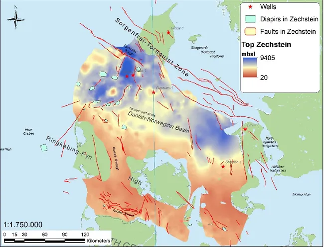
The study area is the Danish Basin, a buried extensional basin that approximately covers the vast majority of the Danish territory, both onshore and offshore. In particular, the samples analysed in this project were collected from six wells shown in Fig. 3.1, in the north-eastern part of Denmark. The names of the wells indicate the six cities in which they were drilled, which are located in the Midjylland (Gassum-1), Norjylland (Farsø-1, Aars-1 and Sӕby-1), Sjӕlland (Stenlille-1) and Hovedstaden (Lavø-1) regions. The wells are in different tectonic structures of the basin, as shown in Fig. 3.2:

 Aars-1, Farsø-1, Gassum-1 and Stenlille-1 are placed in the Danish Basin  Sæby-1 is located on the northern part of the Skagerrak-Kattegat-Platform

 Lavø-1 is located on the Ringkøbing-Fyn High area in the South Such tectonic structures are described in the following paragraph.

Figure 3.1: Area of interest of this work. The red stars represent the location of the wells from which the samples of this work were collected (Coordinate System: ED50/UTM Zone 32). Data: GEUS.

3.2. Geology

3.2.1. Tectonic setting

The Danish Basin constitutes the eastern part of the Norwegian-Danish Basin, comprising the Danish Embayment and the Danish Sub-basin. It is an intra-cratonic, Permian–Cenozoic structure, trending WNW–ESE (Michelsen et al., 2003; Michelsen & Nielsen, 1993; Nielsen, 2003). The Norwegian-Danish Basin, in turn, belongs to the eastern part of the North Sea Basin, which is made up of several fault-bounded basins, interspersed with structural highs (Balling, 1992). Five major structural elements, generally oriented NW–SE, are distinguished in the study area (Fig. 3.2):

 The North German Basin and the Ringkøbing–Fyn High to the south  The Danish Basin

 The Sorgenfrei–Tornquist Zone and the Skagerrak–Kattegat Platform to the north-east

The Ringkøbing-Fyn High separates the Danish Basin from the Northern German Basin. It consists of shallow faulted blocks of Precambrian basement. To the northeast, the Skagerrak–Kattegat Platform and the Sorgenfrei–Tornquist Zone separate the basin from the Precambrian Baltic Shield and together constitute the Fennoscandian Border Zone (EUGENO-S Working Group, 1988; Michelsen et al., 2003; Nielsen, 2003). The Sorgenfrei-Tornquist Zone is a block-faulted zone, 30–50 km wide, with tilted Palaeozoic rocks. It runs from the North Sea in the Skagerrak area to the Rønne Graben in the Baltic Sea and

the Late Carboniferous – Early Permian times and defines a rift zone. The adjacent and eastern Skagerrak-Kattegat Platform is a more stable area composed by Lower Permian, Lower Palaeozoic and Precambrian crystalline rocks (EUGENO-S Working Group, 1988; Nielsen, 2003; Vejbӕk, 1989).

The syn-rift succession is separated from the post-rift one by a basin-wide unconformity: the pre-Zechstein surface. It mainly covers Precambrian crystalline rocks on the Ringkøbing–Fyn High and Skagerrak–Kattegat Platform and lower Palaeozoic deposits in most of the Danish Basin and Sorgenfrei–Tornquist Zone. Eventually, Late Carboniferous – Early Permian syn-rift clastic rocks (Rotliegend group) are found under this unconformity (Michelsen & Nielsen, 1993; Nielsen, 2003). The Upper Triassic – Jurassic succession is 5 – 6.5 km thick along the Danish Basin and more than 9 km thick in the Sorgenfrei– Tornquist Zone. It is possible to distinguish two main tectono-stratigraphic units, separated by an intra-basinal unconformity:

 The Norian – Lower Aalenian succession, formed under relative tectonic tranquillity. In this succession, the sediments are relatively undisturbed and define a layered-cake geometry, except for areas where local faulting or diapir movements occurred. The sedimentation is mainly controlled by sea level changes;

 The Late Middle – Jurassic succession, influenced by a fault controlled subsidence and sea level changes.

These deposits represent various environments, from dominantly fluvial to paralic and coastal in the east, to deep marine in the west (Michelsen et al., 2003; Nielsen, 2003). According to the EUGENO-S working group (1988), the crustal thickness variates between 28 and 30 km in the Norwegian-Danish Basin and Sorgenfrei–Tornquist Zone, whereas it is 32–36 km thick in the Skagerrak-Kattegat Platform and Ringkøbing–Fyn High.

3.2.2. Evolution of the Norwegian-Danish Basin

The formation of the Norwegian-Danish Basin is caused by regional thermal cooling that followed a Late Carboniferous – Early Permian rifting phase. Erosion followed the rifting, causing the formation of the top pre-Zechstein surface (EUGENO-S Working Group, 1988; Michelsen & Nielsen, 1993; Vejbæk, 1989). A marine transgression in the Upper Permian led to the deposition of thick layers of calcareous and salt deposits (Zechstein Formation) in the central part of the basin. The halokinetic movements of the Zechstein’s salt influenced the geometry and the sedimentation of the following successions (Nielsen 2003; Petersen et al., 2008; Vejbæk, 1989).

From Lower to Middle Triassic, thick layers of mainly continental sediments were deposited (Michelsen & Nielsen, 1993; Nielsen 2003; Petersen et al., 2008). The Norian stage is characterised by the beginning of a transgression phase. The Danish Basin was covered by a shallow marine – paralic environment, which defined the sedimentation of limestones and claystones of the Vinding Formation in the central basin and shallow marine sandstones and mudstones of the Skagerrak Formation in the Sorgenfrei–Tornquist Zone. A regression phase during Rhaetian times caused the coastal progradation and the deposition of mainly shallow marine to fluvial sands towards the centre of the basin, defining the Gassum Formation.

In the earliest Hettangian, a new transgressive phase defined the deposition of marine muds of the Fjerritslev Formation (FI member) in the southwest and the regression of the coastline towards north-east (Fig. 3.3). The Gassum Formation was progressively overstepped until the earliest Sinemurian, when the open marine environment took over in the Sorgenfrei–Tornquist Zone. An overall sea level rise, interspersed by smaller sea level

members of the Fjerritslev Formation (Michelsen et al., 2003; Nielsen, 2003; Petersen et al., 2008). During Aalenian – Bajocian, a regional uplift influenced the Ringkøbing-Fyn High and the Danish Basin. The Triassic – Lower Jurassic succession in the Ringkøbing-Fyn High was totally eroded, as well as part of the Fjerritslev Formation in the Danish Basin. The Sorgenfrei–Tornquist Zone continued to subside at a slower rate, permitting the deposition of the FIV member. A regressive phase during Upper Aalenian defined the deposition of paralic and fluvial sands of the Haldager Sand Formation (Fig. 3.3; Michelsen & Nielsen, 1993; Mogesen & Korstgård, 2003; Nielsen, 2003). The uplift was followed by a regional subsidence that lasted until Volgian times and the Fennoscandian Border Zone was characterized by shallow marine to non-marine environments, and was strongly influenced by repeated transgressive– regressive cycles.

The Oxfordian Age is characterised by the deposition of offshore clay-dominated deposits in the basin, while lagoonal deposition dominated the remaining highs (Flyvbjerg Formation). The deposition of marine claystones of the Børglum Formation followed in the Kimmerdigian. The Frederikshavn Formation was deposited in Volgian– Ryazanian times, in a shallow marine to offshore environment. Non-marine conditions prevailed in the Skagerrak– Kattegat Platform and Sorgenfrei-Tornquist Zone in this period (Michelsen et al., 2003; Petersen et al., 2008). The expansion of the marine environment in Early Cretaceous times caused a deposition of marine mud over most of the study area. The tectonic tranquillity ended during Late Cretaceous–Palaeogene times, giving way to an inversion in the Sorgenfrei– Tornquist Zone. Significant uplift and erosion occurred over parts of the Norwegian-Danish Basin and the Ringkøbing-Fyn High in the Neogene (Michelsen & Nielsen, 1993; Mogesen & Korstgård, 2003; Petersen et al., 2008).

Figure 3.3: Environmental succession of the Norwegian-Danish Basin pre, during and post Middle Jurassic uplift (modified from Michelsen et al., 2003).

3.2.3. Late Triassic – Early Cretaceous lithostratigraphy

In the Norwegian-Danish Basin, the Zechstein evaporites (Fig. 3.4) represent the first post-rift deposit. This succession is present at various depths due to the salt movements. During Early – Middle Triassic, the depositional environment was mainly continental, controlling the deposition of Bunter Sandstone, Skagerrak, Ørslev, Falster and Tønder Formations. See e.g. Petersen et al. (2008) for a more detailed description of these formations and their relative depositional environments. In Norian Age, 40–90 m of marls and oolitic carbonates were deposited, defining the Vinding Formation. (Nielsen, 2003; Petersen et al., 2008). The Upper Triassic – Jurassic succession of the Danish Basin includes Skagerrak, Vinding, Gassum, Fjerritslev, Haldager Sand, Flyvbjerg, Børglum and Frederikshavn Formations (Michelsen et al., 2003; Nielsen, 2003; Petersen et al., 2008).

Figure 3.4: Extension and depth of the top of the Zechstein units, including main faults and salt diapirs that occur within the surface (Coordinate System: ED50/UTM Zone 32). Data: GEUS.

3.2.3.1. Gassum Formation

The Gassum Formation formed during Late Norian – Rhaetian times over most of the basin (Fig. 3.5). Its upper limit is dated to the latest Rhaetian over most of the central part of the Danish Basin, and it progressively youngs to earliest Sinemurian Age towards the Fennoscandian–Border Zone. It interfingers with the Vinding Formation at its base, and its upper part (in the north-eastern part of the basin) is contemporaneous to the FIa member of the Fjerritslev Formation (Michelsen et al., 2003; Nielsen, 2003). In general, the thickness of the formation is between 50 and 150 m in the Danish Basin and between 170 and 200 m in the Sorgenfrei-Tornquist Zone. The maximum thickness of 300 m is reached in this fault bounded area. The Gassum Formation occurs throughout most of Denmark at typical depths of 2,500–3,000 m. Locally, the depth can increase to 2,000–4,000 m. Along the structural highs it is found at 500–1,000 m depth (Balling, 1981). The lithology consist of interbedded white-grey and fine- to medium- grained (occasionally coarse-grained and pebbly) sandstones, greenish-grey heteroliths, mudstones, dark mudstones and few beds of coal. The general porosity of the sandstones is 15–25 % (Michelsen et al., 2003; Nielsen, 2003; Petersen et al., 2008). The formation presents the evidence of repeated sea level fluctuation that strongly influenced the sedimentation, which occurred in a fluvio-deltaic to tidally influenced shallow marine environment (Nielsen, 2003).

Figure 3.5: Extension and depth of the top of the Gassum Formation in the Danish Basin, including main faults and salt diapirs that occur in the formation (Coordinate System: ED50/UTM Zone 32). Data: GEUS.

3.2.3.2. Fjerritslev Formation

The Fjerritslev Formation (Fig. 3.6) overlies the Gassum, generally presenting an abrupt shift. The Aalenian–Bajocian erosion altered the original thickness of the succession. The maximum thickness of 1,000 m is recorded in the Fjerritslev Trough. Locally the formation includes mudstones of latest Rhaetian and Early Aalenian age (Michelsen & Nielsen, 1993; Michelsen et al., 2003; Nielsen, 2003). The formation is subdivided into four informal members (FI – FIV), the lowermost of which can be subdivided into two units, FIa and FIb. It consists in a relatively uniform succession of marine, dark grey to black, slightly calcareous claystones, with a varying content of silt and siltstone laminae. On the Skagerrak– Kattegat Platform, siltstones and fine-grained sandstones form a minor portion of the succession. Around 20–30 m of fine-grained muddy sandstones dominate the F-II member, located on the Skagerrak-Kattegat Platform. They have a porosity of 10–25 % and are frequently interfingered with mudstones. These sandstones were deposited during different sea level minor fluctuations (Michelsen et al., 2003; Nielsen, 2003; Petersen et al., 2008).

Figure 3.6: Extension and depth of the top of the Fjerritslev Formation, including main faults and salt diapirs that occur in the formation (Coordinate System: ED50/UTM Zone 32). Data: GEUS.

3.2.3.3. Haldager Sand Formation

The Haldager Sand Formation (Fig. 3.7) was deposited in a Bajocian–Bathonian period in the Danish Basin and from Aalenian to Callovian in the Sorgenfrei-Tornquist Zone (Michelsen & Nielsen, 1993; Michelsen et al., 2003; Nielsen, 2003). The formation is distributed in the central and northern part of the Danish Basin (restricted to North Jylland), in the Sorgenfrei-Tornquist Zone and on the Skagerrak-Kattegat Platform. The lateral continuity, the thickness and the facies are significantly altered where the salt structures occur. In the Danish sub-basin, the top of the Haldager Sand Formation reaches depths of 2,000–3,000 m. The thickness of the formation is 15–50 m in the Skagerrak-Kattegat Platform, 30–175 m in the Sorgenfrei-Tornquist Zone, and 25–50 m in the central part of the basin. The distribution in the south-western area is patchy and reduced to less than 10 m. The formation is absent on and along the Ringkøbing–Fyn High. This formation consists of light olive-grey, fine- to very coarse grained, occasionally pebbly sandstones, siltstones, mudstones and coaly beds. The sandstones are generally well sorted and their porosity variates between 15 and 30 %. In the Sorgenfrei–Tornquist Zone, the formation is made of thick fluvial-estuarine and marine sandstones separated by marine and lagoonal-lacustrine mudstones. In the south-western part of the basin the formation is characterized by sandstones of braided rivers, 1–10 m thick (Michelsen et al., 2003; Nielsen, 2003; Petersen et al., 2008).

Figure 3.7: Extension and depth of the top of the Haldager Sand, including main faults and salt diapirs that occur in the formation (Coordinate System: ED50/UTM Zone 32). Data: GEUS.

3.2.3.4. Flyvbjerg Formation

Both the base and top of the Flyvbjerg Formation are diachronous all over the basin, younging towards the north-eastern margin. It was deposited from Middle Oxfordian to Late Kimmerdigian. The formation extends from the central basin to the northern part of the Danish Basin and on the Fennoscandian Border Zone (approximately the same distribution as the Haldager Sand Formation). It forms a wedge thickening north-eastward. Maximum thicknesses of 50 m are found over the Fennoscandian Border Zone. It consists of lightly coaly sandstones and siltstones in its lower part. The sediments trend to a more calcareous sandstones interbedded with claystones. In the upper part, fine-grained calcareous sandstones dominate the formation. The succession formed in a shallow to deep marine environment (Michelsen et al., 2003; Nielsen, 2003; Petersen et al., 2008).

3.2.3.5. Børglum and Frederikshavn Formations

The lower boundary of the Børglum Formation is located at the top of the thick sandstone beds uppermost in the Flyvbjerg Formation. This formation consists of a relatively uniform succession of slightly calcareous, homogeneous claystones and mudstones, with varying contents of silt, mica and pyrite. The sediments were mainly deposited in an offshore marine environment. The transition from the claystones of the underlying Børglum Formation to the more coarse-grained Frederikshavn Formation is dated Kimmeridgian–Ryazanian. Although, the Frederikshavn is time-equivalent with the upper part of the Børglum Formation in the central and western parts of the Norwegian–Danish Basin (Michelsen et al., 2003; Nielsen, 2003; Petersen et al., 2008).

Figure 3.8: Extension and depth of the top of the Frederikshavn Formation, including main faults and salt diapirs that occur in the formation (Coordinate System: ED50/UTM Zone 32). Data: GEUS.

The Frederikshavn Formation deposited in the north-eastern part of the Danish Basin (Fig. 3.8). It shows large variations in thickness (75–230 m). The maximum thickness recorded is more than 230 m in the Sorgenfrei-Tornquist Zone. The formation consists of siltstones and fine-grained, slightly calcareous, sandstones interbedded with claystones, deposited in a paralic environment (Balling et al., 2002; Petersen et al., 2008).

3.2.3.6. Cretaceous Chalk Members and Neogene sedimentation

The claystones of the Frederikshavn Formation gradually give way to the Lower Cretaceous mudstones of the Vedsted Formation (Fig. 3.9). These mudstones present sandy intercalations (most common towards the northeast) and the entire formation is divided into four depositional units (Petersen et al., 2008; Michelsen & Nielsen, 1993).

Until the Cenomanian-Turonian, marine greensands were deposited in the easternmost part of the basin and within the Fennoscandian Border Zone, whereas intermittent deposition of marls and mudstones occurred in the south-west. In Late Cretaceous – Danian times, a pelagic chalk deposition over the entire study area took place. In the Sorgenfrei–Tornquist Zone, 1.5–2 km of chalk was deposited, while 500–750 m accumulated over the Ringkøbing–Fyn High. Late Cretaceous – Palaeogene inversion and erosion, masks the original thickness of the chalk succession. During the Palaeocene, deep marine sedimentation of fine-grained hemipelagic deposits took place, while in the Oligocene, major clastic wedges began to build out from the Baltic Shield. Coarse-grained sediments reached the southern part of the basin and the Ringkøbing–Fyn High in Neogene times. Up to 500 m of sediments were deposited in the Norwegian–Danish Basin during the Late Miocene and Pliocene. (Petersen et al., 2008).

Figure 3.9: Extension and depth of the top of the Lower Cretaceous, including faults and diapirs within the units. Data: GEUS.

3.3. Geothermics

Over the past four decades, the subsurface temperatures of the Danish Basin were widely investigated. Despite the presence of a homogeneous temperature vertical structure, the basin presents strong lateral variations, up to about 50 °C at 3,000 m of depth (Balling et al., 1981; Balling, 1992). The temperature gradients in the Norwegian-Danish Basin are mainly ranging between 27 and 30 °C/km (Balling et al., 1981; Balling, 1992; Nielsen et al., 2004). In general, temperatures vary from ca. 25–35 °C at 1,000 m, to over 55–75 °C at 2,000 m and 75–105 °C at 3,000 m. The temperature information originates from two sources: borehole temperature and theoretically modelled values. Temperature gradient were determined as mean gradient between surface and the actual depth of BHT information and they were corrected for the effect of paleoclimate and sedimentation (Balling et al., 1981; Balling, 1992).

The heat-flow density usually increases towards shallow depths due to the impact of the rocks radiogenic heat production. In shallow parts of the Danish Basin the heat flow is strongly influenced by paleoclimate temperature variations (i.e. cooling of the last glaciations; Balling, 1992) yielding values of only 35 to 45 mW/m². If this effect is corrected, the so called terrestrial surface heat flow provides the unperturbed heat flow from the Earth interior. Recent studies have provided values of 64–84 mW/m² for the terrestrial surface heat-flow (Nielsen et al., 2017). The temperatures and heat flow at the Moho were estimated, by Balling (1992) at 700–750 °C and 40–45 W/m2_{, respectively.}

3.3.1. Potential reservoirs in the Danish Basin

The thick Mesozoic succession was the target for hydrocarbon exploration since 1935. Data of borehole drillling and seismic campaigns show that the most promising geothermal reservoirs occur within the Triassic – Lower Cretaceous succession in the Danish Basin (Balling et al., 1981; Mathiesen et al., 2010). The principal sedimentary units of interest are the Gassum Formation and the Haldager Sand Formation, as well as the Bunter Formation. Different secondary potential reservoir are also present in the Skagerrak Formation, the F-II member of the Fjerritslev Formation, the Flyvbjerg Formation and Frederikshavn Formation (Balling, 1992; Mathiesen et al., 2010; Mahaler & Magtengaard, 2010; Nielsen et al., 2004; Petersen et al., 2008).

The Gassum Formation is enclosed by the thick marine mudstones of the Fjerritslev Formation. In North Jylland, the highest temperature gradient of this formation is at about 900 m and a reservoir temperature of 70–100 °C was predicted for this area. Lower values (50–70 °C) were predicted for the southern and eastern parts (Balling et al., 1981). The formation is currently used for geothermal energy, at a depth of ca. 1,200 m, in Thisted, northern Jylland and for natural gas storage at 1,550 m, in the Stenlille area

The Haldager Sand reservoir is surrounded by marine mudstones of the Flyvbjerg and Børglum Formations. Sandstones are present in the lower and upper part of the Flyvbjerg Formation and their thickness tend to increase towards the northern and eastern basin margin, where they may form an additional reservoir section (Petersen et al., 2008). The estimated temperature range is about 60–80 °C, with local increase up to about 100 °C, and decreasing to 30–50 °C at the northern margin (Balling et al., 1981).

Another potential reservoir unit is the upper part of the F-II member (Fjerritslev Formation) on the Skagerrak–Kattegat Platform. This unit is made up of muddy sandstones, which show potentially good characteristics along the Skagerrak–Kattegat Platform. The Flyvbjerg Formation contains shoreface sandstones in its lower and upper parts of the Upper Jurassic, thickening northwards. This formation is covered and isolated by its own marine

The depths and the thickness of these reservoirs vary significantly in the basin. The uncertainty on the quality of the reservoir is strictly linked to the permeability, which varies laterally and vertically. Therefore, every reservoir study must be supplemented with specific surveys and local assessments to estimate local production potentials. The porosity of the sandy units in the Danish Basin decrease markedly with depth: from 30–35 % at 500– 1,000 m, to 20–25 % at 2,000 m and 10–15 % at 3,000 m. The brine permeability decreasing trend is linked to decreasing porosity: from 300–3,000 mD for 30 % porosity, to 10–30 mD for 15 % porosity. This reduction is mainly caused by mechanical compaction and the formation of diagenetic minerals that reduce pore volume and pore connections. (Balling, 1992; Mahaler & Magtengaard, 2010; Nielsen et al., 2004). The water salinity shows a general increasing trend of about 10 % / km, but large variations are found (Mathiesen et al., 2010). At depths of about 2000–3000 m regional potential geothermal reservoirs normally show temperatures of 60–100 °C (Balling et al., 1981). Due to the diagenetic cementation and reduced pore space, the depth of exploitable reservoirs is limited to a range of 2.5–3 km. This limits the maximum temperatures to 80–90 °C. Therefore, the possibility of high-enthalpy systems remains precluded (Mahaler & Magtengaard, 2010). However, a general estimation of the geothermal potential is possible considering layers of sandstones at depths of 1,000–2,500 m, which are thicker than 25 m and sufficiently distributed (Nielsen et al., 2004).

4. Material and methods

4.1. Samples compilation

The samples used in this work were originally collected from the six wells reported in

Fig. 3.1, by the GEUS institute. The dataset consists of 43 core sections collected from the GEUS core storage in Copenhagen, by the help of Niels Balling (Aarhus University), Sven Fuchs (GFZ) and Rikke Weibel (GEUS). The samples were later sent to the GFZ institute, where they were catalogued, treated and analysed, following the procedures described in the following paragraph.

The rock samples’ description presented in this paragraph is the result of a visual analysis carried out prior to the laboratory work. Such analysis was improved by comparing it with data from the well reports and the information provided by the GEUS institute.

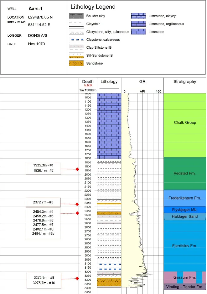
4.1.1. Aars-1

The Aars-1 well (Fig. 4.1) was drilled near the city of Aars (North Jutland) by the Dansk Olie & Naturgas A/S society (DONG A/S) from November 1978 to August 1979. The GEUS provided the well report (GEUS, 1979). The aim of this drilling was to study the prospects of recovering geothermal energy from the Gassum Formation. As shown in Fig. 4.1, 11 samples of the dataset (IDs: 1, 2, 3, 4, 5, 6, 7, 8, 8b, 9 and 10) were collected from this well:  Samples 1 and 2 are representative of the Vested Formation. They appear as dark grey mudstone, slightly shaly, poorly consolidated. Silt is present in very thin layers.  Sample 3 belongs to the Frederikshavn Formation. It is a dark grey, calcareous mudstone, well consolidated. Some calcareous fragments may suggest the presence of mollusc’s fossils.

 Samples 4 and 5 belong to the Flyvbjerg member and consist of grey mudstones with fine-grained sand and a heterolithic bedding.

 Samples 6, 7, 8 and 8b belong to the Haldager Sand. They appear as whitish, medium-coarse grained, homogeneous sandstones. Very small lamellae of dark clay occur sporadically in samples 6 and 7.

 Samples 9 and 10 (Gassum Formation) show contrasting characteristics. Specimen 9 is a dark sandy mudstone, with heterolithic bedding, whereas specimen 10 is a whitish, coarse and very compact sandstone.

Figure 4.1: Log of the Aars-1 well (depth range: 1,000 – 3,400m). This log shows the intercepted lithologies, the GR measures and the relative formations. The red diamonds and the textboxes indicate the depth of each sample (depth [mbKB] - #ID). Data furnished by GEUS.

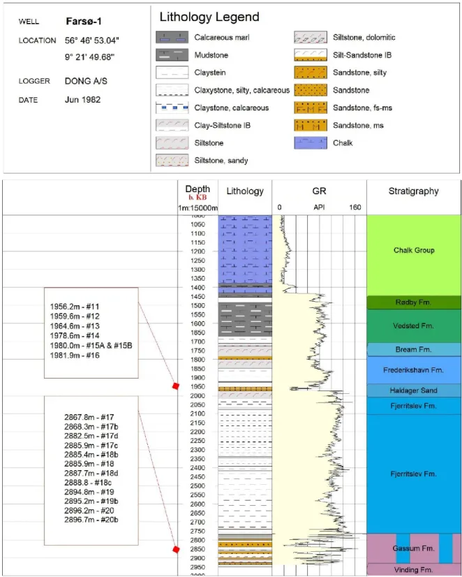
4.1.2. Farsø-1

This well is located in the homonym city of Farsø (North Jutland) and was drilled during 1982 by the DONG A/S and analysed by the GEUS. The aim of this drilling was to evaluate the geothermal potential of the sandy reservoirs, for low enthalpy systems (GEUS, 1982). Nineteen samples of the dataset were collected from this well (IDs: 11, 12, 13, 14, 15A, 15B, 16, 17, 17b, 17c, 17d, 18, 18b, 18c, 18d, 19, 19b, 20 and 20b; Fig. 4.2):

 Samples 11, 12 and 13 are from the Haldager Sand Formation. Specimen 11 is a light grey/yellow very fine-grained sandstone, with silt and dark clay lamellae in thin layers. It is poorly cemented. Specimen 12 is a relatively medium-grained sandstone, with barely evident laminations; specimen 13 is composed by very fine sand and mud intercalated in cross laminations.

 Specimen 14, 15A, 15B and 16 belong to the Fjerritslev Formation. They show similar characteristics: a mainly muddy composition, with barely evident tabular lamination, moderately compacted. Specimen 16 presents some differences: a relatively higher silt composition with a heterolithic bedding.

 The remaining specimens 17, 17b, 17c, 17d, 18, 18c, 18d, 19, 19b, 20 and 20b are all sandy samples belonging to the Gassum Formation. Specimen 17 and 17b are coarse-grained, whitish and homogeneous sandstones. The 17 is poorly cemented. Specimen 17c and 17d are white, fine-grained sandstones with dark mud and tabular (occasionally cross) lamination. The general cementation is good, although the layers of mud may represent weak points. Specimens 18, 18b and 18d are light grey, fine-grained sandstones. Dark mud is present in thin layers. The lamination is generally tabular. They are all well-cemented. In samples 19, 20 and 20b, the lithology is characterized by increasingly coarser sand and thinner mud layers. Sample 18c is the only rock of this group, which is composed mainly by homogeneous, grey mud.

Figure 4.2: Log of the Farsø-1 well between 1,000 and 2,950m depth. This log shows the lithology intercepted, the GR measures and the relative formations. The red diamonds and the textboxes indicate the depth of each sample (depth [mbKB] - #ID). Data furnished by GEUS.

4.1.3. Stenlille-1

This well was drilled in 1981 by the DONG A/S, in the former municipality of Stenlille (now part of the town of Sorø, Zealand). The purpose of this well was to analyse Gassum reservoir and the cap rocks above, in order to investigate the possibility of natural gas storing. Its maximum depth is 1,664 m. The well report is provided by GEUS (GEUS, 1981). Nine of the analysed in total belong to this well (IDs: 21, 22, 23, 23b, 23c, 24, 25, 26 and 26b;

Fig. 4.3):

 Sample 21 is a dark, calcareous and homogeneous claystone. It belongs to the Vedsted Formation.

 Sample 22 is composed of fine-grained sand with a high content in organic mud, poorly cemented.

 Samples 23, 23b and 23c are grey and homogeneous calcareous claystones and belong to the Fjerritslev Formation.

 Samples 24, 25, 26 and 26b belong to the Gassum Formation. sample 24 is a very

Figure 4.3: Log of the Stenlille-1 well between 1,100 and 1,625m depth. This log shows the lithology intercepted, the GR measures and the relative formations. The red diamonds and the textboxes indicate the depth of each sample (depth [mbKB] –#ID). Data furnished by GEUS.

homogeneous, and well cemented sandstones. Samples 26 and 26b sporadically present thin layers of clay.

4.1.4. Lavø-1, Sæby-1 and Gassum-1 samples

The remaining five samples were collected from Lavø-1, Sæby-1 and Gassum-1 wells (respectively GEUS, 1995; GEUS 1985; GEUS 1951). These rocks represent the Cretaceous Chalk Units.

 Samples 27 and 28 consist of white homogeneous calcareous limestones, respectively collected from the Sæby-1 well (at ca. 406 mbKB) and from Gassum-1 well (at ca. 265 mbKB). Both samples have a scarce consistence.

 Samples 29, 30 and 31 are grey limestones with variable presence of dark mud in layers. They were collected from Lavø-1 well (Fig. 4.4). Samples 29 and 30 show a modest lithification and higher content in mud, relatively to 31.

Figure 4.4: Part of the Lavo-1 well log. This log shows the lithology intercepted by the drilling, the GR measures and the relative formations of a depth range from 750 to 2,050mbKB. The red diamonds and the

4.1.5. Classification by major components

The rocks of the compilation were catalogued by their major component into five different classes. Such classification was necessary to evaluate the relations between petrophysical properties and major lithological characteristics, and goes as follows:

I. Sandstones (or ‘Sst’): samples which major component is visibly pure sand;

II. Argillaceous sandstones (or ‘Sst argillaceous’): rocks mainly consisting in

medium-or fine- grained sand with mud. The content in sand is greater than that of mud. A variable content in silt can be present;

III. Sandy mudstones (or ‘Mst sandy’): muddy rocks with a minor but substantial

content in silt or fine sand;

IV. Mudstones (or ‘Mst’): rocks whose major component is pure mud;

V. Limestones (or ‘Lst’): rocks composed of lithified calcareous mud;

VI. Claystones (or ‘Clst’): rocks in which pure clay is visibly the main content.

For the graphs and the tables showed in Chapter 5 and Chapter 6, these lithologies are distinguished by a fixed colour code: yellow for Sst, orange for Sst argillaceous, green for Mst sandy, brown for Mst, blue for Lst and red for Clst. This classification was made based on visual analysis and well reports information. The GEUS institute provided an analogous classification of the samples, which was used only as an element for comparison. Therefore, the final classification (Tab 4.1) is independent from that provided by GEUS.

Table 4.1: list of samples used for this work and relative well, belonging formation and major lithological component (see text for details).

4.2. Laboratory analyses

As previously mentioned, the samples sent by GEUS were originally cylindrical core sections (about 12 cm of diameter), most of them cut in half by their major axis (Fig. 4.5a). The length of each sample ranges approximately between 5 cm and 20 cm. These samples were later further cored to obtain several subsamples (Fig. 4.5b). The general procedure agreed by GFZ and the Danish institute, in fact, provided for a coring of small cylinders (‘P’ in

Fig. 4.5b) of 4 cm in diameter and 3 cm in height, from 25 original samples. These plugs are a prerequisite for further analysis with the divided-bar apparatus, which will be carried out by the Aarhus University, as well as for future autoclave measurements at the GFZ. Twenty cylinder samples were successfully obtained using a water-drilling rig, whereas plugging of the remaining samples was not possible due to their scarce compaction. Moreover, additional samples with straight and smooth surfaces were sawed from the remaining parts of the cores for the optical scanning measurements (details in the following paragraph). The plugging and the sawing procedures took place both in the GFZ laboratories.

Therefore, the subsamples analysed in the laboratory are 101, divided as follows:

 Twelve samples analysed before the coring procedures, labelled as ‘Pre-coring’ samples (or ’PC’);

 Twenty cylinders obtained from the coring procedure, labelled as ‘Plugs’ (or ‘P’);  Sixty-nine subsamples, labelled as ‘Hand samples (or ‘HS’), consisting of sawed

samples of the original cores and scraps from plugging procedures.

For this project, several measurements were conducted, aiming to the investigation of the following characteristics:

 Dry and saturated masses (“submerged mass” and “saturated mass”);  Volume;

 Effective porosity;

 Density (density of the matrix and bulk density in saturated and dry conditions);  Thermal conductivity at dry and saturated conditions;

Figure 4.5: sample 12. a) Pre-coring sample, as it was received from the GEUS. b) Samples after the treatment: two hand samples (left) and a plug (bottom-right). The black paint on the hand samples is required for optical scanning (see 4.2.4 for details).

Additional information on how the data acquired from the subsamples were merged for each sample are described in 4.3.2. For various reasons, explained in the following paragraphs, it was not possible to carry out every measurement on every subsample of the dataset. This lack of data was partly resolved by the data processing. This procedure is explained in the next paragraph. Measurement and treatment of the samples took place in the GFZ laboratories, from September 2017 to December 2017.

4.2.1. Drying process

In order to reach the dry conditions, each sample needed to be dried. This process was preceded by an initial mass measure, representing undefined saturation conditions after a long stocking period in the core storage facility. The masses were measured with two different scale (Fig. 4.6a,b), depending on the sample size. Larger and heavier samples, such as pre-coring and hand samples, were weighted using a Mettler PM2000 (Fig. 4.6b). Smaller samples (mass < 200 g, e.g. the plugs) were weighted with a Sartorius scale (Fig. 4.6a). The accuracy of such measurements is 0.1 g for the Mettler and 0.01 g for the Sartorius scale.

The samples were subsequently located in a Vacucell Vacuum Oven (Fig. 4.7) at 60 °C and P < 0.2 bar, in order to remove the water in the pores. This phase required a minimum period of 48 hours. Nevertheless, the masses were checked daily, taking into account their decreasing trend. When a mass constancy is obtained, the dry conditions are reached. Therefore, the last value of mass measured is considered the dry mass of the sample.

The PC samples were analysed before the scheduled coring phase. Only twenty of these samples were dried and analysed, due to the limited amount of time available and a longer drying time.

Figure 4.6: a) Sartorius balance, used for measuring the mass of the plugs; b) Mettler PM3000 Balance, used for measuring the mass of hand samples and pre-coring samples.

Figure 4.7: Vacucell Vacuum Oven, used for drying the samples.

4.2.2. Saturation procedure

The samples were saturated with pure water or isooctane (2,2,4 Trimethylpentane). The isooctane was used for clays and muddy samples, in order to prevent the expected clay swelling and the consequent destruction of the sample. In fact, the water absorption of clays and subsequent ion exchange (due to the polarity of the water molecule), leads to the expansion and possible destruction of these kind of samples. On the contrary, the isooctane’s molecule is apolar and avoids this phenomenon, entering in the pores without altering consistently the structure of the rock.

The saturated conditions of the rocks are achieved using the system shown in Fig. 4.8. The method consists in using a sealed dryer, containing the samples submerged in the saturating fluid. Several samples can be treated at the same time, depending on the size of both rocks and dryer used. The desiccator is under vacuum and two pipes connect it to an aspirating pump and a funnel (containing the saturating fluid). Two valves on the pipes permit to regulate the flux of air and fluids.

For this method, the following procedures were followed:

 The samples are placed in the desiccator, which is later closed with its top and connected to the pipes. Both the top and the pipes are sealed with a baysilone paste (fat lubricant);

 The upper valve (regulating the flux from the funnel) is closed, while the connection

Figure 4.8: System used for the saturation of the samples. 1) Desiccator with samples submerged in water; 2a,b) nozzles of the desiccator, connected to the pipes (black caps: valves); 3) aspirating pump – behind the desiccator; 4) funnel.

 The funnel is filled with the saturating fluid and the pump is activated;

 When the pressure reaches a fixed value (4–6 mbar for water or 20 mbar for isooctane), the valve of the funnel is opened, in order to fill the desiccator with fluid. (It is important to keep the funnel always full in order to avoid air infiltrations);  Once the samples are completely submerged, the valves are closed and the pump is

switched off.

In case of isooctane saturation, the under vacuum conditions are kept for only 2 hours and then the pressure is brought back to 1.013 bar. Samples are left submerged for about 48 hours (using pure water as saturating fluid) or 24 hours (using isooctane) to ensure the full saturation. The plugs have not been saturated, since their integrity has to be assured for the further measures provided by the GEUS.

4.2.3. Archimedes’ method

The Archimedes’ method was adopted in order to obtain different parameters:  Volume (V);

 Porosity (Ф);  Matrix density (dm);

 Bulk densities in dry (dd) and saturated (ds) conditions.

This method involves the measurement of two kind of masses of a saturated sample: the mass of the saturated rock on the scale’s plate (ms) and the mass of a saturated rock

submerged in its saturating fluid (mi). Both these masses were measured using the Mettler

scale (Fig. 4.6b). The measurement of mi was possible placing the sample on a plate hooked

to scale and immersed in the saturating fluid.

Due to the high volatility of isooctane, each measure with this fluid was carried out under a fume hood and keeping the samples the shortest time possible out of the fluid.

Given the saturating fluid density (df) and the dry mass (md), it is possible to define the

porosity as 𝑉𝑝 = 𝑚_𝑠 − 𝑚_𝑑 𝑑𝑓 (4.1) 𝑉 =𝑚𝑠− 𝑚𝑖 𝑑_𝑓 (4.2) Ф =𝑉𝑝 𝑉 ∗ 100 (4.3)

Where Vp is the pore volume and V is the sample’s volume. The different densities are

calculated as 𝑑_𝑑 =𝑚𝑑 𝑉 (4.4) 𝑑𝑠 = 𝑚_𝑠 𝑉 (4.5)

𝑑𝑚 =

𝑑_𝑠−𝑉_{𝑉 ∗ 𝑑}𝑝 _𝑓 1 − 𝑉_𝑉𝑝

(4.6)

The maximum relative uncertainties calculated are 0.5 % for the volume and 1 % for porosity and density values.

In different cases, a significant mass loss of the samples was recorded after the submersion period, especially in case of saturation with isooctane. In these cases, the drying procedure was repeated and the dry mass measured again. As already mentioned, this measurements were carried out only on the hand samples.

4.2.4. Optical Scanning method

The analysis of thermal properties such as thermal conductivity (TC) and thermal diffusivity (TD) was done by direct measurement in the laboratory, using the Optical Scanning method (OS). This technique was developed by Dr. Yuri Popov (Moscow State Geological Prospecting Academy) and is one of the most diffused methods for the evaluation of thermal properties of the rocks. It is a transient-state, non-destructive method that works at ambient conditions (20–25 °C; 1atm) and permits to measure the bulk thermal conductivity (BTC) and the bulk thermal diffusivity (BTD) of a rock. Both dry and saturated samples can be analysed.

Other widely used techniques are e.g. the Divided Bar and the Line Source methods; Popov et al. (1999), Popov et al. (2012) and Popov et al. (2016) provide a comparison between these three methods.

4.2.4.1. Theoretical background

The OS is based on the determination of the maximum temperature rise induced on the surface of a sample by a known heat source (Popov et al., 1985; Popov et al., 1999). As shown by the schematic representation of the instrument in Fig. 4.9, a sample’s surface is heated by a heat source, moving along a scan line. Three infrared sensors (1, 2 and 3 in

Fig. 4.6) record different temperatures: the first one (1) is placed before the heat source and records the temperature of the undisturbed sample (ambient temperature); the second sensor (2) is located behind the heater at a fixed distance (x0), and records the temperature of the

sample after being heated.

The heat source and first two sensors are aligned along the scanline. The third sensor (3) is placed behind the heat source at a distance 𝑅 = √𝑥₀2 _{+ 𝑦}

02, where y0 is the lateral

displacement from the scan line axis (6). Both sensors and heat source move along the scan line at a constant velocity (v). Therefore, TC and TD are defined from the following equations, as reported by Popov et al. (2016):

𝑇2−𝑇1 = 𝑞 2𝜋𝑥0𝜆 (4.7) 𝑇3−𝑇1 = 𝑞 2𝜋𝜆𝑅 −𝑣(𝑅−𝑥_2𝛼0) (4.8) where:

 λ is the thermal conductivity  α is the thermal diffusivity

 T1, T2 and T3 are the temperatures recorded respectively by sensor 1, 2 and 3

 q is the incidental heat on the sample

According to Popov et al. (1985), these parameters can be defined provided the use of two reference standards of known λR and αR, aligned along the scanline and measured together

with the samples. Thus, the equations previously considered would become: 𝜆 =𝜆𝑅1∗ (𝑇2𝑅1− 𝑇1𝑅1) ∗ 𝜆𝑅2∗ (𝑇2𝑅2− 𝑇1𝑅2) 2(𝑇2− 𝑇1) (4.9) 𝛼 = 𝛼𝑅1∗ ln (𝜆𝑅1∗ (𝑇3𝑅1− 𝑇1𝑅1 ) 𝜆𝑅2∗ (𝑇3𝑅2− 𝑇1𝑅2)) ln (𝜆𝑅1∗ (𝑇3𝑅1− 𝑇1𝑅1) 𝜆𝑅2∗ (𝑇3𝑅2− 𝑇1𝑅2)) + 𝛼_𝑅2−𝛼_𝑅1 𝛼𝑅2 ∗ ln ( 𝜆_𝑅1∗ (𝑇_3𝑅1− 𝑇_1𝑅1) 𝜆𝑅2∗ (𝑇3𝑅2− 𝑇1𝑅2)) (4.10)

It is important to point out that these quantities are tensors and each measure is a mean value of TC and TD of the scan, oriented perpendicularly to the scan line.

Three principal axes (A, B and C in Fig. 4.10) of thermal conductivity and diffusivity can be defined for each rock, depending on its layering. In cases of pure isotropy of the rock, these axes are equal to each other. It is possible to define three main components of λ and α as:

 λperp and αperp for axis A

 λ ||1 and α||1 for axis B

 λ ||2 and α||2 for axis C

Perpendicular (perp) and parallel (||1,2) are therefore referred to the orientation of the vector