Multidimensional Network analysis

Dipartimento di Informatica

Dottorato di Ricerca in Informatica

Ph.D. Thesis

Multidimensional Network Analysis

Michele Coscia

May 9, 2012

This thesis is focused on the study of multidimensional networks. A multidimensional network is a network in which among the nodes there may be multiple different qualitative and quantitative relations. Traditionally, complex network analysis has focused on networks with only one kind of relation. Even with this constraint, monodimensional networks posed many analytic challenges, being representations of ubiquitous complex systems in nature. However, it is a matter of common experience that the constraint of considering only one single relation at a time limits the set of real world phenomena that can be represented with complex networks. When multiple different relations act at the same time, traditional complex network analysis cannot provide suitable an-alytic tools. To provide the suitable tools for this scenario is exactly the aim of this thesis: the creation and study of a Multidimensional Network Analysis, to extend the toolbox of complex network analysis and grasp the complexity of real world phenomena. The urgency and need for a multidimensional network analysis is here presented, along with an empirical proof of the ubiquity of this multifaceted reality in different complex networks, and some related works that in the last two years were proposed in this novel setting, yet to be systematically defined. Then, we tackle the foundations of the multidimensional setting at different levels, both by looking at the basic exten-sions of the known model and by developing novel algorithms and frameworks for well-understood and useful problems, such as community discovery (our main case study), temporal analysis, link prediction and more. We conclude this thesis with two real world scenarios: a monodimensional study of international trade, that may be improved with our proposed multidimensional analysis; and the analysis of literature and bibliography in the field of classical archaeology, used to show how natural and useful the choice of a multidimensional network analysis strategy is in a problem traditionally tackled with different techniques.

The most important role in this thesis, for which I really need to be grateful beyond what I can express, is the one played by my supervisors. Fosca Giannotti and Dino Pedreschi are really a fundamental part of my professional career and probably all the opportunities I was able to obtain are due to their hard work.

I also need to thank the professional guiding figures of Ricardo Hausmann and Cesar A. Hidalgo, two incredibly enthusiastic and professional researchers who, even if they do not have any formal role in this thesis, have accompanied me through more than half of my period as graduate student and they are offering me the possibility of having a real impact on the world, far greater than the one I could dream before. Also Albert-Laszlo Barabasi gave me great opportunities and a great scientific environment to live in. A profound gratitude goes also to the reviewers of this thesis, Hannu Toivonen, Yong-Yeol Ahn, Paolo Ferragina and Maria Simi, whose comments greatly improved the quality of the work I’m presenting.

Among all my co-authors, the prominent figure who deserves the biggest acknowledgment is for sure Michele Berlingerio, having taught me everything I know about being a good researcher and an efficient computer scientist, losing in the process probably more time, energy and patience than he expected. A big thank also to Maximilian Schich, because I do believe that 90% of what I know about complex networks is probably due to him. I cannot stress enough also how important was to work together with Anna Monreale and Ruggero Pensa, two of the people who worked harder than one can believe, and also responsible for the preparation that lead me into starting the PhD. Also Salvo Rinzivillo was the most funny and enjoyable co-author ever, able to “make me christian”, as he would say. And finally, of course, a big thank to Amedeo Cappelli.

There is an incredible amount of other people with whom I do not have a formal collaboration, nevertheless their impact of this thesis is far from negligible. They are too many, and a data mining approach is needed to cluster them into geographically separated groups. This consideration gives also the idea how ridiculous is for me to take the entire credit as sole author of this thesis, that is basically a collaborative melting pot of an incredible hive-mind: I should rather take the blame for all the errors and misunderstanding I put in it.

Pisa is the place where my career is born. Therefore I should start thanking Alessio Orlandi (for that coding summer, for Lucca Comics and for Zurich), Diego Pennacchioli (who got plenty of unrequested updates about this thesis), Roberto Trasarti (I hope he remembers the fun we had in our complex network class in Lucca), Filippo Volpini, Giulio Rossetti and Riccardo Guidotti (my beloved trio of undergraduates), Lorenzo Gabrielli (the most precise person I know), Mirco Nanni (a fellow cinephile), Chiara Renso (she always brings loads of stuff to eat and to drink from her missions) and Chiara Falchi (I probably owe her way more than a month of dinners). I will probably be killed by all the people I did not mentioned, they are that many, but it’s better to stop here.

I spent an important period of my life at the Harvard Kennedy School, and I hope to continue to stay there for a long time. I then thank Catalina Prieto and Jennifer Gala, being the solution to all my problems involving the US. Stephen Kosack keeps demonstrating how a great guy is, and I am looking forward to see what our thousands of projects will became. A big thank also to Juan Jimenez, Muhammed Yildirim, Isabel Meirelles and Alex Simoes (an MIT intruder!) for the work with the Product Space. Finally a thanks also to Juan Pablo Chauvin and Jasmina Beganovic, for their appreciation of my t-shirts and the quotes on my whiteboard.

we will be able to actually make real the collaboration we were planning. I also need to apologize to Nicholas Blumm, Dashun Wang and Chaoming Song for all the times I stole part of their desk or their chairs. And again, for all the people not mentioned here, the thesis is long enough with scientific blabbering, but if it would contain all the friendship you gifted to me, it would explode exponentially.

Damiano Ceccarelli for sure deserves a special thanks, being my only non-scientific co-author. But, more importantly, being the voice of the reason for basically everything else. Silvia Tomanin is probably my main motivator, constantly increasing the threshold of what should I do to beat her, but she will keep anyway to end up as a winner. I won’t give up, by the way. I did not forget Gabriele Pastore, Francesca Aversa and all the guys from the forum, even if in these years I probably gave them less attention than I should. A big special thank also to Eleonora Grasso: our relationship was the cornerstone of three years of my life and one of the few things that kept me sane in the darkest hours of a PhD student (and there are many of those). I wish the very best for your future.

The last final “Thank you”, the special one, to my family: my parents and my sister. You are simply perfect in understanding, supporting and correcting me in every occasion. I wish the world would be an easier place, where work does not bring you far from home, because being that far from where my heart is, I just feel lost.

And then there is you, Clara. The biggest, beautiful and exciting bet I have in my future. I have put everything on it.

1 Introduction 15

I

Setting the Stage

19

2 Network Analysis 21

2.1 The Graph Representation . . . 21

2.2 Statistical Properties . . . 22

2.3 Community Discovery . . . 25

2.3.1 Problem Features . . . 26

2.3.2 The Definition-based classification . . . 28

2.3.3 Feature Distance . . . 31 2.3.4 Internal Density . . . 36 2.3.5 Bridge Detection . . . 42 2.3.6 Diffusion . . . 45 2.3.7 Closeness . . . 49 2.3.8 Structure Definition . . . 50 2.3.9 Link Clustering . . . 53 2.3.10 No Definition . . . 54 2.3.11 Empirical Test . . . 56 2.3.12 Alternative Classifications . . . 58 2.4 Generators . . . 59 2.4.1 Descriptive Models . . . 60 2.4.2 Generative Models . . . 62 2.5 Link Analysis . . . 63 2.6 Information Propagation . . . 64 2.7 Graph Mining . . . 66 2.8 Privacy . . . 67

3 Multidimensional Network: Model Definition 69 4 Related Work 71 4.1 Layered Networks . . . 71

4.2 Hypergraphs . . . 74

4.3 Multidimensional Networks . . . 75

4.3.1 Multidimensional Community Discovery . . . 75

4.3.2 Multidimensional Link Prediction . . . 76

4.3.3 Signed Networks . . . 76

5 Real World Multidimensional Networks 79 5.1 Facebook . . . 79 5.2 Supermarket . . . 80 5.3 Flickr . . . 82 5.4 DBLP . . . 82 5.5 Querylog . . . 84 5.6 GTD . . . 84 5.7 IMDb . . . 84 5.8 Classical Archaeology . . . 85

II

Multidimensional Network Analysis

87

6.2 Shortest Path Related Measures . . . 91

7 Novel Measures 95 7.1 Dimension Relevance . . . 95

7.1.1 Neighbors . . . 97

7.1.2 Dimension Relevance . . . 98

7.1.3 Finding and Characterizing Hubs . . . 100

7.2 Dimension Correlation . . . 108

7.2.1 Finding Eras in Evolving networks . . . 108

7.2.2 Experiments . . . 111

7.2.3 Turning points and link prediction . . . 120

7.3 Dimension Connectivity . . . 124

8 Advanced Analysis 129 8.1 Multidimensional Community Discovery . . . 129

8.1.1 Finding and characterizing multidimensional communities . . . 130

8.1.2 Experiments . . . 136

8.2 Multidimensional Network Models . . . 141

8.3 Multidimensional Link Prediction . . . 145

8.4 Multidimensional Shortest Path . . . 146

III

Novel Insights for Network Analysis

153

9.2 How and Why Economic Complexity? . . . 156

9.3 Product Space Creation . . . 159

9.4 A Novel Product Categorization . . . 160

9.5 Applications . . . 161

10 Study of Subject Themes in Classical Archaeology 163 10.1 Previous Work . . . 164

10.2 Method . . . 164

10.2.1 Data Preparation . . . 166

10.2.2 Finding Overlapping Communities . . . 166

10.2.3 Lift Significance . . . 168

10.2.4 Era Discovery . . . 168

10.2.5 Snapshot Connections . . . 169

10.4 Meso Level Exploration . . . 171

10.4.1 Co-Occurrence plus Lift-Significance . . . 171

10.4.2 Ego-Networks vs. Communities . . . 174

10.5 Conclusion . . . 176

2.1 Different degrees of complexity in the graph representation. . . 22

2.2 A network toy example. . . 23

2.3 Different community features. . . 27

2.4 An example of a graph that can be partitioned with a notion of “distance” between its nodes. . . 32

2.5 An example of the MDL principle for matrices: the matrix on the left is exactly the same matrix as the one on the right, but reordered in order to describe it simply. . 35

2.6 An example of a graph which can be partitioned with a notion of internal density between its nodes. . . 37

2.7 A dendrogram result for the modularity maximization algorithm, with a plot of resulting modularity values given the partition. . . 39

2.8 An example of a graph that can be partitioned by identifying a “bridge”. . . 42

2.9 An intuitive example of the bridge detection approach. In this graph the edge width is proportional to the edge betweenness value. Wider edges are more likely to be a bridge between communities. . . 43

2.10 An example of graph partitioned with a diffusion process. . . 45

2.11 Possible steps of a label propagation-based community discoverer. . . 46

2.12 The GuruMine data structures: the action table and the influence graphs. . . 47

2.13 An example of a graph which can be partitioned by considering the relative distance, in terms of number of edges, among its vertices. . . 49

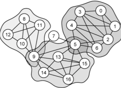
2.14 The overlapping community structure detected by a clique-percolation approach. . 51

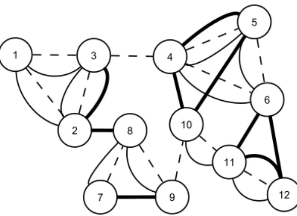
2.15 A multidimensional network. Solid, dashed and tick lines represent edges in three different dimensions. . . 55

2.16 Three graphs generated with the small-world model: (a) p = 0; (b) p = 1 4; (c) p = 1. 61 4.1 An example of layered network (a) and the process of a cascade failure involving the two different layers (b, c and d). In (a) the attacked grey node and its white dependent disappear, with all the edges attached to them, generating (b). Then, the cascade is triggered: the white nodes connected to the disappeared node lose their connections because they cannot sustain them anymore (b→c) and the same happens for the grey nodes (c→d). . . 72

5.1 The friendship dimension in Facebook network. . . 80

5.2 Small extracts of the three real multidimensional networks. . . 82

6.1 A toy example. The solid line is dimension 1, the dashed line is dimension 2. . . . 90

6.2 Cumulative distributions of degree per dimension and global degree for Querylog, Flickr and DBLP-Y. . . 90

7.1 Example of different multidimensional hubs. . . 96

7.2 Toy example and computed measures. Lines: solid = dim 1, dashed = dim 2, dotted = dim 3, dash-dotted = dim 4. . . 99

7.4 The overlap ratio between monodimensional and multidimensional hubs . . . 105

7.5 Some of the multidimensional hubs extracted . . . 105

7.6 The Dimension Correlation computed only between subsequent snapshots (a,c,e) and the corresponding dissimilarities computed on it (b,d,f). We recall that values for the Random and Preferential attachment models are reported but not visible, as they are constant on the 0 line. . . 112

7.7 The Node and Edge Correlation computed among all the snapshots. . . 113

7.8 Eras on both edge and node evolutions in DBLP . . . 114

7.9 Eras in IMDb edge evolution . . . 115

7.10 Eras in IMDb node evolution . . . 116

7.11 Eras on both edge and node evolutions in GTD . . . 121

7.12 Forecasting eras on dissimilarities via autoregressive models . . . 123

7.13 The Node and Edge Correlation in our networks. . . 126

8.1 Three examples of multidimensional communities . . . 130

8.2 Run through example for three instances of MCD Solver varying the φ parameter. 135 8.3 The running times of STEP2 and STEP3 on our networks (color image). . . 136

8.4 The cumulative distributions for γ and ρ in (from left to right): GTD, DBLP-C, DBLP-Y and IMDb datasets. . . 137

8.5 A few interesting communities found, with their γ or ρ. . . 140

8.6 QueryLog (left column) and DBLP-Y (right) original Dimension Relevance distri-butions. . . 141

8.7 Random: QueryLog (left column) and DBLP-Y (right) . . . 142

8.8 Preferential attachment: QueryLog (left column) and DBLP-Y (right column) . . . 143

8.9 Shuffle: QueryLog (left column) and DBLP-Y (right column) . . . 144

8.10 Jaccard: QueryLog (left column) and DBLP-Y (column) . . . 145

8.11 Performances of multidimensional link predictors. . . 147

8.12 A toy example for the multidimensional shortest path with cost modifiers problem. 149 9.1 The Product Space. . . 160

9.2 Community quality for five different ways of grouping products. . . 161

9.3 Contributions to the R square regression over the GDP growth of several different indicators. . . 162

10.1 Data model sketch for Arch¨aologische Bibliographie, including the fat-tail distribtion for classification co-occurrence in publications (upper left, see [232] for detail), and an indication of dataset growth from 1956 to 2011 (upper right). . . 164

10.2 Data preparation, analysis, and visualization pipeline as described in Sections 10.2.1 to 10.2.3, including (a) the one-mode multidimensional projection from publication-classification or author-publication-classification to publication-classification co-occurrence, (b) the creation and visualization of rule-mined directed lift significance link weights in addition to regular co-occurrence weights, and (c) the creation and visualization of the multidi-mensional link community network, using Vespignani-filtering and Hierarchical Link Clustering. . . 165

10.3 (a) Relative number of nodes and edges size for different filtering thresholds. (b) Partition density values for each dendrogram cut threshold for each decade. Higher values means denser partition, i.e. a better community division. . . 167

10.4 Era structure dendrogram of classification cooccurrence in publications of Arch¨aologische Bibliographie according to [40] and Section 7.2. Eras are colored in the tree, while our arbitrary decades are highlighted in the x-axis labels. . . 169

10.5 Communities belonging to various temporal snapshots are connected using a dedi-cated algorithm, revealing interesting merges and splits over time. . . 169

10.6 Links in the community overlap network corresponding to subject themes, locations, and periods are distributed in a very different way. . . 170

10.7 Both classification co-occurrence in publications as well as authors evolve over time, fleshing out structure that emerges early on in the process. . . 172 10.8 Classification co-occurrence (≥ 4) in publications with lift-significance (≥ 0.056) for

the branch Plastic Art and Sculpture. . . 173 10.9 Classification co-occurrence evolution clearly shows that initially highly significant,

i.e. dark links become less significant and wider as they accumulate literature. . . 174 10.10Mutual self-definition of Names Portraits. . . 174 10.11Combining global and meso-level exploration by zooming into overlapping

commu-nities containing a given classification - here Paestum - reveals its meaning even to the uneducated eye, improving significantly over simple ego-networks (see 10.4.2). . 175

2.1 Resume of the main notation used in this section. . . 27

2.2 Resume of the community discovery methods. . . 29

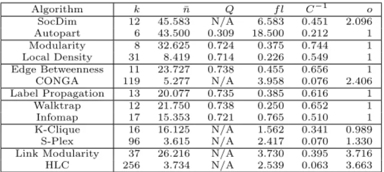
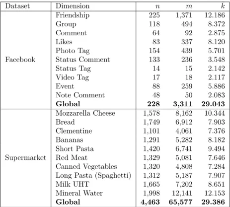
2.3 The evaluation measures for the communities extracted with different approaches. 57 5.1 Main statistics about Facebook and Supermarket networks, and their dimensions. . 81

5.2 Summary of the datasets extracted from Flickr, DBLP and Querylog. Column 1 specifies the dataset; Column 2 the dimension into account; Columns 3 and 4 the number of nodes and edges; Column 5 the average degree; Column 6 the density computed as number of edges out of number of total possible edges in all the dimensions 83 7.1 Relationship between mono and multidimensional hubbiness of a node . . . 103

7.2 Era labels on both DBLP edges and nodes . . . 117

7.3 Era labels on both IMDb edges and nodes . . . 119

7.4 Era labels on both GTD edges and nodes . . . 122

7.5 Dimension Connectivity, HRC, LRC, OCN and OCP of our networks. . . 126

8.1 Number of communities found (|C|) and modularity (Q) for each combination of network and parameters. . . 137

Introduction

A complex network is a model used to represent complex interacting phenomena such as social interactions among human beings, biological reactions in organisms and technological systems. An interaction takes places when there is some sort of information or physical exchange between two actors, for example in a social network when two individuals establish a friendship or enmity link between each other. To analyze the properties and understand the behavior of these phenomena through this model in different settings is a scientific field gaining a lot of attention in the last decade. Countless different problems have been tackled and an impressive number of good solu-tions, algorithms and descriptions of reality, has been proposed. A very brief, and incomplete, list includes the following main topics:

ˆ Community discovery, i.e. the decomposition of a complex network in its modular structure [78, 94];

ˆ Link prediction, i.e. the prediction of the new relations that we will observe given the current state of the network (or the discovery of possible missing connections due to incomplete data) [74, 207];

ˆ Flow analysis, i.e. the analysis of the structural properties of networks unveiled by different random walk strategies over the edges of the graph;

ˆ Cascade events, i.e. the investigation over the dynamics of epidemic events changing the state of nodes through their connections [111];

ˆ Graph motifs mining, i.e. the discovery of regularities in the connection patterns of the nodes in the network [268].

By exploiting the tools developed in the investigation of these topics, and usually combining them with each other or other analytic tools, complex network analysis has been used to tackle many specific problems. For example, link prediction algorithms can be used to predict whether a user will trust the information provided by another user in a recommendation system [170]; or flow analysis is used for web page ranking in the popular Google search engine [208].

How can we explain this amount of interest by the scientific community? First of all, complex networks are by definition complex systems. A complex system is a system composed of different parts that expresses at the global level properties that are not present in any single part taken alone. Their importance is derived by different factors. First, they are ubiquitous: complex systems are present in many different scientific fields such as biology (the brain), ecology (the Earth climate), engineering (telecommunication structures) and many more. Second, to understand what originates their global properties is non trivial and can lead to important scientific results, such as deeper understanding of how the human brain works or a prediction of the evolution of the Earth’s ecosystem.

This makes complex network analysis a suitable test field for many different approaches and theories. In fact, crucial advancements in this field have been carried on by different professional figures: computer scientists, mathematicians, physicists, but also sociologists, economists and humanities scholars. Complex network analysis is a melting pot of different disciplines, where different backgrounds can find a common vocabulary and primitives, making this novel field a truly new branch of science for the next years. Thus, we have a further reason for explaining the success of complex networks: their ubiquity in modeling such different phenomena.

The clash of many different areas of expertise has lead complex network analysis to be applied to many and different problems. Novel problems and settings have been explored in recent years with this model. Clearly, to be useful a model has to represent the features of real world phenomena in a simple way, but without losing too many details in the process. Therefore, from the original simple graph, many extensions have been proposed: weighted, dynamic, asymmetric relations are now fundamental building bricks of any study aiming to unveil novel insights about the interacting phenomena in the real world. However, these extensions do not address a critical feature, present in many interacting phenomena. In fact, weighted or directed relations do not help us when we are dealing with phenomena characterized by multiple different kinds of interactions.

We are not the only researchers that raised this issue. We will see that some intuitions about the intrinsic multifaceted nature of the real world are already present in literature. But it is not necessary to perform experiments or to deeply study obscure data to understand that multiple different relations interact with each other everyday everywhere. Let us consider the case of a social network. At the present day, a person can establish a social relation with hundreds of different people. Are all these people “friends”? Is it possible to organize all these relationships in the same class? Of course not: we have relatives, sentimental relationships, work mates and several different reasons, and degrees, to call the people we know “friends” or “acquaintances”.

To be just a little more formal, it is well known that complex systems show their complexity in their multifaceted dynamics. There are several different competing forces acting either inde-pendently or in a complex interaction, either in equilibrium or in disequilibrium. As for complex networks, the interplay among different relations cannot be expressed with the traditional single relational models. In particular, the simple graph, a simplified representation used in the latter years, is not enough for this increase in complexity.

In this shift of setting and representation, also the traditional complex network analysis needs to evolve and embrace the new complexity it is supposed to explain. If reality is multifaceted, or as we name it in this thesis “multidimensional”, then also network analysis should be multidimensional. Here we introduce the term “dimension” to indicate a particular edge type in a complex network. It is not an equivalent of the term “relations”. While each different relation is a dimension of a network, a dimension may also be a quality of the same relation, such as the different discrete points in time when the relation was present. We will address this distinction more formally in the thesis.

Just as non-linear and non-equilibrium systems needs a new paradigm for statistics, called su-perstatistics, multidimensional networks need new models (multigraphs, data tensors, and so on) and tools (multidimensional community discovery, multilink prediction, shortest path in multi-graphs with cost modifiers, just to name some of them). This is exactly the aim of this thesis: the creation and study of a Multidimensional Network Analysis, to extend the known metaphors of complex network analysis and grasp the complexity of real world phenomena.

In this thesis we want to accomplish several objectives. First, we want to advocate the urgency and need for a multidimensional network analysis. We present an empirical proof of the ubiquity of this multifaceted reality in different complex networks. We are able to create multidimensional representations of many different interacting phenomena. We want also to let emerge the fact that these multidimensional representations are indeed more accurate than a simple monodimensional model, and/or can lead to better insights about the phenomenon being represented. The need for a multidimensional network analysis is also witnessed by many other researchers, and we provide a collection of their early works in this novel analytic setting. We also point out that these applications are indeed useful and advanced, but a common analytic ground, needed to fully understand and develop novel insights, is yet to be defined.

The preliminary steps in the definition and creation of this common ground are exactly the second main objective of this thesis. We want to tackle this problem at two different levels. We start by looking at the basic extensions of the known model: what is the new meaning of the degree in the multidimensional network analysis? What does happen to the scale free structure in a multirelational environment? What is the new relation between the degree and the number of neighbors for a node? How does multidimensionality influence the clustering coefficient or the centrality measures?

We then move our attention to the development of novel algorithms and frameworks for well-understood and useful traditional problems in complex network analysis. For example, we are interested in multidimensional community discovery, that we take as the main case study of this thesis, and therefore tackled with special attention. Traditionally, in community discovery the problem definition is to find a graph partition, clustering together densely connected sets of nodes. If we translate this problem definition in multidimensional terms, we want to find sets of nodes multidimensionally densely connected. But what does “multidimensionally dense” mean here? Does it mean that all the different relations need to be expressed for each couple of nodes? Or that is it necessary that at least one relation is expressed at a time for each couple, and it is only required that different relations connect different couples? This ambiguity will be tackled down in this thesis.

Another example is link prediction. Link prediction has a straightforward problem definition: to rank not observed edges, i.e. couples of nodes, according to how likely they are to appear in the future (or how likely they are not present due to missing data). If we have multiple relations in our network, a new dimension appears. We are not supposed to identify just a couple of nodes that have in between them an unexpected missing link, but we need also to decide in which particular relation, or set of relations. Is it sufficient to simply apply a traditional link predictor to each relation in an independent fashion? Or is it true that actually the different dimensions are influencing each other, and then a completely new framework has to be defined?

As a last example, we want to consider how to include known analysis frameworks into mul-tidimensional network analysis. In fact, we are interested in how a dynamic framework can be included into a multidimensional formulation. If we consider time as source of dimensions, i.e. a relation established in 2012 is a dimension and the same relation in 2011 is another dimension, then with the primitives of multidimensional networks we can perform temporal analysis. This distinction unveils a characteristic of multidimensionality: it is possible to define two different classes of dimensions, the explicit and the implicit dimensions. We will explain the difference later on in the thesis.

We conclude this thesis with a third objective: an example of how useful multidimensional network analysis can be when applied to analytic real world scenarios. We chose two of them. In the first scenario, we present a network analysis approach to international economics, namely the creation and the analysis of the Product Space, i.e. a network map of products connected if they are frequently co-exported by the same countries. From this analysis, an impressive amount of useful knowledge can be extracted, leading to predictions of new products exported by the countries and even their future economic growth. The aim of this first scenario is to indicate where are the parts in which multidimensional network analysis is able to provide analytic improvements over the monodimensional analysis performed. Our second scenario is the analysis of literature and bibliography in the field of classical archaeology. In this scenario we show how natural and useful the choice of a multidimensional network analysis strategy is in a problem traditionally tackled with different techniques.

This thesis is organized as follows. Each of the aforementioned objectives constitutes a main part of the thesis. The first part, Setting the Stage, is devoted to the presentation of the urgency and need for a multidimensional network analysis. We firstly present some aspects of traditional complex network analysis in Chapter 2. Particular attention is devoted to the case of community discovery in Section 2.3, with an extensive study of the state of the art in the field. We will then briefly define in a formal way our model for multidimensional networks in Chapter 3. In Chapter 4 we explore the literature regarding multidimensional network analysis. In Chapter 5 we conclude our exploration about the need of a multidimensional network analysis by presenting many real

world examples of multidimensional networks, that will be analyzed in the following part of the thesis.

The second part, Multidimensional Network Analysis, is the core of this thesis. Here we tackle our second and main objective: the exploration of the various building bricks of multidimensional-ity in complex networks. We start from the bottom, by creating a simple extension mechanism to translate the most basics network measures into multidimensional basics in Chapter 6. We then take a step further in Chapter 7 by defining a collection of novel measures that acquire a meaning only in the multidimensional setting, and are trivially solved in the monodimensional case. Finally, we conclude our main section by proposing also some more advanced analysis in Chapter 8. In Section 8.1 we propose novel evaluation measures and a framework for the discovery of multidi-mensional communities. The other advanced analysis we consider, with a lower resolution, are generative models for multidimensional networks (Section 8.2), multidimensional link prediction (Section 8.3) and the problem of finding the shortest path in a multigraph with cost modifiers (Section 8.4).

The third part, that concludes this thesis, deals with the real world analytical examples we chose: the Product Space creation (Chapter 9) and the analysis of the co-classification network in classical archaeology, in Chapter 10.

Chapter 11 concludes the thesis, by presenting the future research directions opened by this study.

The three parts of this thesis are based on peer reviewed papers published in international conferences. From the first part, the state of the art of complex network and the main definition of the multidimensional netowrk model are inherited from [37]. In the same paper, we introduced also the basic extension to the complex network model (Chapter 6) and the Dimension Connectivity measures (Section 7.3). Dimension Relevance measures (Section 7.1) and multidimensional network null models (Section 8.2) are introduced and studied in [42]. Dimension Correlation and the mapping of temporal analysis with multidimensional networks (Section 7.2) are published in [41, 40, 43]. The community discovery problem in multidimensional complex networks (Section 2.3 for the review and Section 8.1 for the actual algorithm) has been tackled in [78, 36, 39]. The Product Space analysis (Chapter 9) has been published as a book with Harvard University and MIT [128]. Finally, the analysis of publications in Classical Archeology (Chapter 10) has been presented to scholars both from art history and computer science [233].

Network Analysis

In this chapter we present the basic notions of complex network theory. We will start by explaining how a network is represented with a graph, what variants can be defined for this basic representation and what are the basic statistical properties of graphs. We then present in each section one of the main sub branches of complex network analysis in computer science. We start with the main case study of this thesis, namely the community discovery in complex network, with an extensive review of the field. We provide a novel classification of community discovery algorithms, with the aim of presenting where in this branch multidimensional networks can play an important role (and where multidimensionality is already taken into account). The other subsections are shorter and do not provide an exhaustive classification and literature review, outside the scope of this thesis. These sub branches are: network models, link analysis and information propagation. We provide for completeness also a brief overview of problems not directly tackled in the thesis, such as graph mining and privacy concerns in social networks. Where not otherwise specified, we use as basic references the review works presented in [195] and [66], which provide a more complete collection of literature references.

2.1

The Graph Representation

A graph is a mathematical structure used to model pairwise relations between entities from a certain collection. A network is a set of entities with connections among them. The entities are modeled as nodes. Nodes are also called vertices: in this thesis we will use the terms “node” and “vertex” interchangeably as synonyms, while the term “entity” is used to indicate what a node in the graph represents in the real world. The interactions between nodes are represented by the edges.

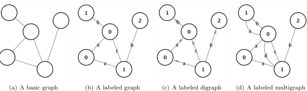
A set of nodes joined by edges, as depicted in Figure 2.1(a), is only the simplest type of network; there are many ways in which networks may be more complex than this. We can add to our representation additional information. Here we present a list of them, taking the example of a classical social network:

ˆ We can add (multiple) labels both to vertices and to edges. Thus, there may be more than one different type of vertex in a network, or more than one different type of edge. For example nodes in a social network can be men or women, or they may have different nationalities, while edges may represent friendship, but they could also represent enmity. An example of labeled graph is depicted in Figure 2.1(b).

ˆ We can add a variety of properties, numerical or otherwise, associated with vertices and edges, thus specifying some attributes. In our social network setting, people can have different ages or incomes, and edges can be weighted by the geographical proximity or by how well two people know each other.

(a) A basic graph (b) A labeled graph (c) A labeled digraph (d) A labeled multigraph

Figure 2.1: Different degrees of complexity in the graph representation.

ˆ Edges can be directed, i.e. they point in only one direction. Graphs composed of directed edges are themselves called directed graphs or sometimes digraphs, for short. A graph repre-senting telephone calls or email messages between individuals would be directed, since each message goes in only one direction. Directed graphs can be either cyclic, meaning they con-tain closed loops of edges, or acyclic meaning they do not. The labeled graph in Figure 2.1(c) has been enriched with the direction on its edges.

ˆ The graph can be bipartite, it means that they contain vertices of two distinct types, with edges running only between unlike types. Examples are the affiliation networks in which people are joined together by common membership of groups.

ˆ Graphs may also evolve over time, with vertices or edges appearing or disappearing, or values defined on those vertices and edges changing.

ˆ One can also have hyperedges, i.e. edges that join more than two vertices together. Graphs containing such edges are called hypergraphs. Hyperedges could be used to indicate family ties in a social network. For example n individuals connected to each other by virtue of belonging to the same immediate family could be represented by an n-edge joining them. ˆ A multigraph is a graph which is permitted to have multiple edges, (also called parallel

edges), that is, edges that have the same end nodes. In Figure 2.1(d) we have represented a very simple labeled multigraph. We have depicted a multigraph with only two double edges, but between the same two nodes there can be an arbitrary number of edges.

All these variants in the graph model enrich the possible representation of real world inter-actions events. In particular it is worth noting that the multigraph model is able to represent multidimensional data. In a multidimensional networks two interacting entities can be connected through different channels. For example in a social network two individuals can connect each other via an instant messaging software, a cellphone call, the membership in a particular website and so on. In Chapter 4 we will see how it is possible to significantly improve the precision and the relevance of a complex network analysis by considering the multidimensional nature of human relationships.

2.2

Statistical Properties

Typical social network studies address issues of centrality (which individuals are best connected to others or have most influence) and connectivity (whether and how individuals are connected to one another through the network). Aim of this section is to present statistical properties, such as path lengths and degree distributions, that are proved to characterize the structure and behavior of networked systems. When possible, we will discuss the meaning and the values taken by a metric on the toy example depicted in Figure 2.2.

Figure 2.2: A network toy example.

The first important notion is the degree. In graph theory, the degree (or valency) of a vertex of a graph is the number of edges incident to the vertex, with loops counted twice. In Figure 2.2 the degree of vertex 0 is equal to 2. Note that the degree is not necessarily equal to the number of vertices adjacent to a vertex, since in a multigraph there may be more than one edge between any two vertices. This is the case of vertex 2 in our example in Figure 2.2. Its degree is equal to 7, while the number of neighbors directly reachable from it is 5. In a directed graph it is necessary to consider also the direction of the edge. Thus each vertex has both an in-degree and an out-degree, which are the numbers of in-coming and out-going edges respectively.

We define pk to be the fraction of vertices in the network that have degree of at least k.

Equivalently, pk is the probability that a vertex chosen uniformly at random has degree k or

higher. A plot of pk for any given network can be formed by making a histogram of the degrees

of vertices. This histogram represents the degree distribution for the network. In a random graph, see Section 2.4.1, each edge is present or absent with equal probability, and hence the degree distribution is Poisson in the limit of large graph size. Real-world networks are mostly found to be very unlike the random graph in their degree distributions. Far from having a Poisson distribution, the degrees of the vertices in most networks are highly right-skewed, meaning that their distribution has a long right tail of values that are far above the mean. These networks are called scale free networks and their degree distributions follow a power law. Scale free networks are proved to be ubiquitous [15].

A network may present a power law degree distribution, i.e. to contain a very high amount of nodes with extremely low degree (1 or 2) and few hubs with a very high degree. There are several explanation for this phenomenon, one of which is the rich-get-richer effect: who has already an high degree have an higher probability of obtaining new edges [30]. This means that in the network there are few nodes with a very high degree and the vast majority of nodes has a very low degree. One statistical parameter that is able to describe how strong is this effect, or in other words how is the ratio between the high degree vertices and the other low degree vertices, is the exponent of the cumulative degree distribution’s slope. In other words the power law degree distribution can be approximate with pk ∼ k−α. This means that the probability that a randomly chosen vertex

has degree greater or equal to k follows this law. It has been experimentally proved that in most of real word networks α takes values between 2 and 3 [195].

The component to which a vertex belongs is the set of vertices that can be reached from it by paths running along edges of the graph. In our toy example in Figure 2.2 we have, for sake of simplicity, only one component. In a directed graph a vertex has both an in-component and an out-component, which are the sets of vertices from which the vertex can be reached and which can be reached from it. In network theory, a giant component is a connected subgraph that contains a majority of the entire graph’s nodes [58]. It has been proved that many real world social networks present a giant component, that collects from 70% to 100% of the nodes of the network. Usually, the Giant Component appears when the average degree is greater than 1 [189].

A geodesic path is the shortest path through the network from one vertex to another. Note that there may be, and often there is, more than one geodesic path between two vertices. In graph theory, the shortest path problem is the problem of finding a path between two vertices (or nodes) such that the sum of the weights of its constituent edges is minimized (or maximized in case the weight of the edge does not represent the cost of going from one node to the other, but the strength of the relation). One can also consider a special case of this problem, in which all edges are unweighted, or their weights are all equal to one. In this case the shortest path is the minimum number of edges to be crossed in order to go from one vertex to another. For example, in Figure 2.2 we do not have weights assigned to our edges. So the shortest path between 0 and 6 pass through node 2, so its length is equal to 2 (2 edges are crossed).

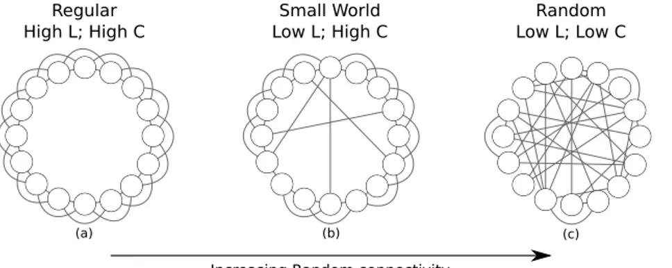
It has been discovered that most pairs of vertices in most networks seem to be connected by a short path through the network. This is the so called small-world effect. In practice, the values of the average length of all the geodesic paths in a network are in many cases quite small, much smaller than the number n of vertices, for instance. It typically increase as log n [262], or even shrink.

The small-world effect has obvious implications for the dynamics of processes taking place on networks. For example, if one considers the spread of information, or indeed anything else, across a network, the small-world effect implies that the spread will be fast on most real world networks. If it takes only six steps for a rumor to spread from any person to any other, for instance, then the rumor will spread much faster than if it takes a hundred steps, or a million. This affects the number of “hops” a packet must make to get from one computer to another on the physical Internet network, the number of legs of a journey for an air or train traveler, the time it takes for a disease to spread throughout a population, and so forth. Many works present in literature take advantage of this knowledge (along with the previously presented power law degree distribution) defining efficient algorithms working with these assumptions. For example, we can use the higher degree nodes in order to optimize the p2p-search task [4].

The diameter of a network is the length (in number of edges) of the longest geodesic path between any two vertices. A few authors have also used this term referring to the average geodesic distance in a graph, although strictly the two quantities are quite distinct. As one can see, the definition of diameter is based on the definition of geodesic path. Thus the value of this metric can change in different models of graph, for example it can be weighted or not. Usually the diameter shrinks in a growing network. This means that if we have a social network and we observe the new users and edges arrival, the distance between the most distant entities usually became smaller and smaller [173]. In the toy example depicted in Figure 2.2, the diameter is equal to 4 (starting from the most isolated vertex 3 to the other side, represented by vertex 7 or vertex 8).

The betweenness centrality of a vertex i is the number of geodesic paths between other vertices that run through i. Some studies have shown that betweenness appears to follow a power law for many networks and propose a classification of networks into two kinds based on the exponent of this power law [107]. Betweenness centrality can also be viewed as a measure of network resilience: it tells us how many geodesic paths will get longer when a vertex is removed from the network. In our example in Figure 2.2 we do not report the entire process needed for computing the betweenness centrality due to the lack of space, but we can give the idea that the vertices 2 and 5 are the most central in the network, because a great part of the shortest paths in the network must pass through them.

Closely related to the betweenness centrality is another centrality index, called closeness centrality. The closeness centrality is the average distance of a vertex from every other vertex in the network. This definition has some known issues when the network has more than one component. As diameter, both betweenness and closeness centrality are defined on the notion of shortest path, thus changing their values depending on the chosen graph model. In literature many other centrality measures are known.

Another important studied phenomenon in real world networks is the transitivity, recorded by the so called clustering coefficient. In many networks it is found that if vertex A is connected to vertex B and vertex B to vertex C, then there is a very high probability that vertex A will also be connected to vertex C. In the language of social networks, the friend of your friend is likely

also to be your friend. In terms of network topology, transitivity means the presence of an high number of triangles in the network, i.e. sets of three vertices each of which is connected to each of the others.

The transitivity property play a crucial role in another studied aspect of complex networks: the community structure, i.e. groups of vertices that have an high density of edges within them and a lower density of edges between groups. In social networks it is straightforward to verify that people do organize themselves into (overlapping) groups along lines of interest, occupation, age, and so forth. This division can be detected in the communities of a network that represents their interactions [190]. Other examples can be citation networks, in which authors would divide into groups representing particular areas of research interest [266]; or in the World Wide Web the community structure might reflect the subject matter of pages.

The detection of this particular structure inside complex networks is one of the most interesting and explored fields of research. We present in Chapter 2.3 some of the most important community detection algorithms, along with their strong points and the open problems. As we will see, also in this research track we are far from getting a definitive answer to the problem of identifying communities in a network. The definition itself of community in a network is controversial, and this stimulated further research.

2.3

Community Discovery

One critical feature of complex networks, which has been widely studied in the literature since its early stages of analysis, is the possibility of identifying groups and communities within the structure of many phenomena represented by this model. Community detection is important for many reasons, such as node classification which entails homogeneous groups, group leaders or crucial group connectors. A “Community” is usually considered to be a set of entities where each entity is closer to the other entities within the community than to the entities outside it. Communities are groups of entities that probably share common properties and/or play similar roles within the interacting phenomenon that is being represented. Communities may correspond to groups of pages of the World Wide Web dealing with related topics [92], to functional modules such as cycles and pathways in metabolic networks [123, 209], to groups of related individuals in social networks [106] and so on.

Community discovery is very similar to the clustering problem, i.e. it is a traditional data mining task. In data mining, clustering is an unsupervised learning task, which aims to assign large sets of data into homogeneous groups (clusters). In fact, community discovery can be viewed as a data mining analysis on graphs: an unsupervised classification of its nodes. In addition, community discovery is the most studied data mining application on social networks. Other applications, such as graph mining [268], are in an early phase of their development. Instead community discovery has achieved a more advanced development with contributions from different fields such as physics. Nevertheless, this is only part of the community discovery problem. In classical data mining clustering, we have data that is not in a relational form. Thus, in this general form, the fact that the entities are nodes connected to each other through edges has not been explored much. Therefore, the concept of spatial proximity needs to be mapped between entities (i.e. vertices) in graph representation.

The traditional and most accepted definition of proximity in a network is based on the topology of its edges. In this case the definition of community is formulated according to the differences in the densities of links in different parts of the network. Many networks have been found to be non-homogeneous, consisting not of an undifferentiated mass of vertices, but of distinct groups. Within these groups there are many edges between vertices, but between groups there are fewer edges. The aim of a community detection algorithm is, in this case, to divide the vertices of a network into some number k of groups, while maximizing the number of edges inside these groups and minimizing the number of edges established between vertices in different groups. These groups are the desired communities of the network.

and of the novel analytical settings, such as the information propagation or multidimensional network analysis. For example, in a temporal evolving setting, two entities can be considered close to each other if they share a common action profile even if they are not directly connected. Thus each novel approach to community discovery has had to face this problem and has developed its own definition of community for its own solution. The underlying definition of community is the criterion that we use to classify community discovery algorithms.

In addition to the variety of different definitions of community, communities have a number of interesting features. These features can be a hierarchical or overlapping configuration of the groups inside the network. Or else the graph can include directed edges, thus giving importance to this direction when considering the relations between entities. The communities can be dynamic, i.e. evolving over time, or multidimensional, i.e. there could be multiple relations and sets of individuals that behave as isolated entities in each relation of the network, thus forming a dense community when considering all the possible relations at the same time. Or they can interact inside all relations, and still the result is a densely connected community, but with a different configuration. We tackle this problem, the ambiguity of the concept of “multidimensional density”, in Section 8.1.

As a result this extreme richness of definitions and features has lead to the publication of an impressive number of excellent solutions to the community discovery problem. It is therefore not surprising that there are a number of review papers describing all these methods, such as [94]. However, existing reviews tend to analyze the different techniques from a very technical perspective. They do not consider organizing the algorithms according to their definition of community, which are many and different as acknowledged also by other papers, such as [200], in which authors say “[all the methods] require us to know what we are looking for in advance before we can decide what to measure”, in which “know what we are looking for” clearly means define what a community is. To use a metaphor, existing reviews talk about bricks and mortar but not about the architectural style. Further, no one considered the problem of community discovery in a multidimensional perspective.

We have thus chosen to cluster the community discovery algorithms by considering their defi-nition of what is a community, which depends on what kinds of groups they aim to extract from the network. For each algorithm we record the characteristics of the output of the method, thus highlighting which sets of features the reviewed algorithm is suitable or not suitable for. We also consider some general frameworks that provide both a community discovery approach and a gen-eral technique. These are applicable to other graph partitioning algorithms by adding new features to these other methods.

We now explain the classification of algorithms based on community definitions. Firstly, we report in Table 2.1 the general notation used in this section. Sometimes we need an additional nota-tion to better explain what an algorithm exactly does. We introduce this addinota-tional notanota-tion when needed and the scope of the additional notation is limited to the paragraph of one particular algo-rithm. Then, before presenting the classification, we make explicit what are the problem features we consider more important for community discovery, including, of course, multidimensionality.

2.3.1

Problem Features

There are many features to be considered in the complex task of detecting communities in graph structures. In this section we present some of the features an analyst may be interested in for discovery network communities. We use them to evaluate the reviewed algorithms in Table 2.2 and also to motivate our classification.

Table 2.2 records the main properties of a community discovery algorithm. These properties can be grouped into two classes. The first class considers the features of the problem representation, the second the characteristics of the approach.

Within the first class of features we group together all the possible variants in the representation of the original real world phenomenon. The most important features we consider are:

Symbol Description

n Number of vertices of the network m Number of edges of the network

k Number of communities of the network ¯

K Avg degree of the network K Max degree in the network T Number of action in the network A Max number of actions for a node D Number of dimensions (if any)

c Number of vertex types (if any) t Number of time step (if any)

Table 2.1: Resume of the main notation used in this section.

(a) Overlapping Communities (b) Directed Community (c) Weighted Communities

Figure 2.3: Different community features.

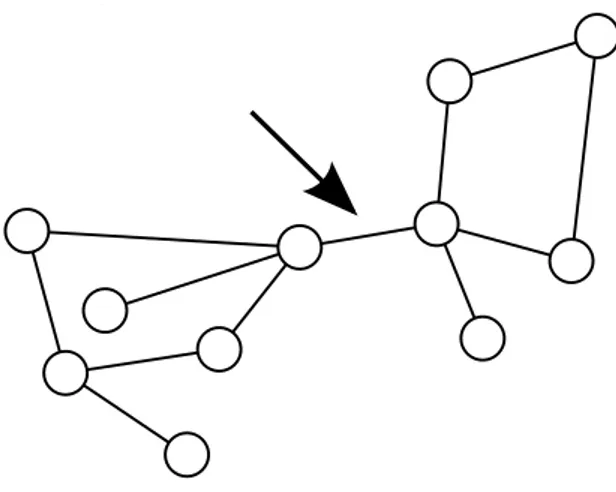
nodes. For example, in social networks actors may be part of different communities: work, family, friends and so on. All these communities will share a common member, and usually more since a work colleague can also be a friend outside the working environment. Figure 2.3(a) shows an example of possible overlapping community partitions: the central node is shared by the two communities. Table 2.2 indicates if an algorithm considers this feature in the “Overlap” column.

ˆ Directed. Some phenomena in the real world must be represented with edges and links that are not reciprocal. This, for example, is the case of the web graph: a hyperlink from one page to another is directed and the other page may not have another hyperlink pointing in the other direction. Figure 2.3(b) shows an example in which the direction of the edges should be considered. The leftmost node is connected to the community, but only in one direction. If reciprocity is an important feature, the leftmost node should be considered outside the depicted community. See “Dir” column in Table 2.2.

ˆ Weighted. A group of connected vertices can be considered as a community only if the weights of their connections are strong enough, i.e. over a given threshold. In the case of Figure 2.3(c), the left group might not be strong enough to form a community. See “Weight” column in Table 2.2.

ˆ Dynamic. Edges that can appear and disappear. Thus, communities might also evolve over time. See “Dyn” column in Table 2.2.

The second class of features collects various desired properties that an approach might have. These features can specify constraints for input data, improve the expressive power of the results or facilitate the community discovery task.

ˆ Parameter free. A desired feature of an algorithm, especially in data mining research, is the absence of parameters. In other words, an algorithm should be able to make explicit the knowledge that is hidden inside the data without needing any further information from the

analyst regarding the data or the problem (for instance the number of communities). See “NoPar” column in Table 2.2.

ˆ Multidimensional input. This is the most important feature in the economy of this thesis. As we already know, multidimensionality in networks is an emerging topic [244, 170, 37]. When dealing with multiple dimensions, the notion of community changes. The concept of multidimensionality is used (with various names: multi-relational, multiplex, and so on) by some approaches as a feature of the input considered by the approach, as we also discussed in Chapter 4. This is the reason why multidimensionality is considered a feature of the input. However, in our opinion, multidimensionality feature should not be placed here, since what we want to extract are truly multidimensional communities. So far, no approach in the community discovery literature is able to do that, and this is the reason why the multidimensionality feature is “misplaced”. We explore the idea of returning multidimensional communities in Section 8.1. See “MDim” column in Table 2.2.

ˆ Incremental. Another desired feature of an algorithm is its ability to provide an output without an exhaustive search of the entire input. An incremental approach to the community discovery is to classify a node in one community by looking only at its neighborhood, or the set of nodes two hops away. Alternatively newcomers are put in one of the previously defined communities without starting the community detection process from the beginning. See “Incr” column in Table 2.2.

ˆ Multipartite input. Many community discovery approaches work even if the network has the particular form of a multipartite graph. The multipartite graph, however, is not entirely a feature of the input that we might want to consider for the output. Many algorithms often use a (usually) bipartite projection of a classical graph in order to apply efficient computations. As in the case of multidimensionality, this is the reason for including the multipartite input as a feature of the approach and not of the output. See “Multip” column in Table 2.2. There is one more “meta feature” that we consider. This is the possibility of applying the considered approach to another community discovery technique by adding new features to the “guest method”. This meta feature will be highlighted with an asterisk next to the algorithm’s name.

Table 2.2 also has a “Complexity” column that gives the time complexity of the methods pre-sented. The two “BES” columns give the Biggest Experiment Size, in terms of nodes (“BESn”) and edges (“BESm”), that are included in the original paper reviewed. Note that the Complexity and BES columns often offer an evaluation of the actual values, since the original work did not provide an explicit and clear analysis of the complexity or their experimental setting. A question mark indicates where evaluating the complexity would not be straightforward, or where no experimental details are provided.

2.3.2

The Definition-based classification

We now review community detection approaches. We group together the algorithms in eight classes sharing the same definition of what a community is, i.e. the same conditions satisfied by a group of entities that allow them to be clustered together in a community. This classification should help to get a higher level view of the universe of graph clustering algorithms, by uncovering a practical and reasoned point of view for those analysts seeking to obtain precise results in their analytical problems. The proposed categories are the following:

ˆ Feature Distance. Here we collect all the community discovery approaches that start from the assumption that a community is composed of entities which ubiquitously share a very precise set of features, with similar values (i.e. defining a distance measure on their features, the entities are all close to each other). A common feature can be an edge or any attribute linked to the entity (in our problem definition: the action). Usually, these approaches propose

Name Ov erlap Dir W eigh t Dyn NoP ar MDim Incr Multip Complexit y BESn BESm Y ear Ref Feature Distance Ev olutionary* X X O (n 2 ) 5k ? 2006 [67] MSN-BD X X O (n 2 ck ) 6k 3M 2006 [179] So cD im X X X O (n 2 log n )∗ 80k 6M 2009 [245] PMM X X O (mn 2 ) 15k 27M 2009 [249] MR GC X X X X O (mD ) 40k ? 2007 [26] Infinite Relational X X O (n 2 c D ) 16 0 ? 2006 [144] Find-T rib es X X O (mnK 2 ) 26k 1 00k 2007 [101] AutoP art X X X O (mk 2 ) 7 5k 500k 2004 [64] Timefall X X X O (mk ) 7.5M 53M 2008 [90] Con text-sp ecific Cluster T ree X X O (mk ) 37k 367k 2008 [211] IntDensity Mo du la ri ty X X X X X X O (mk log n ) 118 M 1B 2004 [75] MetaF ac X X O (mnD ) ? 2M 2009 [178] V a riational Ba y es X X O (mk ) 115 613 2008 [133] LA → I S 2 * X X O (mk + n ) 16k ? 2005 [32] Lo cal Densit y X X X O (nK log n ) 108k 330k 2005 [230] Bridge Edge Bet w eenness X X O (m 2 n ) 271 1k 2002 [106] CONGO* X X O (n log n ) 30k 116 k 2008 [116] L-Shell X X O (n 3 ) 77 254 2005 [22] In tern al-External Degree X O (n 2 log n ) 775k 4.7M 2009 [163] Diffusion Lab el Propa gation X X X O (m + n ) 37 4k 30M 2007 [220] No de Colouring X X O (ntk 2 ) 2k ? 2007 [251] Kirc hhoff X X O (m + n ) 115 613 2004 [267] Comm unic a ti o n Dynamic X X X X O (mnt ) 160k 530k 2008 [108] GuruMine X X O (T An 2 ) 217k 212k 2008 [113] DegreeDiscoun tI C X O (k log n + m ) 37k 230k 2009 [70] MMSB X X O (nk ) 871 2k 2007 [14] Close W alktrap X O (mn 2 ) 1 60k 1.8M 2006 [215] DOCS X ? 325k 1M 2009 [263] Infomap X X X O (m log 2 n ) 6k 6M 2008 [227] Structure K-Clique X O (m ln m 10 ) 20k 127k 2005 [209] S-Plexes En umeration X O (k mn ) ? ? 2009 [155] Bi-Clique X X O (m 2 ) 200k 500k 2008 [168] EA GL E X X X O (3 n 3 ) 16k 31k 2009 [237] Link Link mo dularit y X X X O (2 mk log n ) 20k 127k 2009 [89] HLC* X X X O (n ¯K 2 ) 885k 5.5M 2010 [12] Link Maxim um Lik eliho o d X O (mk ) 4.8M 42M 2011 [25] NoD Hybrid* X X X X O (nk ¯K ) 325k 1.5M 2010 [86] Multi-relational Regression X X ? ? ? 2005 [61] Hierarc hical Ba y es O (n 2 ) 1k 4k 2008 [74] Exp ectation Maximization X ? 1 12 ? 2007 [200]

this community definition in order to apply classical data mining clustering techniques, such as the Minimum Description Length principle [223, 121].

ˆ Internal Density. In this group we consider the most important articles that define com-munity discovery as a process driven by directly detecting the denser areas of the network. ˆ Bridge Detection. This section includes the community discovery approaches based on the

concept that communities are dense parts of the graph among which there are very few edges that can break the network down into pieces if they are removed. These edges are “bridges” and the components of the network resulting from their removal are the desired communities. ˆ Diffusion. Here we include all the approaches to the community discovery task that rely on the idea that communities are groups of nodes that can be influenced by the diffusion of a certain properties or information inside the network. In addition, the community definition can be narrowed down to the groups that are only influenced by the very same set of diffusion sources.

ˆ Closeness. A community can also be defined as a group of entities that can reach each of its own community companions with very few hops on the edges of the graph, while the entities outside the community are significantly farther apart.

ˆ Structure. Another approach to community discovery is to define the community exactly as a very precise and almost immutable structure of edges. Often these structures are defined as a combination of smaller network motifs. The algorithms following this approach define some kinds of structures and then try to find them efficiently inside the graph.

ˆ Link Clustering. This class can be viewed as a projection of the community discovery problem. Instead of clustering the nodes of a network, these approaches state that it is the relation that belongs to a community, not the node. Therefore they cluster the edges of the network and thus the nodes belong to the set of communities of their edges.

ˆ No Definition. There are a number of community discovery frameworks which do not have a basic definition of the characteristic of the community they want to explore. Instead they define various operations and algorithms to combine the results of various community discovery approaches and then use the target method community definition for their results. Alternatively, they let the analyst define his / her own notion of community and search for it in the graph.

In each section we clarify which features in a particular community discovery category of the ones presented in the previous section are derived naturally, and which features are naturally difficult to achieve. We are not formally building an axiomatic approach, such as the one built in [150] for spatial clustering. Instead, we are using the features presented and an experimental setting to make the rationale and the properties of each category in this classification more explicit. The experiments made to support this point are presented after the classification in this section.

Where possible, we also provide a simple graphical example of the definition considered. This example provides a graphical intuition of the main properties of the given classification, in terms of the strong and weak points in particular community features.

The aim of this section is to focus on the most recent approaches and on the more general definitions of community. We are not focusing on historical approaches. Some examples of classical clustering algorithms that have not been extensively reviewed are the Kernighan-Lin algorithm [146] or the classical spectral bisection approach [217]. Thus, for a historical point of view of the community discovery problem, please refer to other review papers.

There is a sort of overlap for some community definitions. For example a definition of internal density may also include communities with sparse external links, i.e. bridges. We see in the Internal Density category that in this definition a key concept is modularity [75]. Modularity is a quality function which considers both the internal density of a community and the absence

of edges between communities. Thus methods based on modularity could be clustered in both categories. However, the underlying definition of modularity focuses on the internal density, which is the reason for the proposed classification. To give another example, a diffusion approach may detect the same communities whose members can reach each other with just a few hops. However this is not always the case: the diffusion approach may also find communities with an arbitrary distance between its members.

Many approaches in the literature do not explicitly define the communities they want to detect or, worse, they generically claim that their aim is to find dense modules of the network. This is not a problem for us, since the underlying community definition can be inferred from a high-level understanding of the approach described in the original paper. One cannot expect researchers to be able to categorize their method before an established categorization has been accepted.

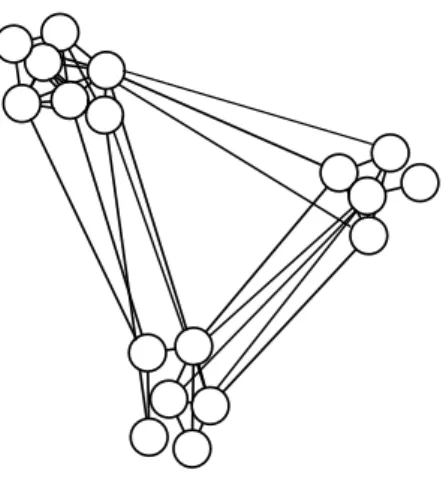
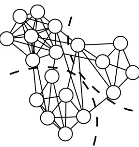
In order to gain stronger evidence of the differences between the proposed categories, consider Figures 2.4, 2.6, 2.8, 2.10, 2.13 and 2.14. These figures depict the simplest typical communities that have been identified from the definitions of Feature Distance, Internal Density, Bride Detection, Diffusion, Closeness and Structure Definition, respectively. As can be seen, there are a number of differences between these examples. The Bridge Detection example (Figure 2.8) is a random graph, thus with no community structure defined for the algorithms in the Internal Density category. The Diffusion example (Figure 2.10) is also a random graph, however although the diffusion process identifies two communities, no clear bridges can be detected.

The overlap is due to the fact that many algorithms work with some general “background” meta definition of community. Further, many algorithms may present common strategies in the exploration of the search space or in evaluating the quality of their partition in order to refine it. Consider for example [161] and [222]. In these two papers there is a thorough theoretical study concerning modularity and its most general form. In [161], for example, the authors were able to derive modularity as a random walk exploration strategy, thus highlighting its overlap with the algorithms clustered here in the “Closeness” category.

Evaluating the overlap and the relationships between the most important community discovery approaches is not simple, and is outside the scope of this section. Here we focus on the connection between an algorithm and its particular definition of community. Thus we can create our useful high-level classification to connect the needs of particular analyses (i.e. the community definitions) to the tools available in the literature. To study how to derive one algorithm in terms of another, thus creating a graph of algorithms and not a classification, is an interesting open issue we leave for future research.

2.3.3

Feature Distance

In this category we review the community discovery methods that define a community according to this meta definition:

Meta Definition 1 (Feature Community) A feature community in a complex network is a set of entities that share a precise set of features (including the edge as a feature). Defining a distance measure based on the values of the features, the entities inside a community are very close to each other, more than the entities outside the community.

This meta definition operates according to the following meta procedure:

Meta Procedure 1 Given a set of entities and their attributes (which may be relations, actions or properties), represent them as a vector of values according to these attributes and thus operate a matrix/spatial clustering on the resulting structure.

Using this definition the task of finding communities is very similar to the classical clustering problem in data mining. In data mining, clustering is an unsupervised learning task. The aim of a clustering algorithm is to assign a large set of data into groups (clusters) so that the data in the same clusters are more similar to each other than any other data in any other cluster. Similarity