S.T.I.T.: asystem of mathematical models for the simulation of land-use and transport interactions

Paper presented at the European Transport Conference 2005, Strasbourg (F) S.T.I.T.: A SYSTEM OF MATHEMATICAL MODELS FOR THE SIMULATION

OF LAND-USE AND TRANSPORT INTERACTIONS

Agostino Nuzzolo, Pierluigi Coppola

Department of Civil Engineering, “Tor Vergata” University of Rome

1 INTRODUCTION

In order to evaluate long-term impacts on travel demand due to changes in transport supply, it is not possible to disregard the effects that such changes have on “land-use” and, indirectly, on travel demand. The problem of simulating such effects has been tackled by different modelling approaches, labelled in literature as “integrated land-use/transport models” (Wilson, 1997).

The term “land-use” covers a variety of topics including urban activities such as residing, and working, the outcomes of market processes such as property or land values, and so on. All these topics can be influenced by changes in transport supply, and may affect travel demand.

In this paper the focus is on the impacts that transport supply has on the distribution of urban activity locations (e.g. residents, services, commerce,…), and, consequentially, on travel demand (e.g. spatial distribution, modal split and so on). Emphasis is given to how zone accessibility impacts on residential and other economic activity and on the competition among urban activities for the acquisition of urban spaces.

The analysis is carried on by means of models dealing with the complex interactions between transportation and urban activities. The range of models proposed to simulate such interactions can be classified in many different ways. Differences can be outlined in the way the system variables are defined, for instance, if space is modelled in a continuous way or in terms of discrete zones, or in the way variables are defined (e.g. endogenously or exogenously with respect to the modelled interactions) and according to different economic theories. Operational modelling approaches are based on the spatial interaction theory (Lowry, 1964) or on the entropy-maximizing theory (Wilson, 1970), in which land use pattern derives from interaction between activities of different zones in analogy with the physical principle of the Newtonian gravity and of the maximum-entropy. Another aggregated approach based on Multi-regional Input/Output model is embedded in the MEPLAN (Echenique, 1990) and TRANUS (de la Barra, 1989) models. The structure of the overall system is based on integrated economic models in which travel demand is the result of interaction between the amount of activities in each zone. Recently, models systems, based upon an explicitly representation of the urban markets (i.e. the labor market, the housing market, the land market and so on) and on the micro-simulation of all the activities processes involved, have been proposed.

Moreover, different approaches stem out of the way in which time dimension is considered. Mainly two different approaches can be distinguished according to the way in which system evolution is studied; in the case of dynamic approach system evolution is explicitly modelled while in the equilibrium or static approach only an internally consistent state of the system is looked for. Key

work in the class of these “pseudo dynamic” models is the model for Dortmund region (Wegener, 1982) and the Delta model (Simmonds, 2000). A comprehensive review of the history of land use-transport interaction modelling is reported in Wilson (1997) and Wegener and Furst (1999).

The paper is organized as follows. In chapter 2, the overall framework of the models system is presented: the travel demand model system and its interactions with the other submodels; the specification of housing and employment location models, calibrated respectively on disaggregate and aggregate data are reported. In chapter 3 an application of the models to the city of Rome (Italy), in order to validate the results of the calibration is finally presented.

2 THE OVERALL MODELLING FRAMEWORK

The system of models presented in the following, can be classified as a spatial interaction model. The overall models system can be cast in a behavioural framework, in which the land use pattern (i.e. housing and activities systems) is the result of the location choices of different decision-makers (i.e. households, firms, …). Interactions between different models are solved through an equilibrium approach. Individual choices of residential and activity location are simulated through Random Utility Theory; the interaction between different individuals (i.e. resident, firms,…) is here simulated through a static (or equilibrium) approach. This approach seems more suitable for practical applications since equilibrium models are easier to be calibrated and implemented, with respect to more complex dynamic modelling framework.

The overall framework, consists of three integrated submodels:

• the Travel Demand submodel, which, given the land-use pattern and the level of service of transportation system, simulates individual travel choices (such as tour frequency, trip distribution and mode choice) allowing to estimate the generalized travel cost and zonal accessibility; • the Residential Location module which, given the generalized travel cost,

the economic activities pattern and the housing supply, simulates the residential location choice of each worker of the study area;

• the Activity Location module which, given the accessibility of each zone and the residential location pattern estimates the amount of socioeconomic activities located in each zone.

Several interactions do exist between different submodels (see figure 1). In facts, travel demand derives from where people leave and where they need or desire to go for different purposes (e.g. workplace, shopping, leisure,…), so it is strictly dependent on the housing and activities distribution within the study area. Travel demand furthermore induces network performances in case of congested networks and, therefore, determines indirectly zonal accessibility. On the other hand, it is reasonable to assume that zonal accessibility influences activities location since the more accessible a zone is to households or to workers the more it is reachable by potential clients (i.e. the households and workers themselves). As consequence, the activity location is linked to both travel demand and residential location submodels.

Figure 1: the overall framework of the models system

Residents/ worker

ratios per zone

Total number of workplaces in Services Total number of workplaces in Commerce O-D matrices by mode and purpose Level of service DEMAND MODELS level, spatial-distribution, modal split ASSIGNMENT MODEL Supply Networks Zonal Accessibility Model Input data Output data Nr. of workers per zone Residents Location Model Workers per zone Houses occupancy rates Services Location model Commerce

Location model Workers in Comm. _{per zone} Workers in Services per zone Mode choice satisfaction Residential Surfaces N. of houses Zonal characteristics Residents per zone Workers in basic activities per zone

Activities occupation

Moreover, since it is plausible to assume that people, ceteris paribus, find more convenient living in zones “closer” to workplace and/or to services and leisure activities, it results that also housing location in turn depends on activities location and on the accessibility to such activities.

As it can be seen, there is a circular dependency between travel demand, residential location and activities location which give rise to a fixed-point problem (Cascetta, 2001). The properties and the algorithms for the solution of such problem are discussed in par. 3.4.

2.1 The transport model

For sake of brevity, in this paper the transport models, which is a traditional four-stages demand model integrated with an equilibrium assignment to road network and to an optimal strategies assignment model to transit network (STA, 1999) will not be described, but only the variables affecting location choices (i.e generalised transportation cost and zonal accessibility) will be pointed out. The origin-destination impedance function is here calculated through the

satisfaction variable (Cascetta, 2001) of mode choices. Accessibility, on the

other hand, is made up of two functions, one representing the activities or the opportunity to be reached for a given purpose and one representing the effort (e.g. time, cost, distance, etc) needed to reach them. We here consider two type of accessibility referred to as “active” and “passive” accessibility.The active accessibility of zone o is a proxy of the opportunity of reaching the activities located in different zones of the study area for a given purpose (e.g. shopping, workplace, …) moving from o. For instance, we can calculate the active accessibility of zone o to the services of the study area, as:

(

)

∑

=

d serv Other

act _{o E d exp Y (o,d)}

A _{( ) ( )}α1 α₂

where Eserv(d) is the number of people employed in services (e.g. banks,

insurance institutes, etc) of zone d; YOther(o,d) is the inclusive values of the

mode choice for “Other purposes” (i.e. shopping, personal care, etc); α1 and α2

are calibrated parameters.

On the other hand, the passive accessibility is a proxy of the opportunity of an activity located in a given zone d to be reached from the potential consumers moving from all the various zones of the study area for a given purpose. For instance the passive accessibility of zone d with respect to households (or equivalently to the whole population of the study area) can be calculated as:

(

)

∑

where R(o) is the number of people leaving (i.e. residents) in zone o; γ1 andγ2

are calibrated parameters.

It is worth noting that variations of network performances (i.e. variations in the generalised travel cost and in the accessibility of the zones) induce variations in housing and activity location (i.e. land use pattern). The land use modification impacts the structure of the demand and, in case of congested networks, can

modify in turn the performance of the transport supply. Thus, there is a circular dependency between network performances and activity location which can be seen as an equilibrium problem or, from a mathematical perspective, as a fixed-point problem (Cascetta, 2001). The analysis of such a mutual dependency is a current issue of research and is out of the scope of this paper. Here we focus on other two equilibrium problems, concerning the location of residents and economic activities, which will be discussed in the following sections.

2.2 The Residential Location Model

The residential location model gives the number of residents in each zone of the study area as a function of the location advantages and characteristics of the supply transportation system. Following a behavioural approach, it is assumed that the choice of the residential zone is the result of the decision-making process of workers present in the study area. Thus, each worker chooses his/her residence zone according to the characteristics of the zone itself (price per square meters, services, etc.), but mainly according to his/her workplace. The probability that each worker i chooses zone o as residential one, Pi_{res(o), is} given by: ∑ ⋅ = d i work i cond -res i res(o) P (o|d) P (d) P where:

- Pires-cond(o|d) is the probability that worker i chooses to live in zone o

conditional to working in zone d;

- Piwork(d) is the probability that worker i is employed in zone d.

It is assumed that the labour market is saturated. Therefore the probability

Piwork(d) is simply given by the ratio between the employed of type i in a given

zone Empitot(d) and the total number of employed of the same type present in

the study area EMPitot:

i tot i tot i work(d) Emp (d) EMP P =

In order to estimate the conditional probability Pires-cond(o|d), consistently with

Random Utility theory it is assumed that each worker i, in choosing his/her residential zone, associates an utility, Uio|d, to all the available zones and

chooses the one which maximises the utility. Uio|d is assumed to be a random

variable consisting of two terms: the systematic utility Vio|d and the random

residual ε_{i. If random residuals} ε_{i are independently and identically Gumble} (0,1)-distributed, the conditional probability Pires-cond(o|d) is given by the

well-known Logit formulation:

∑

-res o|d exp[V o|d exp[ V o'|d

The systematic utility of locating a residence in zone o, given the workplace in zone d, is a function of the following attributes:

• transportation system performances, obtained as the inclusive value of mode choice between o-d pair for “Workplace” purpose and for users of type

i,Yiwork(o,d);

• attributes of the attractiveness of a residential zone o like the logarithm of the number of available houses, LnHouses(o), the price of houses in zone o, expressed in thousands of Euro per square meters, Price(o), and the occupancy rate of houses in zone o, x(o);

• socio-economic attributes of the zone like the indicator of the quality of the estate of zone o, IACP(o), an index of prestige of the zone, Pres(o), as well as dummies dealing with the characteristics of the area to which each zone belongs, i.e. presence of green, panorama, etc.

In order to point out that income may influence residential location choice, residents of the study area have been disaggregated into two socio-economic categories, identified according to the income as it is reported in table 1.The parameters estimation of each attribute present in the model has been carried out through a survey employed in Rome. The method used is that of Maximum Likelihood relative to a zoning of 463 zones of the urban area of the city of Rome. The results obtained are reported in table 1.

Table 1– Parameters (and relative t-ratios) of the residential location model

Yiwork(o,d) Intra(o,d) Price(o) x(o) LnHouses(o) IACP(o) Pres(o)

High 0.476 (6.9) - - -0.536 (-3.1) 0.246 (11.2) -0.639 (-1.7) 0.196 (1.9) Medium/ Low 0.482 (11.8) 0.736 (4.8) -0.716 (-6.6) -0.231 (-4.7) 0.297 (27.7) -0.335 (-1.9) -

It can be noted that the sign of the estimated coefficients is consistent with the behavioural assumptions at the basis of the model, e.g. the coefficient of the

Ln-Houses attribute is positive while that relative to the price Price is negative.

The coefficient relative to the inclusive value of the mode choice, Yiwork(o,d), is

almost the same for the two categories considered. However, the dummy variable Intra(o,d), equal to 1 if the residential zone o and the employment one

d coincide, is positive and significant only for low income workers. This means

that the distance from the workplace zone is a factor affecting residential location choice for low income workers more than for high income ones. This is mainly due to the more flexible working-time of the former, which imply work trips not necessarily in the peak period, when the transportation system is usually congested.

The houses occupancy rate function is given by the following expression:

α ⎟⎟ ⎠ ⎞ ⎜⎜ ⎝ ⎛ = ) o ( sq ) o ( Res ) o ( x

where Res(o) and sq(o) are respectively the residents and the square meters of houses available in zone o, and the constant α, calibrated together with the other model parameters, is equal to 1.88. The coefficient of x(o) is almost double for high income workers compared to the one for low income ones. The attribute Price(o) is not significant for high income categories, while Pres(o) is not significant for low income ones. This points out the different residential location choice behaviour, which justify the introduced workers categorisation.

The equilibrium problem in the residential location

The probability that the generic worker i chooses zone o as a residence zone multiplied by the total number of workers of the study area, Wi , gives the number of workers i in each zone o, wi(o).

It follows: i i res i W o P (o) w = ( )⋅

or equivalently, under the assumption that the total number of workers i is equal to the number of employed of the same category, EMPi=Wi , it results:

∑

Given the number of workers for each zone of the study area, it is possible to get the number of residents in the same area through a coefficient k(o), which represents the ratio between residents and workers in zone o:

∑ ∑ ⋅ ⋅ = i d i i cond -res (o|d) Emp (d) P ) o ( k ) o ( Res

From the previous section, it is deduced that the probability of living in a zone conditional to the workplace, Pires-cond(o| d), depends on a set of attributes,

among them the occupancy rate of houses in zone o, x(o). The latter depends itself on the number of residents of the zone. Therefore, let Ri be the [n_zone x 1]-vector of residents of type i, Ai the [n_zone x 1]-vector of the total employed of type i, x the [n_zone x 1]-vector of occupancy rates of the zones of the study area, ki the [n_zone x 1]-vector of the ratios between the workers and residents of type i, Pi the [n_zone x n_zone]- matrix of the residential conditional probabilities relative to workers of type i, it follows:

(

)

∑

Therefore, there is a circular dependency among residents, occupancy rates and houses availability. This can be treated as a fixed-point problem, whose solution is represented by vectors Ri* and x*:

(

)

∑

The existence of the equilibrium solution is proved by the fact that the possible solutions set Ri and the occupancy rate function follow the conditions imposed by the Brouwers’ theorem (Cascetta, 2001). The uniqueness of the solution is given by the fact that the function x(⋅) is strictly monotone and the residential

choice model is additive.

2.3 The Economic Activity Location Model

The economic activity location model allows to determine the distribution of the number of employed in the economic sectors a, Empa(d), in the single zones d

of the study area through the estimate of the probabilities, Pa(d), of locating an

activity of sector a (e.g. retail, wholesale, etc.) in a given zone d. Be EMPa the

total number of employed in the economic sector a of the study area, it follows:

a a

a(d) P(d) EMP

mp

E = ⋅

In the model under analysis, activities are grouped in the following economic sectors:

• Basic activities (e.g. Public Administration, Welfare, University, …)

• Demand-oriented activities (e.g. retail commerce, services to families,…) • “Representative” activities (e.g. central administration of Banks )

• “Low-spatial efficiency” activities (e.g. wholesale commerce).

Basic activities are those activities whose location is exogenous with respect to

transportation system (e.g. location of industries, universities, etc.) but depends on strategic planning actions. Demand-oriented activities are those activities

whose location depends on residents distribution over the study area and on zonal accessibility Representative activities are those oriented to zones which

have intrinsic attractiveness such central or prestigious ones, while the Low-spatial efficiency are those which requires great spaces such us car sellers,

furniture retailer and so on. In the following the focus is on demand-oriented activities locations; other activities location is considered as input data. In particular, we focus on two types of demand-oriented activities location choice (i.e. Private Services and Commerce). To simulate these location choices a behavioural approach consistent with Random Utility theory is followed. Private investors (i.e. firms, craftsmen, companies, etc.) in choosing the zone d where

to locate their activity, associates an utility, Uad, to all the available zones and

chooses the one which maximises Ua(d). Utility is assumed to be a random

variable consisting of two terms: the systematic utility Va(d) and the random

residual ε_{a. If random residuals} ε_{i are independently and identically Gumble} (0,1)-distributed, the probability Pa(d) of locating activity a in zone d, is given by

∑

The systematic utility Va(d) is a linear combination of the attributes taking into

account:

• transportation system performances, i.e. accessibility (active and passive) of the zone;

• attributes of the attractiveness of the zone, like the number of residents and the number of employed in the basic sector present in the same zone;

• dummies taking into account the characteristics of the area to which a given zone belongs, like Centre, which is equal to 1 if the zone is central 0

otherwise.

Two different activity location models have been calibrated: one for the services and one for the commerce. The calibration has been carried out on Census data of the urban area of the city of Rome. The calibration results are reported in table 2.

Table 2. employment location model parameters (t-ratio between brackets).

Accpas Res(d) Empbasic Centre

Services 0.137 (3.6) 0.011 (2.8) - 1.585 (3.0) Commerce 0.105 (1.9) 0.075 (2.6) 0.049 (2.4) 1.397 (2.1)

Passive accessibility has the expression reported in section 3.1; in this case the constant γ1 and γ2, calibrated together with the other model parameters, are

equal to 0.85 and 1.22 respectively.

All the estimates are statistically different from zero and have the expected sign. As it can be noted, the parameters β_Accpas are positive meaning that the more

accessible a zone is to residents the more it is convenient to locate there an activity. While the values of β’s relative to accessibility are comparable for

“Services” and “Commerce”, this is not true for those relative to population. The

βRes is almost seven times bigger for “commerce” than for “Services”, as if the

distribution of commercial activity resembles very closely the distribution of population among the zones. Furthermore, basic sector activities of the zone are not significant for “Services” sector. Finally, location in a central area is very convenient both for services and commercial activities due to the historical and social factors typical of such area.

2.4 The Equilibrium Problem between Economic Activities and Residence Location

Given the number of employed in each economic sector a and zone d, Empa(d),

it is possible to get the number of employed in zone d of type i, Empi(d), as:

∑

where hia(d) represents the rate of workers of type i employed in an activity of

the sector a in zone d.

From the assumptions on the residence location, it follows that the number of residents of type i in a given zone depends on the distribution of the employed.

Viceversa, the number of employed (of the same type) in a given zone depends on the number of residents in the same zone. Therefore, let Ai be the [n_zone x

1]-vector of employed of type i in a given zone, it follows:

[

]

[

]

∑

∑

Therefore, an equilibrium problem exists in the activity and residential locations, whose solution is given by the vectors Ri* and Ai*:

[

]

[

]

∑

∑

The existence of the vectors Ri* and Ai* is once again proved by the conditions

of the Brouwers’ theorem.

3 THE APPLICATION OF THE MODEL TO THE CITY OF ROME

In order to evaluate the results of the estimation phase, the system of models have been applied to the city of Rome. The whole population of the study area is over 2,7 million and total number of worker is about 950,000. The model has been applied to the more detailed zoning, consisting of 463 zones, however the results are shown for the aggregate 54 macro-zones. The equilibrium problem (8) has been solved using the MSA algorithm. The results of the application of the models system are very promising and show the way for further improvements.

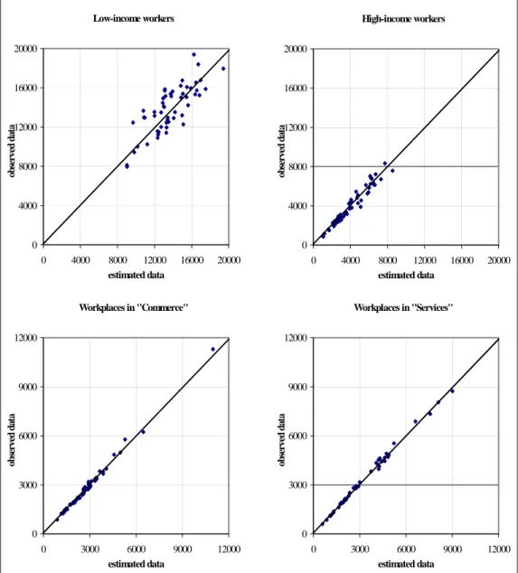
Low-income workers 0 4000 8000 12000 16000 20000 0 4000 8000 12000 16000 20000 estimated data ob serv ed da ta High-income workers 0 4000 8000 12000 16000 20000 0 4000 8000 12000 16000 20000 estimated data ob se rve d d at a Workplaces in "Commerce" 0 3000 6000 9000 12000 0 3000 6000 9000 12000 estimated data ob se rve d d at a Workplaces in "Services" 0 3000 6000 9000 12000 0 3000 6000 9000 12000 estimated data ob se rve d d at a

Figure 2: housing and employement location: observed vs. estimated data. Concerning housing location, the percentage error between observed and estimated workers for the 54 macro-zones ranges from -8% to +8% with peaks of 20 % for few more aggregated suburban ones. The scatter diagrams, depicted in figure 2, show a bigger dispersion for low income than for high-income workers: a more disaggregate segmentation of low income could probably better off the estimates. Concerning employment location, the percentage error between macro-zones ranges from –4% to +4%, no peaks are observed as in the case of housing location, as shown in figure 2.

Once validated, the model system has been applied to the study area in order to evaluate the effects of changes in the transport supply configuration. The analysis of the impacts of such changes has been carried out in terms of changes in housing and activity locations as well as in demand flows (e.g. zonal emission/attraction, modal split). In this respect, a comparison with the estimates carried out by traditional four-stages demand models, is presented.

Table 3: residents and employees for each “macro-zone”. Workers Residents (>14 y.o.) Employed in commerce Employed in services Employed in basic sectors Centre 16.052 45.347 18.019 42.990 63.971 Ring 1 159.745 430.012 39.941 145.238 161.866 Ring 2 381.082 968.927 60.789 69.698 137.508 Ring 3 412.729 961.864 46.927 55.954 112.870 total 969,608 2,406,150 165,676 313,880 476,215

The typical case of the introduction of Travel Demand Management (TDM) policies in the highly congested zones of the city centre, has firstly been analysed. In doing so, the study area has been split into four different “macro-area ”: the “Centre” consisting of the historical centre of the city and three concentric circular sector, namely the “ring 1”, the “ring 2” and the “ring 3”.

In table 3 the number of residents and of employed for different sector is reported for each macro-zone.

With respect to a reference scenario in which only the zone of the “Centre” are already subject to TDM policies (i.e. parking fares and access limited only to residents), the extension of parking fares to all the zones of the ring 2 has been simulated. The result of this first run of simulation are reported in table 4, in terms of percentage variation of the number of residents, employed in commerce and employed in services.

Table 4: percentage variation of residents and employed due to the introduction of parking fare in the sub-central zone

Workers Employed in commerce Employed in services

Centre 482 3% 3.439 8% 7.677 12%

Ring 1 14.377 9% -7.262 -5% -17.805 -11%

Ring 2 -10.670 -3% 2.788 4% 6.875 5%

Figure 3 - Housing percentage variation within the study area due to new underground railways (depicted with blue lines).

Figure 4 – Services percentage variation within the study area due to new underground railways (depicted with blue lines).

< -15% -15% - -2% -2% - 2% 2% - 15% > 15% Variazione percentuale della poplazione < -15% -15% - -2% -2% - 2% 2% - 15% > 15% Variazione percentuale degli addetti ai servizi privati

As it can be seen, for a given zone o, the introduction of parking fares induces an increasing number of residents and a decreasing number of activities such as services and commerce. This can be explained that the parking fares increases the generalised travel cost towards the zone o and determines a reduction of the passive accessibility of this zone. Therefore, people working in o (i.e. the zones subject to new parking fares) tend to move residence towards these zones to minimise the effect of the increased generalised travel cost to their workplaces. On the other hand, consultants, banks and other private investors tend to locate their activity in other zones which results more attractive for potential clients, having an higher (passive) accessibility.

The introduction of a new underground railway and the extension of existing ones have then been simulated. The results in terms of variation in housing and economic activities location are depicted in figures 3 and 4. It can be observed that the effects of the changes in the transport supply system in this case, induce an increasing number of both housing and economic activities in the zone served by the new Public Transport infrastructure. This increasing on the average is between 5% and 15% and is higher in the peripheral zones, where the marginal increase of accessibility is higher.

In terms of demand flows it can be observed an increasing of 24.9% of the trips generated by the zones served by the new underground railway and of 8.0% of the trips attracted. Table 5 shows that the same indicators are underestimated using traditional four-stages demand models.

Table 5: percentage variation of trip on Public Transport modes generated and attracted by zone served by the new Public Transport infrastructure.

Land-use/transport interaction model Traditional four-stages demand model Trip generated 24.9% 19.5% Trip attracted 8.0% 1.6%

Finally, in terms of modal splits table 6 shows the modal shares in a scenario with the introduction of TDM policies and of the new Public Transport infrastructures, estimated by means of four-stages demand models and the adopted modelling framework. Also in this case the estimates obtained by mend of traditional four-stages models seems to underestimates the impacts of the simulated transport changes.

Table 6: modal shares using different models in case of new Public Transport infrastructure and TDM policies.

Private modes share Public transport share Reference scenario 63.6% 36.4% Traditional four-stages

demand model estimates 58.3% 41.7%

New underground railway

and TDM policies land-use/transport

4 CONCLUSIONS

In this paper a system of spatial interaction models aiming at simulating land-use and transport interaction is presented. The overall framework consists of integrated behavioural submodels in which land-use pattern derives from the location choices of different decision-makers (i.e. households, workers, firms, companies, etc). Preliminary version of the models system, though fully operational, is characterised by an aggregate definition of economic sectors and worker typology. This leads to estimates values which, however promising, could be easily better off by further segmentation. Calibration of further attributes (e.g. accessibility to services in the housing location submodels, prices of commercial surfaces in the commerce submodels, etc.) to include in the utility functions could be tested as well. Interactions between different submodels (i.e. different components of the urban system) are simulated through an equilibrium approach. Conditions for existence and uniqueness of the equilibrium solution are discussed. Although preliminary applications of the models system show a fast convergence to an equilibrium solution, the properties of convergence of the adopted algorithms needs to be investigated more deeply.

Applications to the urban area of Rome (Italy) showed a reasonable elasticity of housing and activity location with respect to changes in transportation supply pattern induced by TDM policies and/or new infrastructures. This allows improving the estimates of demand flow obtained using traditional demand models.

BIBLIOGRAPHY

Cascetta, E. (2001) Transportation Systems Engineering: theory and methods,

Kluwer, MA.

De la Barra T. (1989) Integrated Land-use and transport modeling. Cambridge

University Press.

Echenique M. et al. (1990) The MEPLAN model of Bilbao, Leeds and Dortmund. Transport Review, 10, pp. 309-322.

Lowry I. S. (1964) A model of Metropolis. RM-4125-RC, The Rand Corporation, Santa Monica (California).

Simmonds, D. C. (2000) The objectives and design of a new land-use modelling package: DELTA, Report of the David Simmonds Consultancy.

STA (1999) .Un sistema di modelli di domanda per la simulazione della domanda di mobilità nell’area urbana di Roma. Internal report, Rome.

Wegener, M., and Furst, F. (1999) Land-use and transport interaction: state-of-the-art, project funded by the European commission under the transport RTD programme of the 4th framework programme.

Wegener M. A (1982) Multilevel Economic Demographic Model for the Dortmund Region. Sistemi Urbani, 4, pp. 371-401.

Wilson, A.G. (1997) Land use/transport interaction models - past and future.

Journal of Transport Economics and Policy, 32, 3-23.