Study of aerosol scavenging processes in atmosphere

(1)

(2)

(3)

List of Figures

1.1 Size range of particles in the atmosphere . . . 9

1.2 Number distributions of tropospheric particles . . . 10

1.3 Film droplets and jet drops . . . 12

1.4 Aerosol Optical Depth . . . 20

1.5 Changes in cloud microstructure due to aerosols . . . 21

1.6 Aerosol removal . . . 24

2.1 The droptower scheme . . . 30

2.2 vthr as a function of the Kn number. (Experimental data) . . 34

2.3 The pressurized capsule of the Bremen drop tower . . . 36

2.4 An example of cell used for experiments . . . 37

2.5 Monodisperse aerosol generator (Mage) . . . 39

2.6 vs versus Kn number (Ar, Xe, and N2 as carrier gas) . . . 41

2.7 vs versus Kn number (He as carrier gas) . . . 42

2.8 Experimental data and Waldmann’s solution for vs . . . 43

2.9 Experimental data compared with the data of Schmitt and Jacobsen and Brock . . . 45

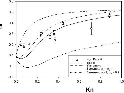
2.10 Comparison of theoretical models with the experimental re-duced thermophoretic velocity (N2 as carrier gas). . . 46

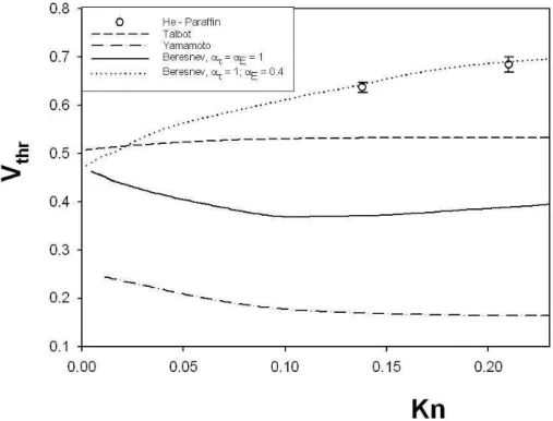
2.11 Comparison of theoretical models with the experimental re-duced thermophoretic velocity (He as carrier gas). . . 47

2.12 Comparison of theoretical models with the experimental vthr (Ar as carrier gas) . . . 48

2.13 Comparison of theoretical models with the experimental vthr(Xe as carrier gas). . . 49

3.1 The Gibbs free energies . . . 55

(6)

3.3 Time series of CCN concentration (cm−3_{). . . .} ₆₂

3.4 Trend of CCN concentration and relative humidity (S=0.36%). 62 3.5 Trend of CCN concentration and mixing layer height (S=0.36%). 63 3.6 Time series of aerosol number concentration (range 0.3-1µm, l−1_{) and CCN (cm}−3_{). . . .} ₆₄

3.7 CCN concentrations in published papers. . . 66

3.8 Ratio CCN/CN; S=0.36%. . . 67

4.1 Wind rose at San Pietro Capofiume . . . 75

4.2 The schematics of the chamber. . . 76

4.3 Ice crystals and blank filter . . . 78

4.4 Time series of concentrations of IN(Tair = -15 ◦C, Tf ilter = -17◦_C) _{. . . .} ₇₉

4.5 Time series of concentrations of IN (Tair = -15 ◦C,Tf ilter = -18◦_C) _{. . . .} ₈₀

4.6 Time series of concentrations of IN (m−_{3) active at T} air = -17◦_{C, T} f ilter = -19◦C. . . 80

4.7 Time series of concentrations of IN (Tair = -15 ◦C; Sw = 2% and Sw = 10%. . . 82

4.8 IN concentration (m−3_{) in TSP averaged over two wind} sec-tors. . . 83

4.9 Time series of particle concentration measured with optical (l−1_{) and CN counters (cm}−3_{). . . .} ₈₃

4.10 Correlation between IN in total suspended aerosol and CN concentration. . . 84

4.11 Map of Po Valley showing the observation site . . . 86

4.12 Time series of concentrations of IN (m−3 _{) active T} air = -15 ◦_{C; T} ice = -17 ◦C (Sice= 20%; Sw = 2%). . . 88

4.13 Time series of concentrations of IN (m−3 _{) active T}_air _{= -15} ◦_{C; T} ice = -18 ◦C (Sice= 32%; Sw = 10%). . . 89

4.14 Time series of concentrations of IN (m−3 _{) active T}_air _{= -17} ◦_{C; T} ice = -20 ◦C (Sice= 34%; Sw = 9.6%). . . 89

4.15 Wind rose of 7-8-9-10 February. . . 90

4.16 Mean value of IN concentration vs. Sice and Sw . . . 91

4.17 Mean concentration of IN concentration at Tf ilter = -18, -19, -20◦_{C, T}_air _{= -17}◦_{C (P M} 10 fraction). . . 91

(7)

4.18 Correlation between IN concentration (m−3_{) measured at (T} air

= -17 ◦ _{C; T}_{f ilter} _{= -20} ◦_{C) in total suspended aerosol and}

aerosol concentration, d > 0.3µm(m−3_{). . . .} ₉₂

5.1 DustTrak, TSI . . . 97

5.2 Measurements of P M2.5 indoor . . . 98

5.3 Measurements of P M2.5 indoor . . . 98

5.4 Scatter plot between r.h and concentration . . . 100

5.5 Scatter plot between r.h and concentration (r.h > 80%) . . . 100

5.6 P M2.5 concentration(June 16, 2010) . . . 101

5.7 Output of Pludix (June 20, 2010) . . . 102

5.8 P M2.5 concentration (June 20, 2010) . . . 102

(8)

INTRODUCTION

The study of aerosol is interesting for a number of reasons: direct (scat-ters and absorbs solar and infrared radiation) and indirect effects (modifies microphysics of clouds serving as condensation nuclei and ice nuclei) on cli-mate, effects on human health and ecological hazard, just to mention some. In recent decades it is worth taking into consideration two events in which the concentration of aerosol influenced the climate. In 1991, the vio-lent eruption of the volcano Pinatubo has scattered 15 million to 30 million tons of sulfur dioxide in the atmosphere, causing a decrease in average global temperature of the planet within two years. In 2001, the interruption of air traffic in North America, following the attack on the Twin Towers in New York, coincided with an increase in daytime temperature (∼ 1 ◦_{C). This}

shows that the effect of the reduction of aerosol and contrails of the aircraft was to increase the incoming solar radiation on the Earth’s surface. Aerosol concentrations and forcing will change in the future, as a result of changing emissions, related to the growth of the population. The uncertainties associ-ated with our knowledge of the present day distribution of aerosols will have consequences to the analysis of future scenarios. Seen in context, a better understanding of the scavenging of aerosol in the atmosphere is of crucial importance.

The aim of this thesis is to increase the knowledge of aerosol removal through processes linked to clouds (thermophoresis, ice nuclei, cloud con-densation nuclei and impaction scavenging), by means of experimental stud-ies.

Thermophoresis describes a phenomenon in which particles suspended

in a fluid with no uniform temperature are subject to a force, named ther-mophoretic force, which is counteracted by the fluid drag on the particle. Thermophoresis plays a role in the scavenging of aerosol particles in clouds.

(9)

This process happen in cloud because during processes like condensation or evaporation, temperature gradients are formed in clouds. In normal gravity it is not possible to study the phoretic effect alone, as particles move due to gravity and due to natural convection resulting from temperature gradi-ents established to study thermophoresis. So experimgradi-ents were performed in microgravity conditions. Concerning the study of the thermophoresis I carried out preliminary studies in normal gravity regarding aerosol genera-tion and characterizagenera-tion and many experiments to test the apparatus for the microgravity campaigns. Measurements of the thermophoretic veloci-ties of aerosol particles in different carrier gases (helium, nitrogen, argon, xenon) were performed in microgravity conditions (the drop tower facil-ity, in Bremen). The experiments permitted the study of thermophoresis in conditions which minimize the impact of gravity. Particle trajectories, and consequently particle velocities, were reconstructed by analyzing the sequence of particle positions.

Cloud condensation nuclei are atmospheric aerosol that serves as

parti-cle upon which water vapor condenses to form droplets that are activated and grow by condensation to form cloud droplets at the supersaturations achieved in clouds. As to this study, I helped in the realization of the ther-mal diffusion chamber, used in the experimental campaign performed in S. Pietro Capofiume (in which I took part). Then experiments to test the chamber and the acquisition system were carried out. Subsequently we ana-lyzed data correlating them with meteorological conditions recorded during the experimental campaign.

Ice forming nuclei (IFN or IN) are aerosol particle that catalyze the

for-mation of ice crystals in cloud. They can form ice through different thermo-dynamic mechanisms or modes: deposition, condensation-freezing, immer-sion and contact. The existence of these multiple heterogeneous mechanisms during both the activation of IN both in the atmosphere and in the various different IN detections instruments, leads to a large degree of uncertainty and sometimes contradictory results. Because few measurements of IN at the ground level in low polluted area are reported, two experimental cam-paigns, in which I took part, were carried out; various aerosol fractions and total suspended particles were sampled on nitrocellulose membrane, four times a day (period 06-22 h), at 3 m above ground level. Finally we used a replica of the Langer dynamic developing chamber housed in a refrigerator

(10)

to detect and determine the concentration of aerosol particles active as IN at different supersaturations with respect to ice and water.

Removal of dust by precipitations event is also known by the common

people, but not all rainfalls have the same effect: duration, intensity and types have different influences on aerosol removal. For this study I performed indoor measurements of aerosol concentration and relating these results with r.h, a parameter that influence the aerosol distribution. Subsequently I carried out experimental campaign outdoor, during rain events. Finally data were analyzed drawing conclusions.

This work is structured as follows. Chapter 2 is about studies of ther-mophoresis; theoretical background and results concerning experiment in microgravity conditions. In chapter 3 results concerning studies of cloud condensation nuclei are presented. Chapter 4 deals with studies of Ice Nu-clei; a description of measurements techniques and results obtained. Chap-ter 5 concerns with studies of aerosol scavenging by precipitations. In this chapter are presented indoor measurements concerning aerosol distributions (and related with relative humidity) and outdoor measurements during rain events. Finally, the last chapter includes conclusions and perspectives of my work.

(11)

(12)

Chapter 1

AEROSOLS: DEFINITIONS

AND DYNAMICS

1.1 Introduction

Aerosol are tiny particles suspended in the atmosphere, at number con-centrations depending upon factors such as location, atmospheric condi-tions, annual and diurnal cycles and presence of local sources. Atmospheric aerosols originate from a wide variety of natural (vulcanic eruption, min-eral dust, sea salt) and anthropogenic sources (industrial emission, biomass burning). Average particle compositions vary with size, time and location, and the bulk compositions of individual particles of a given size also vary significantly (McMurry, 2000).

The study of aerosol is interesting for a number of reasons: direct and in-direct effect on climate, effects on human health, visibility reduction, optical effects, ecological hazards, influence in atmospheric chemistry.

Atmospheric aerosols influence the radiation balance of the Earth atmo-sphere directly through scattering and absorption of incoming solar radiation and outgoing terrestrial radiation (Shen et al., 2005; Zhang, Han, and Zhu, 2007) and indirectly by serving as cloud condensation nuclei and ice nuclei (IN) and thereby influencing microphysics of clouds (Lohmann, 2005; Sun & Ariya, 2006). Clouds, in turn, play a key role in the Earth’s radiation budget through absorption of terrestrial infrared radiation and reflection of solar irradiation (Sun & Ariya, 2006)

(13)

In general, human beings come into direct contact with atmospheric aerosol by breathing or via their skin (Salma et al., 2001). The smallest aerosol are small enough to get into the human respiratory system. The health impact of exposure to ultrafine particles (less than 100 nm) can manifest itself in a variety of symptoms (Kennedy, 2007).

The optical properties of aerosols are responsible for many spectacular atmospheric effects,such as richly colored sunsets, halos around the sun or moon, and rainbows. For two years after the eruption of volcano Krakatau (1883), that has scattered tons of aerosol in the atmosphere, the moon ap-peared blue. Horvath et al. (1994) say that the appearance of a blue sun it is due to unusual optical properties of the atmosphere, which are caused by suspended aerosol particles.

Visibility reduction due to aerosol has been the subject of numerous studies (Trijonis, 1980; Malm and Pitchford, 1997 and many others). A volcano erupted close to Iceland’s Eyjafjallajokull Island (April 2010); the volcanic ashes caused several flights to be delayed due to visibility reduction. Aerosol has a number of properties such as size, chemical composition, hygroscopycity, density and shape. Size is normally used to classify aerosol because it is the most easily measured property and because inferences about the other properties can be drawn from size information.

Atmospheric aerosol particles range in size over more than four orders of magnitude (McMurry, 2000) from 0.01 µm as a lower limit to approximately 100 µm as the upper limit.

1.2 Definitions

All liquid or solid particles suspended in air are defined as aerosol parti-cles (Curtius, 2006) and they are are two-phase systems, consisting of the particles (liquid or solid) and the gas in which they are suspended.

Dust are particles of matter regarded as the result of disintegration(from

submicroscopic to microscopic); the wind erosion from desert regions gives a considerable contribution to the global aerosol budget (Borb`ely-Kiss et al., 2004).

Fumes are particles produced by many manufacturing processes; e.g

manufacture or carbon black(Cameron& Goerg-Wood, 1999); they are below 1 µm in size.

(14)

Smoke are fine particles resulting from the burning of organic material;

smoke particles are in the same size range as fume particles).

Mists and fog are particles of aerosol produced e.g by the disintegration

of liquid).

Haze are particles with some water vapor incorporated into them or

around them.

Smog is a combination of smoke and fog, usually containing

photochem-ical reaction products combined with water vapor; it is less than 1 µm in diameter).

Spray is formed by the mechanical breakup of a liquid; particles are

larger than a few micrometers.

A monodisperse aerosol contains particles of only a single size; a

poly-disperse aerosol contains particles of more than one size.

An homogeneous aerosol contains particles that are chemically identi-cal. In an inhomogeneous aerosol there are particles which have different chemical compositions.

Moreover many shapes are possible for aerosol particles:

Isometric particles are those for which all three dimensions are roughly

the same (e.g spherical). Platelets are particles that have two long dimen-sions and a small third dimension (e.g leaves or leaf fragments). Fibers are particles with great length in one dimension compared to much smaller lengths in the other two (From Parker C. Reist, 1984).

1.3 Size

Aerosol sizes are usually reported as diameters. Commonly used effective diameters are:

Aerodynamic diameter The diameter of a unit density sphere (den-sity = 1g/cm3_{) that has the same terminal falling speed in air as the particle}

under consideration

Stokes diameter Diameter of a sphere of the same density as the par-ticle in question having the same settling velocity as that parpar-ticle.

Optical diameterObtained by light scattering detectors, depends on par-ticle refractive index, shape, and size

(15)

Vacuum aerodynamic diameterDiameter of a sphere, in the free molec-ular regime, with unit density (density = 1g/cm3_{) and the same terminal}

falling speed in air as the particle under consideration.

Electrical mobility diameterDiameter of a charged sphere with the same migration velocity of the charged particle under consideration in a constant electric field at atmospheric pressure.

Atmospheric aerosol particles range in size over more than four orders of magnitude (McMurry, 2000) from 0.01 µm as a lower limit to approximately 100 µm as the upper limit (see Table 1). The lower limit approximates roughly the point where the transition from molecule to particle takes place. Particles much greater than about 100 µm or so do not normally remain suspended in the air for a sufficient length of time to be of much interest in aerosol science.

Particles much greater than 5 to 10 µm in diameter are usually removed by the upper respiratory system. An increasing attention has been devoted to submicron and ultrafine particles because these particles can penetrate to the deeper part of the respiratory tract and they are generate in abundance by the most significant pollution sources (Morawska et al, 2005). Within the size range of 0.01 µm to 100 µm lie a number of physical dimensions which have a significant effect on particle properties. For example, the mean free path of an ”air” molecule is about 0.07 µm. This means that the air in which a particle is suspended exhibits different properties, depending on particle size. Also, the wavelengths of visible light lie in the narrow band of 0.4 µm to 0.7 µm. Particles smaller than the wavelength of light scatter light in a distinctly different manner than do larger particles. Particle size is the most important descriptor for predicting aerosol behavior (From Parker C. Reist, 1984).

(16)

Figure 1.1: Size range of particles in the atmosphere and their importance; [From Wallace & Hobbs, 2006]

Tab. 1 Typical particle diameters (µm)

Tobacco smoke 0.25 Lypocodium 20

Ammonium chloride 0.1 Atmospheric fog 2-50

Sulfuric acid mist 0.3-5 Pollens 15-70

Zinc oxide fume 0.05 Aerosol spray products 1-100

Flour dust 15-20 Talc 10

Pigments 1-5 Photochemical aerosols 0.01-1 [Source: From Parker C. Reist]

1.4 Aerosols Concentrations and Size Distributions

Figure 1.1 shows the ranges of particle sizes that play a role in the atmosphere.

The range of particle number concentrations observed in the atmosphere is considerable: number concentrations of less than 10 particles cm−3 _are

found in the stratosphere at 20 km altitude (Curtius et al., 2005), several thousand particles per cubic centimeter are typically observed in modestly polluted continental areas near the ground more than 1 x 105 particles cm−3

are often observed in urban areas (Jaenicke, 1993).

The averages of numerous measurements of particle number distributions in continental, marine, and urban polluted air are shown in Fig 1.2. The

(17)

Figure 1.2: Number distributions of tropospheric particles obtained from averaging many measurements in continental, marine and urban polluted air. Also plotted is Eq. 1.2 with β=3 [From Wallace & Hobbs, 2006] measurements are plotted in the form of a number distributions in which the ordinate [dN/d(log D)] and the abscissa (D) are plotted on logarithmic scales, where dN is the number concentration of particles with diameters between D and D+dD. Several conclusions can be drawn from the results shown in Fig 1.2:

• The concentration of particles fall off very rapidly as they increase in size. Therefore, the total number concentration is dominated by particles with diameters < 0.2µm, which are therefore referred to as

Aitken nuclei.

• Those portion of the number distribution curves can be represented by an expression of the form

log dN

d(logD) = const − βlogD (1.1)

or taking antilogs,

dN

d(logD) = CD

(18)

where C is a constant related to the concentration of the particles and the values of β (slope of the number distribution curve) generally lies between 2 and 4. Continental aerosol particles with diameters larger than ∼ 0.2µm follow quite closely with β ≃ 3. A size distribution with β = 3 is called a Junge distribution.

• The number distributions of particles shown in Fig.1.2 confirm CN measurements which indicate that the total concentrations of particles are, on average, greatest in urban polluted air and least in marine air (From Wallace & Hobbs, 2006).

1.5 Sources

1.5.1 Biological aerosol

Solid and liquid particles are issued into the atmosphere from animals and plants. These emissions, which include seeds, pollen, spores, and frag-ments of animals and plants, are usually 1-250 µm in diameter (From Wal-lace & Hobbs, 2006). Different fractions of plant material are broken up my mechanical and/or decay process, and the resulting particles become airborne due to air motion (Winiwarter et al., 2009).

Bacteria, algae, protozoa, fungi, and viruses are generally < 1µm in diameter. Some characteristic concentrations are: maximum values of grassy pollens > 200 m−3_{; fungal spores (in water) ∼ 100 − 400m}−3_{; bacteria over}

sewage treatment plants ∼ 104_m−3_{. (From Wallace & Hobbs, 2006)}

1.5.2 Marine aerosol

Marine aerosol accounts for the majority of the global aerosol flux [∼ 1000-5000 Tg per year, although this includes giant particles (∼ 2 − 20µm diameter) that are not transported very far]. Just above the ocean surface in the remote marine atmosphere, sea salt generally dominates the mass of both supermicrometer and submicrometer particles (From Wallace & Hobbs, 2006). Primary aerosol particles are produced by sea spray involving a bubble

bursting mechanism (Fig.1.3). It has been well documented that marine

aerosol particle have a complex composition and contain bacteria, virus-like particles, fragments of marine organisms, and amorphous gel-like material

(19)

Figure 1.3: Schematics to illustrate the manner in which film droplets and jet drops are produced when an air bubble bursts at the surface of water. Over the oceans some of the droplets and drops evaporate to leave sea-salt particles and other materials in the air. The time between (a) and (d) is ∼ 2ms. The film droplets are ∼ 5 − 30µm diameter before evaporation. The size of the jet drops are ∼ 15% of the diameter of the air bubble.[From Wallace & Hobbs, 2006 ]

similar to exopolymer secretions of algae and bacteria (Leck& Biggs, 2005a, 2005b).

Sea spray primary particles are produced as a result of breaking waves processes occurring on ocean surface. Wind generated waves braking at wind speed higher than 4ms−1_{; the formed bubbles rise and burst upon reaching}

the surface, thereby producing the so-called film and jet drops. (Fuentes et. al, 2010).

The average rate of production of sea-salt particles over the oceans is ∼ 100 cm−2_s−1_{. Hygroscopic salts [NaCl (85%), KCl, CaSO}₄ _(NH₄₎₂_SO₄_]

account for ∼ 3.5% of the mass of seawater. These materials are injected into the atmosphere by bubble bursting over the oceans. In addition, organic compounds and bacteria in the surface layers of the ocean are transported to the air by bubble bursting.

Dry sea-salt particles will not form solution droplets until the relative humidity exceeds 75%. Ambient gases (e.g., SO2 and CO2) are taken up

by these droplets, which changes the ionic composition of the droplets. For example, the reaction of OH(g) with sea-salt particles generates OH− _(aq)

(20)

in the droplets, which leads to an increase in the production of SO2−₄ (aq) by aqueous-phase reactions and a reduction in the concentrations of Cl−

(aq). Consequently, the ratio of Cl to Na in sea-salt particles collected from the atmosphere is generally much less than in seawater itself. The excess of SO2−₄ (aq) over that of bulk seawater is referred to as non-sea-salt

sulfate (nss). The oxidation of Br−_{(aq) and Cl}−_{(aq) in solutions of sea-salt}

particles can produce BrOx and ClOx species. Catalytic reactions involving

BrOxand ClOx, similar to those that occur in the stratosphere, destroy O3.

This mechanism has been postulated to explain the depletion of O3, from

∼ 40 to 0.5 ppbv, that occurs episodically over periods of hours to days in the Artic boundary layer starting at polar sunrise and continuing through April.(From Wallace & Hobbs, 2006).

1.5.3 Biomass burning

Smoke from forest fires is a major source of atmospheric aerosols. Small smoke particles (primarily organic compounds and elemental carbon) and fly ash are injected directly into the air by forest fires.

Several million grams of particles can be released by the burning of 1 hectare (104_m2_{). It is estimated that about 54 Tg of particles (containing}

∼ 6 Tg of elemental carbon) are released into atmosphere each year by biomass burning. The number distribution of particles from forest fires peak at 0.1 µm diameter, which makes them efficient cloud condensation nuclei. Some biogenic particles (e.g., bacteria from vegetation) may nucleate ice in cloud (From Wallace & Hobbs, 2006).

1.5.4 Solid Earth

The transfer of particles to the atmosphere from the Earth’s surface is caused by winds and atmospheric turbolence. To initiate the motion of particles on the Earth’s surface, surface wind speeds must exceed certain threshold values, which depend on the size of the particle and the type of surface. The threshold values are at least ∼ 0.2ms−1 _{for particles 50-200}

µm in diameter (smaller particles adhere better to the surface) and for soils containing 50% clay or tilled soils. To achieve a frictional speed of 0.2 ms−1

requires a wind speed of several meters above ground level. A major source for particles with diameter ∼ 10 − 100µm is saltation (From Wallace &

(21)

Hobbs, 2006). Saltation abrades immobile surface clods and crusts to create both additional suspension-size (> 106µm diameter) and saltation/creep aggregates (Hagen et al., 2010).

On the global scale, semiarid regions and deserts (which cover about one-third of the land surface) are the main source of particles from the Earth’s surface. They provide ∼ 2000 Tg per year of mineral particles. Dust from these sources can be transported over long distance (From Wallace & Hobbs, 2006). Volcanoes inject gases and particles into the atmosphere. The composition of these aerosols is given by typical earth crust elements and some compounds from gas to particle conversion. The large particles have short residence times, but the small particles (produced primarily by gas-to-particle (g-to-p) conversion of SO2) can be transported globally, particularly

if they reach high altitudes (From Wallace & Hobbs, 2006).

1.5.5 Anthropogenic

The global input of particles into the atmosphere from anthropogenic activities is ∼ 20% (by mass) of that from natural sources. The main an-thropogenic sources of aerosols are dust from roads, wind erosion of tilled land, biomass burning, fuel combustion, and industrial processes. For par-ticles with diameters > 5µm, direct emissions from anthropogenic sources dominate over aerosols that form in the atmosphere by g-to-p conversion (re-ferred to as secondary particles of anthropogenic gases. However, the reverse is the case for most of the smaller particles, for which g-to-p conversion is the over-whelming source of the number concentration of anthropogenically derived aerosols.

In 1997 the worldwide direct emission into the atmosphere of particles < 10µm diameter from anthropogenic sources was estimated to be ∼ 350T g per year (excluding g-to-p conversion). About 35% of the number concen-tration of aerosols in the atmosphere was sulfate, produced by the oxidation of SO2 emissions. Particles emissions worldwide were dominated by fossil

fuel combustion (primarily coal) and biomass burning. These emissions are projected to double by the year 2040, due largely to anticipated increases in fossil fuel combustions, with the greatest growth in emissions from China and India.

During the 20th century, the emissions of particles into the atmosphere from anthropogenic sources was a small fraction of the mass of particles

(22)

from natural sources. However, it is projected that by 2040 anthropogenic sources of particles could be comparable to those from natural processes (From Wallace & Hobbs, 2006).

1.5.6 In situ formation

In situ condensation of gases (i.e, g-to-p conversion) is important in the atmosphere. Gases may condense onto existing particles, thereby increasing the mass (but not the number) of particles, or gases may condense to form new particles. The former path is favored when the surface area of existing particles is high and the supersaturation of the gases is low. If new parti-cles are formed, they are generally < 0.01µm diameter. The quantities of aerosols produced by g-to-p conversion are comparable to direct emission in the case of naturally derived aerosols. Three major families of chemi-cal species are involved in g-to-p conversion: sulfur, nitrogen, and organic and carbonaceous materials. Various sulfur gases [e.g, H2S, CS2, COS,

dimethylsulphide (DMS)] can be oxidized to SO2. The SO2 is then oxidized

to sulfate (SO2−₄ ).

Over the oceans, sulfates derived from DMS contribute to the growth of existing particles. Sulfates are also produced in and around clouds, and nitric acid can form from N2O5 in cloud water. Subsequent evaporation of

cloud water releases these sulfate and nitrate particles into the air.

Organic and carbonaceous aerosols are produced by g-to-p conversion from gases released from the biosphere and from volatile compounds such as crude oil that leak to the Earth’s surface (From Wallace & Hobbs, 2006).

1.5.7 Direct emissions and in situ production

Table 2 summarizes estimates of the magnitudes of the principal sources of direct emission of particles into the atmosphere and in situ sources.

Anthropogenic activities emit large numbers of particles into the atmo-sphere, both directly and through g-to-p conversion. For particles ≥ 5µm diameter, human activities worldwide are estimated to produce ∼ 15% of natural emissions, with industrial processes, fuel combustion, and g-to-p conversion accounting for ∼ 80% of the anthropogenic emissions.

However, in urban areas, anthropogenic sources are much more impor-tant. For particles < 5µm diameter, human activities produce ∼ 20% of

(23)

natural emissions, with g-to-p conversion accounting for ∼ 90% of the hu-man emissions (From Wallace & Hobbs, 2006).

Tab 2Estimates (in Tg per year) for the year 2000 of (a) direct particle emissions into the atmosphere and (b)in situ production

(a) Direct emissions

Northern Southern hemisphere hemisphere Carbonaceous aerosols Organic matter (0-2 µm) Biomass burning 28 26 Fossil fuel 28 0.4 Biogenic (> 1µm) - -Black carbon (0 − 2µm) Biomass burning 2.9 2.7 Fossil fuel 6.5 0.1 Aircraft 0.005 0.0004

Industrial dust, etc. (> 1µm) Sea salt

< 1µm 23 31

1 − 16µm 1,420 1,870

Total 1,440 1,900

Mineral (soil) dust

< 1µm 90 17

1 − 2µm 240 50

2 − 20µm 1,470 282

(24)

(b) In situ

Northern Southern hemisphere hemisphere Sulfates (as N H4HSO4) 145 55

Anthropogenic 106 15 Biogenic 25 32 Volcanic 14 7 Nitrate (as N O− 3) Anthropogenic 12.4 1.8 Natural 2.2 1.7 Organic compounds Anthropogenic 0.15 0.45 Biogenic 8.2 7.4

[From Wallace & Hobbs, 2006]

1.6 Chemical Composition

Except for marine aerosols, the masses of which are dominated by sodium chloride, sulfate is one of the prime contributors to the mass of atmospheric aerosols. The mass fractions of SO2−₄ _{range from ∼ 22 − 45% for continental} aerosols to ∼ 75% for aerosols in the Artic and Antarctic. Because the sul-fate content of the Earth’s crust is too low to explain the large percentages of sulfate in atmospheric aerosols, most of the SO2−₄ must derive from g-to-p conversion of SO2. The sulfate is contained mainly in submicrometer

par-ticles. Ammonium (N HSO+₄) is the main cation associated with SO2−₄ in continental aerosol. It is produced by gaseous ammonia neutralizing sulfuric acid to produce ammonium sulfate [(N H4)2SO4](From Wallace & Hobbs,

2006). The ratio of the molar concentration of N H₄+ to SO₄2− ranges from ∼ 1 to 2, corresponding to an aerosol composition intermediate between that for N H4HSO4 and (N H4)2SO4. The average mass fractions of

sub-micrometer non sea-salt sulfates plus associated N H₄+ _{range from ∼ 16 to} 54% over large regions of the world.

In marine air the main contributors to the mass of inorganic aerosols are the ions N a+_{, Cl}−_{, M g}2+_{, SO}2−

4 , K+, and Ca2+.

Apart from SO₄2−, these compounds are contained primarily in particles a few micrometers in diameter because they originate from sea salt derived

(25)

from bubble bursting (see Fig. 1.3). Sulfate mass concentrations peak from particles with diameters ∼ 0.1 − 1µm. Particles in this size range are ef-fective in scattering light (and therefore reducing visibility) and as cloud condensation nuclei.

Nitrate N O−

3 occurs in larger sized particles than sulfate in marine air.

Because seawater contains negligible nitrate, the nitrate in these particles must derive from the condensation of gaseous HN O3, possibly by g-to-p

conversion in the liquid phase.

Nitrate is also common in continental aerosols, where it extends over the diameter range ∼ 0.2 − 20µm. It derives, in part, from the condensation of HN O3 onto larger and more alkaline mineral particles. Organic compounds

form an appreciable fraction of the mass of atmospheric aerosols. The most abundant organics in urban aerosols are higher molecular weight alkenes (CxH2x+2), ∼ 1000−4000ng m−3, and alkenes CxH2x, ∼ 2000ng m−3. Many

of the particles in urban smog are by-products of photochemical reactions involving hydrocarbons and nitrogen oxides, which derive from combustions. Elemental carbon (commonly referred to as “soot”), a common compo-nent of organic aerosols in the atmosphere, is a strong absorber of solar radiation. For example, in polluted air masses from India, elemental car-bon accounts for ∼ 10% of the mass of submicrometer sized particles (From Wallace & Hobbs, 2006).

1.7 Transport

Aerosols are transported by the airflows they encounter during the time they spend in the atmosphere (From Wallace & Hobbs, 2006 ).

The transport along the trajectories depends on the history of the trans-ported air masses; it is affected by meteorological conditions and by the nature of emission sources touched along the transport path (Borb`ely-Kiss et al., 2004).

The transport can be over intercontinental, even global, scales. Thus, Saharan dust is transported to the Americas, and dust from the Gobi Desert can reach the west coast of North America (From Wallace & Hobbs, 2006). The long-range transport of continental aerosols from natural and anthro-pogenic sources to the marine environment has been recognized as a major source for many biogeochemically important trace metals and nutrients to

(26)

the world oceans (Kumar et al., 2008). If the aerosols are produced by g-to-p conversion, long-range transport is likely because the time required for g-to-p conversion and the relatively small sizes of the g-to-particles g-to-produced by this process lead to long residence times in the atmosphere. This is the case for sulfates that derive from SO2blasted into the stratosphere by large volcanic

eruptions. It is also the case for acidic aerosols such as sulfates and nitrates, which contribute to acid rain. Thus, SO2 emitted from power plants in the

United Kingdom can be deposited as sulfate far inland in continental Europe (From Wallace & Hobbs, 2006 ).

1.8 Aerosols: direct and indirect effects on climate

The imbalance of the net radiation (solar and terrestrial) received and emitted by the Earth is the ultimate driving force of the terrestrial climate system. The global energy budget of our planet changes in response to variations in both concentrations of the atmospheric radiatively-active con-stituents and surface reflectance characteristics. Changes in atmospheric gaseous composition and particle content (including aerosols and clouds) are expected to produce radiative forcing processes leading to regional warming or cooling effects.

Aerosols have direct effects, due to scattering and absorption of solar and terrestrial radiation and indirect effects by modifying microphysics, the radiative properties and the lifetime of clouds.

The radiative effects of aerosol particles vary as a function of the sizes of the particle relative to the energy wavelength of interest (Arimoto, 2001).

The quantification of aerosol radiative forcing is more complex than the quantification of radiative forcing by greenhouse gases because aerosol mass and particle number concentrations are highly variable in space and time and there is limited information on their global distribution. This variability is due to the much shorter atmospheric lifetime of aerosols compared with the important greenhouse gases (IPCC, 2007). In Europe and North America, where anthropic sources of aerosols are intense, the columnar particulate matter content mainly consists of sulphates and some soot substances, pre-senting rather high values of AOD (aerosol optical depth) at VIS and NIR wavelengths (see Fig. 1.4).

(27)

Figure 1.4: (a) Aerosol Optical Depth; (b)˚Angstr¨om exponent from POLDER satellite data for May 1997 Deuz´e et al., G.R.L.,1999.

surrounding air; this warming can prevent cloud formation.

Aerosols also act as condensation centers for cloud droplets and ice crys-tals, thereby changing cloud properties. If more aerosol particles compete for the uptake of water vapor, the resulting cloud droplets do not grow as large. More smaller cloud droplets have a larger surface area than fewer larger cloud droplets for the same amount of cloud water (Lohmann, 2005). Changes in cloud microstructure due to aerosols are associated with in-creases in cloud albedo (Brenguier et al., 2000; see Fig. 1.5); a polluted cloud reflects more solar radiation back to space, resulting in a negative radiative forcing at TOA.

In addition, these more numerous but smaller cloud droplets collide less efficiently with each other, which reduces the precipitation efficiency of pol-luted clouds and presumably prolongs their lifetime (cloud lifetime effect). It also implies more scattering of solar radiation back to space, thus

(28)

reinforc-Figure 1.5: Changes in cloud microstructure due to aerosols; Brenguier et al., 2000.

ing the cloud albedo effect (Lohmann, 2005). The global mean magnitude of the cloud albedo effect since pre-industrial times is estimated between -0.5 and -1.9 Wm−2 _{from different climate models and the cloud lifetime effect}

to be between -0.3 and -1.4 Wm−2 _{(Lohmann and Feichter, 2005). The}

semi-direct effect, which could in principle counteract part of this negative forcing at TOA, is predicted to be only between -0.5 and +0.1 Wm−2_{, where}

the negative values result from black carbon being located above the cloud. If the individual indirect effect values are summed up, the indirect effect could amount to almost -3 Wm−2 _{(Lohmann, 2005)}

In South Asia, absorbing aerosols in atmospheric brown clouds may have played a major role in the observed South Asian climate and hydrological cycle changes and may have masked as much as 50% of the surface warming due to the global increase in greenhouse gases; their simulations raise the possibility that, if current trends in emissions continue, the South Asian subcontinent may experience a doubling of the drought frequency in future decades (Lohmann, 2005).

(29)

1.9 Aerosol removal

Once aerosol is suspended in the atmosphere, it is altered or removed; it cannot stay in the atmosphere indefinitely, and average lifetimes are of the order of a few days to a week.

For particulate pollutants, removal fates are strongly related to particle size (Zheng M. et al., 2005). Larger aerosol settle out of the atmosphere very quickly under gravity (see Fig. 1.6), and some surfaces are more effi-cient at capturing aerosol than others. Small particles can be converted into larger particles by coagulation. Coagulation is strictly related to Brownian

diffusion. Coagulation does not remove particles from the atmosphere but

changes features of the size distribution of the particle population; shifts small particles into size ranges where they can be removed by other mecha-nisms.

Dry and wet deposition are the two major removal mechanisms for

atmo-spheric aerosols; dry deposition is the removal process through which aerosol particles are taken up by the Earth’s surface without the aid of precipitation (Zhang et al., 2006).

The process of particle dry deposition includes several mechanisms: Brow-nian diffusion, phoretic effects, inertial impaction interception and sedimen-tation. Brownian diffusion is the most important mechanisms for very small particles (< 0.1µm in diameter), but its importance decreases rapidly as particle size increases.

Sedimentation (gravitational settling) dominates over other mechanisms for particles larger than 10µm, although interception and impaction can also be as important as gravitational settling for large particles under certain conditions. Impaction and interception are the dominant mechanisms for particles of sizes 2-10 µm (Zhang et al., 2006). There is impaction when small particles interfacing a bigger obstacle are not able to follow the curved streamlines of the flow due to their inertia, so they impact the droplet. There is interception when small particles follow the streamlines, but if they flow too close to an obstacle, they may collide.

As cloud particles grow, aerosol tend to be driven to their surface by the diffusion field associated with the flux of water vapor to the growing cloud particles, called the diffusiophoretic force (From Wallace & Hobbs, 2006). The particle motion is commonly termed diffusiophoresis; the mechanism of

(30)

diffusiophoresis occurs in different flow regimes which can be characterized by the Knudsen number (Prodi et al., 2002).

In the process of wet deposition, there are always atmospheric hydrom-eteors which scavenge aerosol particles. Precipitation plays an important role in determing the fluxes of ambient trace species to the earth surface.

The scavenging of particles in the air by precipitation is one of the major processes by which the atmosphere is cleansed and the balance between the sources and sinks of atmospheric aerosol particles is maintained (Chang et al., 2003). It is estimated that, on global scale, precipitation processes account for about 80-90 % of the mass of particles removed from atmosphere (From Wallace & Hobbs, 2006).

Different types of wet deposition include: nucleation scavenging (serving as CCN or ice nuclei) or impaction scavenging (being collected by falling hy-drometeors) and then delivered to the Earth’s surface. Impaction scavenging depends on the net action of various forces influencing the relative motions of aerosol particles and hydrometeors. It is usually split into two categories: in-cloud scavenging and below-cloud scavenging (Zhang et al., 2006). The mechanisms of impaction scavenging for in-and below-cloud scavenging are basically the same. The only difference is that cloud droplets inside a cloud are generally much smaller than raindrops descending below the cloud.

1.10 Aerosol dynamics

1.10.1 Equation of motion of the individual, spherical parti-cle suspended in a gas

By determing the path of a single particle it is possible to predict particle position and behavior. This can be done by solving force balance equations (see eq. 1.3). The forces may include those which are generally functions of time and the position of the particle, such as electrical forces, or they can be forces which are constant, such as gravity. The net difference of the forces acting on the particle is equal to the rate of change of particle momentum:

mdvp

dt = Fg+ Fr+ Fth+ Fd+ Fe+ Ff (1.3) Fg = m · g · (ρp− ρ)/ρp (1.4)

(31)

Figure 1.6: Aerosol distribution and removal[(Whitby and Sverdrup, 1980), reproduced from Seinfeld and Pandis, 1998]

(32)

where m is the mass, g is the acceleration due to gravity ρ is the fluid density and ρp density of particle. Fg is the gravitational force with a

cor-rection for the buoyancy.

Fr= 6 · πµ · r · V − Vp

1 + α · Kn

; NKN ≤ 1 (1.5)

is the force resisting the motion of a sphere moving through a fluid, as in the Stoke’s equation, with Cunningham correction factor (α). where: µ viscosity of the medium r= radius v= fluid velocity vp = particle velocity

The Cunningham correction factor is an important correction to Navier-Stokes’ law and should always be used when particles are less than 1 µm in diameter. It represents the mechanism for transition from the continuum to the molecular case.

α = 1.257 + 0.400exp(−1.10 NKn

) (1.6)

The force resisting the motion of a sphere moving through a fluid for small particles, in the molecular regime (Kn→ ∞) is the Waldmann’s

rela-tion: Fr = 32 3 r 2_{(1 +} π 8a) p(ν − νp c ; NKN ≥ 1 (1.7)

where c is the mean thermal velocity of molecules, p is the pressure of the fluid e a a reflection parameter.

Fth Termophoretic force

Fd Diffusiophoretic force

Fe Electrostatic force

Ff Basset term

The Basset force is difficult to implement and is usually neglected. This force include effects of fluid acceleration, caused by pressure gradient of gas surrounding particles. The interaction between fluid molecules and particles depends on the Knudsen number. This number it is important for Fr, Fth,

Fd, Fe, Ff.

Kn=

λ

r (1.8)

where λ is the gas mean free path. The mean free path is defined a sthe average distance a molecule will travel in a gas before it collides with another

(33)

molecule; r is the characteristic length scale of the particle. The appropriate particle length scale is assumed to be the equivalent-volume radius of the particle. In case of spherical particle, the characteristic length scale of the particle is the radius. There are several cases:

• Kn→ 0 Continuum regime

• 0 < Kn< 0.1 Slip-flow region

• 0.1 < Kn< 10 Transition region

• Kn→ ∞ Free molecular region

In the continuum regime the gas surrounding a particle can be regarded as a continuum and consequently the transport processes to and from the particle can be analysed consequently.

In the slip-flow region the continuum theory applies, except in a very thin layer of gas next to the gas-particle boundary surface, where non continuum effects are assumed to be present; in this case the continuum regime theory applies with specific boundary conditions called slip-flow.

In the free molecular regime (Kn→ ∞) the velocity distribution function

of the incoming molecules is not affected by the presence of the particle (Zheng F., 2002), because the mean free path of the molecules of gas is larger than the size of the particle.

In the intermediate regime, interactions are difficult to analyze and none of the theoretical approaches have provided a completely satisfactory expla-nation. Unfortunately, many processes occur in this regime.

1.10.2 Phoretic forces

Small particles suspended in non-isothermal gas and/or in an isothermal gas mixture with concentrations gradients of chemical species, experience a force that is inducted by thermal (thermophoresis; see chapter 2) or concen-trations gradients (diffusiophoresis). Such phenomena play a crucial role in the scavenging of aerosol particles in clouds, when droplets and/or ice crys-tals grow or evaporate, and below clouds, during the fall of hydrometeors (Prodi et al, 2006). A competition between thermo-and diffusiophoresis ex-ists in the scavenging of atmospheric aerosol during growing or evaporating processes of ice crystals and droplets. Diffusiophoresis was studied theoret-ically and experimentally by Waldmann (1959), Kousaka and Endo (1993),

(34)

Prodi et al. (2002). In the free molecular region (Kn → ∞) Waldmann found: ~ Fd= − 32 3 r 2 n X i (1 +π 8αi)pi ~ Vp− ~Vi ~ ci (1.9) In a binary gas mixture the diffusive molecular velocity Wi is defined by

the diffusion law as a function of the molar fraction of the components and of the coefficient of molecular diffusion D12: γ1W~1 = γ2W~2 = −D12∇γ1 In

the case of fluid with zero average molecular velocity of the mixture, there is only diffusion. In these conditions, the particle velocity is given by

~ Vd= −

m1− m2

m + √m1m2

D12∇γ1 (1.10)

In the case of one of the components with vi= 0 and the other diffusing

in it, the gradient of concentration of the diffusing component generates a pressure gradient which is counteracted by a hydrodynamic flow of the mixture (Stefan flow). The velocity of the particle in the mixture is:

vd= − m1 γ1m1+ γ2√m1m2 D12 γ2 ∇γ1 (1.11) In the transition region Waldmann found:

~

Fd= −6πµrσ12D12∇γ1 (1.12)

σ12=Diffusion slip factor In motionless gas in the presence of a diffusing

component, the velocity of the particle results from the sum of Stefan flow velocity and diffusiophoretic velocity:

vd= −(1 + σ12γ2)

D12

γ2 ∇γ

1 (1.13)

On the basis of Maxwellian distribution of the velocity of the molecules: σ12=

m1− m2

m + √m1m2

(1.14)

1.10.3 Electrostatic force

The aerosol capture by hydrometeors is affected by electrostatic forces, determined by electrostatic charge of hydrometeors. Davis (1964) dealt the

(35)

problem using the interaction between two charged spheres: ~

Fe,r= −[ǫr2E20(F1cos2γ + F2sin2)γ + E0cos γ(F3QA+ F4Qr)+ 1

ǫr2(F5Q2_A+ F6QAQr+ F7Q2_r) + E0Qrcos γ] ˆer

+[ǫr2E02F8sin 2γ + E0sin γ(F9QA+ F10Qr) + E0Qrsin γ] ˆeγ (1.15)

~

Fe,A =E0(QA+ Q~ r) − ~Fe,r (1.16)

r, A= radius spheres (r < A); ~Fe,r force on sphere of radius r; γ

an-gle between vertical axis and the line between centers of spheres; Fi Davis

(36)

Chapter 2

THERMOPHORESIS

2.1 Introduction

Thermophoresis describes a phenomenon in which particles suspended in a fluid with non uniform temperature are subject to a force, named ther-mophoretic force, which is counteracted by the fluid drag on the particle. In steady state, particles move at a constant velocity due to equal ther-mophoretic and drag forces, known as therther-mophoretic velocity.

In addition to intrinsic theoretical interest, thermophoresis plays a role in the scavenging of aerosol particles in cloud, and is of considerable im-portance in many industrial processes: scale formation on the surfaces of heat exchangers, with the consequent reduction of heat transfer efficiency; micro-contamination control in the semiconductor industry; chemical vapour deposition processes for the manufacture of high-quality optical fibers; the performance of thermal precipitators in removing small particles from gas streams; the increase in the deposition of diesel or gasoline car exhaust par-ticles on the surface of the oxidation catalyst.

Experiments to measure the thermophoretic force or velocity have mainly been performed in normal gravity, with monoatomic (Ar, He) and poly-atomic gases (Air, N2, CO2), employing a variety of experimental methods.

In normal gravity it is not possible to study the phoretic effect alone, as particles move due to gravity and due to natural convection resulting from temperature gradients established to study thermophoresis.

Such difficulties can be overcome by utilizing a microgravity environ-ment, e.g. parabolic flights or drop tower facilities (see Figure 2.1).

(37)

(38)

2.2 Theoretical background and previous

experi-ments in microgravity

Theoretical investigations suggest that thermophoretic velocity depends on many factors, i.e. the temperature gradient, thermal conductivities of gases and particles, Knudsen number (defined as the ratio λ/r, where λ is the molecular mean free path of the fluid surrounding an aerosol particle, and r is the radius of the particle), and momentum and energy accommodation coefficients of gas molecules on the particle surface.

Such parameters influence the thermal and viscous slip flow and the flow induced by thermal stress. Momentum and energy accommodation coefficients are defined by

αt= (Mi− Me) (Mi− Ms) (2.1) and αe= (Ei− Ee) (Ei− Es) (2.2)

where M stands for the average tangential component of momentum of the gas molecules, and E for the average energy flux of the molecules. Subscripts e, i and s refer, respectively, to molecules emerging from the surface, incident molecules, and molecules leaving the surface in equilibrium with the surface. Values of αE = αt = 1 correspond to the situation where incident

molecules achieve complete thermodynamic equilibrium with the surface before leaving; αE = αt= 0 correspond to the complete specular reflection

of the incident molecules. Intermediate values of αE and αt mean that the

molecules partially adapt to the particle surface temperature.

In the free-molecule regime (Kn≪ 1), Waldmann’s theory (Waldmann,

1959) gives a thermophoretic velocity independent of particle diameter. In the slip-flow regime (or near-continuum regime, Kn < 0.1), Brock (1962) was the first to derive a near-continuum solution with the complete set of slip conditions, based on Navier-Stokes-Fourier theory.

The transition region (0.1≤ Kn < 10) is more difficult to analyze.

(39)

Brock’s thermal force differs from the free-molecule solution of Waldmann only for the multiplicative factor

cs

cm

which is about unity. Therefore, Talbot (1980) suggested the use of Brock’s equation in the entire range of Knudsen number and suggested for the ther-mal sleep coefficient cs , the coefficient of temperature jump ct , and the

velocity slip coefficient cm , the values 1.17, 2.18 and 1.14, respectively, for

complete thermal and momentum accommodation (Ivchenko & Yalamov, 1971; Loyalka, 1968; Loyalka & Ferziger, 1967).

Approaches based on the linearized Bhatnagar-Gross-Krook (BGK) model (Bhatnagar, Gross, & Krook, 1954) of the Boltzmann equation have been attempted (Law, 1986; Loyalka, 1992).

Yamamoto and Ishihara (1988) solved numerically the BGK model of the Boltzmann equation by assuming a complete accomodation of the molecules on the surface of the aerosol. They obtained the thermophoretic forces and velocity over a wide range of Knudsen number for arbitrary values of the particle’s heat conductivity. The BGK model is the lowest-order approxi-mation to the Boltzmann equation and gives an incorrect Prandtl number (Pr = 1) for monoatomic gas.

Beresnev and Chernyak (1995) proposed a kinetic theory for the ther-mophoretic force and velocity of a spherical particle in a rarefied gas carried out on the basis of the S model (a third-order model of the linearized colli-sion operator) kinetic equations (Shakhov, 1968). Beresnev’s theory consid-ers among the boundary conditions the possibility of arbitrary energy (αE)

and tangential momentum accommodation (αT) of the gas molecules on the

particle surface.

The works of Dwyer (1967), Sone and Aoki (1981, 1983), Yamamoto and Ishihara (1988), Loyalka (1992) and Ohwada and Sone (1992) predict neg-ative thermophoresis for large values of the ratio between thermal conduc-tivities of the particle and gas and for Kn< 0.2, although their predictions

are not confirmed experimentally.

In order to compare experimental data obtained in different experimental conditions with the same carrier gas against the values calculated from the-oretical studies it is useful to introduce the reduced thermophoretic velocity,

(40)

a dimensionless parameter defined as

Vthr = −VthT /(ν∇T ) (2.3)

where Vth is the thermophoretic velocity, T is the mean gas temperature in

the vicinity of the aerosol particle, the kinematic viscosity of the gas, and ∇T the temperature gradient in the gas.

In order to compare the experimental thermophoretic velocities obtained with different gases, it is convenient to introduce a velocity Vs, normalized

to a standard temperature T0:

Vs= −Vth(T /T0)/(ν0/ν)/∇T (2.4)

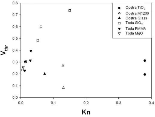
Concerning microgravity conditions, Toda, Ohi, Dobashi, and Hirano (1996), Toda, Ohnishi, Dobashi, and Hirano (1998) and Oostra (1998) per-formed experiments in the drop tower facilities of JAMIC (g0= 10−5g, t =

10 s) and Zarm, in Bremen and the results are shown in Fig. 2.2

Toda et al. (1996, 1998) carried out experiments in Knudsen number range of 0.008-0.15, using SiO2, MgO and PMMA particles in air at

atmo-spheric pressure.

Toda’s microgravity experiments gave values of Vthr as much as two or

three times higher than those predicted by Talbot’s equation, in experiments performed with SiO2, and about seven times higher with MgO (k = 1.4 and

42 W m−1_K−1_{, respectively).}

Oostra’s results obtained with TiO2 , M1200 (silica powder, Merk,

Ger-many) and glass (k=11.7, 1.01 and 0.93 W m−1_K−1_{, respectively) are lower}

than the values predicted by Talbot’s equation. These experimental results have a large uncertainty due to the fact that the aerosol used in the experi-ments has a broad particle size distribution.

Prodi et al. (2006) performed experiments in microgravity conditions so as to obtain measurements of thermophoretic velocities in the transition re-gion, using aerosol particles with different thermal conductivities (carnauba wax, paraffin and sodium chloride) and nitrogen as carrier gas. The aim was to evaluate the influence of the thermal conductivity of the particles in the thermophoresis.

The present work reports on the last test series of experiments (Octo-ber 2005) whose main goal was to obtain thermophoretic velocities in

(41)

mi-Figure 2.2: Reduced thermophoretic velocity as a function of the Knudsen number. Experimental data of Oostra (1998) and Toda et al. (1996, 1998) are reported.

(42)

crogravity conditions for gases with different thermal conductivities. Such experiments were never done before.

The data were compared with the theories of Talbot et al.(1980), Ya-mamoto and Ishihara (1988), and Beresnev and Chernyak (1995).

These theories, as shown above, have a different approach to the ther-mophoresis phenomenon.

2.3 Experimental set-up

As told in the introduction, in normal gravity it is not possible to study the phoretic effect alone, as particles move due to gravity and due to nat-ural convection resulting from temperature gradients established to study thermophoresis. So experiments were performed in microgravity conditions. The microgravity experiments were carried in the drop tower facility, which provides a weightlessness stage of about 4.7 s under free fall conditions with residual acceleration of about 10−6_g

0. The experimental apparatus is

housed in a special pressurized capsule (see Fig 2.3).

The electronic system of the Bremen drop tower comprises a ground station computer system, a telemetry remote control-transmission line, and a capsule computer system inside the capsule itself, allowing the control and automation of the experiment.

The cell used for the experiments consists of two plane plates (18.5 x 18.5 mm2_{), one at the top and one at the bottom of the square mono-block}

vessel of optically polished Pyrex. The distance between the plates was 7 mm (see Fig. 2.4)

The upper plate was heated by an electric heater, and the lower one was maintained at ambient temperature. The temperature of the bottom and top of the cell was measured and recorded 2 times per second with two thermocouples inserted in the plates as sensors.

The heating of the upper plate started 3 min before the beginning of the microgravity condition and switched off 5 s after the fall. As the time required to heat the upper plate is about 1 min, when the capsule begins to drop, the temperature of the plate is completely stabilized. The standard deviation of temperature measured during the falls is about 0.1 and 0◦_{C for}

the upper and bottom plate, respectively.

(43)

(44)

Figure 2.4: An example of cell used for experiments

bottom plate, which shut immediately after the introduction of the aerosol assuring a good seal. Using the electronic system of the drop tower, the aerosol was automatically injected into the cell about 15 s before the free fall (beginning of microgravity), and the flow was stopped about 2 s prior to the capsule drop.

The temperature and pressure inside the capsule were continuously mon-itored. N2, Ar, He and Xe were supplied during the runs with small

pres-surized bottle (1 or 10 l). The temperature gradient in the cell during the runs performed with N2 as carrier gas was in the range 4215-5730 K m−1 ,

with He in the range 1270-1900 K m−1_{, Ar in the range 4760-5060 K m}−1 _,

and Xe in the range 4790-5310 K m−1_.

The aerosol inside the cell was observed through the digital holographic velocimeter (Dubois, Joannes, & Legros, 1999), a device allowing the deter-mination of 3-D coordinates of particles (30 frames/s; space resolution of about 0.2 m) in the viewing volume of 0.5 x 0.5 x 0.5 mm3_{. Particle}

tra-jectories were reconstructed through the analysis of the sequence of particle positions, and a mean velocity for each particle was calculated by dividing

(45)

the length of the trajectory of each considered particle by the time employed. For each drop the number of frames recorded in microgravity conditions was about 130.

In order to calculate the velocity of each particle, the initial frame was considered to be that in which the gas motion was stopped and the movement of particles was vertical, i.e. in the direction of the thermal gradient.

The characteristic time of momentum transfer, i.e. the time necessary to allow the velocity of the gas inside the cell to be negligible when micro-gravity conditions are established, is theoretically related to δ2_{/ν(δ, distance}

between the plate; ν, kinematic viscosity), and should be theoretically about 1 s for Xe and lower for N2, He, and Ar (Dressler, 1981).

It is important to note that it was possible to check the actual relaxation time for momentum by observing the recorded images; from this inspection it turned out that the time was lower than 0.4 s for He, N2 and Ar, while it was about 2 s for Xe. Therefore, for Ar, He, N2, it was possible to measure

in each run the velocity of an individual particle for a maximum time of 4 s, and for Xe for about 2.5 s.

The relaxation time for aerosol particle was much lower than the mo-mentum relaxation time.

Tab. 3Values of physical parameters for Ar, Xe, He, N2

Gas λ, µm Tmean,K λ, µm kg, W m−1K−1 η,N s m−2 v,m2s−1

at T=293.15K at Tm atTmean atTmean (at Tmean)

Ar 0.069 315.79 0.07582 0.0185 2.388E-5 1.54E-5 Ar 0.069 315.25 0.07535 0.0185 2.377E-5 1.53E-5 Ar 0.069 316.6 0.07606 0.0185 2.394E-5 1.55E-5 Xe 0.0382 314.85 0.04182 0.058 2.432E-5 4.91E-5 Xe 0.0382 316.4 0.04208 0.058 2.444E-5 4.95E-5 Xe 0.0382 314.95 0.04183 0.058 2.433E-5 4.91E-5 Xe 0.0382 316.5 0.04209 0.058 2.444E-5 4.95E-5 He 0.189 302.6 0.19677 0.1558 2.006E-5 1.24E-5 He 0.189 304.6 0.19842 0.1558 2.015E-5 1.26E-5 N2 0.0676 314 0.07375 0.0207 1.86E-5 1.70E-5

(46)

Figure 2.5: Monodisperse aerosol generator (Mage)

aerosol generator (Minimage, see Figure 2.5), a modified version of MAGE (Prodi, 1972).

The measured value of thermal conductivity of paraffin turned out to be 0.42 W m−1_K−1_{. The thermal conductivity of carrier gases N}

2, Ar, Xe and

He was found to be 0.0195, 0.0178, 0.0054, 0.153 W m−1 _K −1 _{at T =293}

K, respectively.

In order to calculate the thermophoretic force and compare the exper-imental results with the current theories on thermophoresis (Beresnev & Chernyak, 1995; Talbot et al., 1980; Yamamoto & Ishihara, 1988) and simi-lar terrestrial experiments (Jacobsen & Brock, 1965; Schmitt, 1959), it was necessary to consider some physical parameters, which are reported in Table 3. The mean free path was calculated from (Chen & Xu, 2002; Kennard, 1938; Saxton & Ranz,1952)

(47)

where m is the mass of a gas molecule; n the molecular number density; p the gas pressure; v the average thermal speed given by

v = [8kBT /(πm)]0.5, (2.6)

where η is the gas viscosity; kB the Boltzmann’s constant; T the gas

tem-perature; and ρ the gas density.

The values used for the viscosities of the gases are from Gray (1972). The translational thermal conductivity was calculated from

kg = (

15

4 )Rη/M = ( 15

4 )ηkB/m, (2.7)

where M is the gas molecular weight (g mol−1_{); and R, the universal gas}

constant.

The thermophoretic force, which is equal to drag force in steady state, was calculated from

Fth= 6πηrVth/S, (2.8)

where Vth is the experimental thermophoretic velocity, S is the slip

correc-tion;

S = 1 + Kn[A1+ A2exp(−A3/Kn)]. (2.9)

Experiments on different gases (Ar, N2, CO2, H2) and substances (paraffin,

silicon oil) show that A1, A2 and A3 values can be considered independent

of gases (Schmitt, 1959).

In order to calculate the experimental reduced thermophoretic force Fth/(r2dT /dy), we assumed A1 = 1.155; A2 = 0.471; A3 = 0.596 for all

the gases (Allen & Raabe, 1982).

2.4 Results

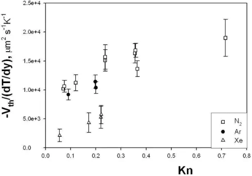
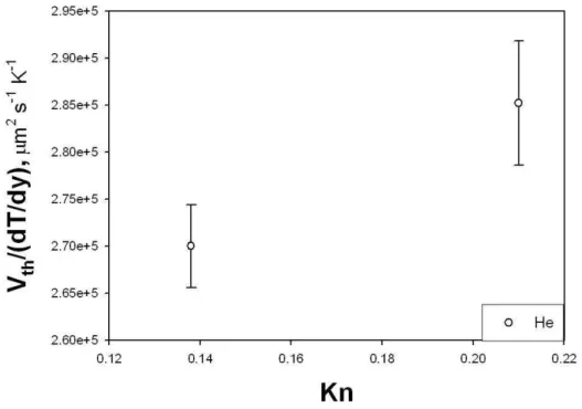
Figs. 2.6 and 2.7 and report the thermophoretic velocity (Eq.), normal-ized to 315 K, vs. Knudsen number, obtained from microgravity experiments

(48)

Figure 2.6: Experimental data for the normalized thermophoretic velocity vs. Knudsen number (Ar, Xe, and N2 as carrier gas).

performed on different gases. It can be observed that the thermophoretic velocity decreases from He, N2, Ar, Xe.

In order to explain this trend, it must be borne in mind that one of the factors determining the movement of an aerosol particle in the presence of a thermal gradient is thermal creep. Utilizing gas kinetic theory, Maxwell (1879) predicted that the tangential temperature gradient ∇T at a gas-solid surface would cause a thin layer of gas adjacent to the surface to move with

u = cs∇T/T, (2.10)

where ν is the kinematic viscosity of the gas, and cs is the thermal slip

coefficient.

The thermal creep turns out to be proportional to the kinematic viscosity of the gas. The present experimental data show that the thermophoretic velocity has the same trend as ν, i.e. the highest value is for He with the highest kinematic viscosity, and the lowest for Xe, which has the lowest ν.

(49)

(50)

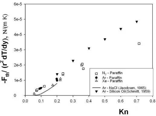
Figure 2.8: Experimental data and Waldmann’s solution for the normalized thermophoretic force.

Fig.2.8 shows the experimental reduced thermophoretic force Fth/(r2dT /dy)

vs. Knudsen number, and the theoretical equation of Waldmann for N2 in

the free-molecule regime (8.8 x 10−5_{N m}−1_K−1 _{at T = 293 K).}

In the Waldmann region (Kn ≫ 1), where drag force is proportional to velocity and the square of the particle radius, and the thermophoretic force is proportional to the square of the radius, the thermophoretic velocity is independent of Kn and of the thermal conductivity of the particles.

Experimental data show that the reduced thermophoretic force (F_th−r) can be considered a unique function of the Kn number (range 0.05-0.8) for

N2, Ar and Xe.

This can be explained if it is considered that, by equating Fth and drag

force, it turns out that