Università degli Studi di Salerno
CELPE
Centro di Economia del Lavoro e di Politica Economica
Carmen AINA*, Fernanda MAZZOTTA**, Lavinia PARISI**
**Dipartimento di Economia (DiSEI) - Università del Piemonte Orientale
**Università degli Studi di Salerno - CELPE
Bargaining or efficiency within the household?
The case of Italy
Corresponding author
Scientific Commitee
Adalgiso AMENDOLA, Floro Ernesto CAROLEO, CESARE IMBRIANI, Marcello D’AMATO, Pasquale PERSICO C.E.L.P.E.
Centro di Ricerca Interdipartimentale di Economia del Lavoro e di Politica Economica Università degli Studi di Salerno
Via Giovanni Paolo ii, 132 - 84084 Fisciano, I- Italy
http://www.celpe.unisa.it
Index
Abstract ... 5
Introduction ... 7
1. Data and definition of dependent variables ... 8
1.1 Descriptive statistics ... 9
2. Method ... 11
3. Estimates ... 12
4. Conclusion ... 14
Bargaining or efficiency within the household? The case of Italy
Carmen AINA*, Fernanda MAZZOTTA**, Lavinia PARISI**
**Dipartimento di Economia (DiSEI) - Università del Piemonte Orientale
**Università degli Studi di Salerno - CELPE
Abstract
Two aspects play a role in the household decision-making, the efficiency and the bargaining power’s argument. The crucial difference between the two approaches is the expected influence of personal and partners’ wage. To investigate which of the two models hold, in the Italian context, we estimate an ordered probit model for five aspects of household decision-making. We use the Italian questionnaire of Statistics on Income and Living Conditions (It-Silc) 2010 as it provides a module on intra-household sharing of resources. Results show that in strategic control decisions, where the power argument should dominate the efficiency approach (i.e. decisions on durable goods, savings and other important decisions) the spouse/partner with higher wage is the household decision maker. For decision regarding executive management (i.e. decision on everyday shopping), the efficiency argument holds.
Keywords Financial management, Intra-household bargaining, Household production, Gender differences; Intra-household decision power; Family economics
Introduction
This paper aims at providing evidence on the determinants of intra-household decision-making power with respect to several outcomes, namely everyday shopping, purchase of durable goods, savings and taking relevant decisions. Exploring the process through which spouses/partners take a decision is important for better targeting any household policy interventions. In addition, from the economic viewpoint, it is important to analyse the degree of involvement of family members in economic decisions to state the consumer behaviour.
In fact, the recent growing interest in understanding the household decision-making is driven by the effects that power’s distribution amongst components exerts on key economic outcomes, such as female labour force participation, how resources are distributed within the family, how household decisions are made in a variety of economic and non-economic contexts. A better knowledge of the determinants of power between partners can also provide significant information on gender inequality in household decision-making as well as its evolution over time. Unfortunately, the empirical evidence on this topic is lacking of well-established results, mainly because the evaluation of the spouse/partner’s power within the family is difficult to source because of the lack of detailed and useful data, which are based, once available, on self-reported measures. For instance, questions about who makes some decisions suffers from some important limitations as their interpretation can vary according to different individuals. Overall, several empirical studies consider that the comparative resources like income, education, health conditions, family size, age gap, and occupational status of spouses/partners play a significant role in the balance of power (see for instance Bertocchi et al., 2012). Further measures of bargaining power explored in the literature refer to the socio-economic environment, since social norms, cultural beliefs, and economic conditions are estimated to be relevant distribution factor in the household decision-making framework. A well-documented result is that economic variables, especially measured in terms of differences in the level of income and occupational status, are key factors in determining the most powerful partner. Gender differences emerge once the spouse/partner who takes the decision within the family is analysed. In particular, women are generally more risk averse, so once they are the decision maker in the household they tend to make less risky investments (see, Sundén and Surette, 1998; Jianakoplos and Barnasek, 1998; Barber and Odean, 2001; Guiso and Jappelli, 2002; Croson and Gneezy, 2009). It has also been found that income given to women is more likely to be used for investments in education, children’s nutrition and housing (Thomas, 1990; Duflo, 2003). Other studies underline that for women the degree of power in managing household’s decisions is positively correlated with their level of education and their status in the labour market (Lührmann and Maurer, 2007; Elder and Rudolph, 2003).Woolley (2003) finds that the spouse/partner with the higher income is the one taking decisions in the household. Additional contributions provide evidence that who controls the income in the family - male or female - directly affects decisions and outcomes within the household, for instance in terms of child health and education, and expenditures for different goods and services (see Lundberg et al. 1997; Phipps and Burton, 1998; Duflo, 2003).
In the economic literature, it is crucial to define, for a better interpretation of the distribution of power in the households, the theoretical framework in which family makes decisions, since household outcomes result from decisions made by spouses/partners. Consequently, the particular conditions under which a decision is made in the family matters. Chiefly, two theoretical models can be considered to deepen the household decision-making processes: the unitary and the bargaining model. The former approach underlines the hypothesis that households behave as a single decision unit where both spouses/partners have the same preferences or one of them takes all the decisions to somehow maximizes the welfare of its members, under the hypothesis of income pooling (Becker, 1991; Dobbelsteen and Kooreman, 1997), ignoring intra-household decisions completely. This model refers to a household production approach, where both spouses/partners allocate efficiently their time in all the family activities. Basically, it is assumed that partners freely decide how to allocate time to income work activities, to home production activities (i.e. the outcomes selected in our investigation: as everyday shopping, etc.), and to leisure, which are all exogenously determined. As a result, optimal decision-making entails that the spouse/partner with the lower
opportunity costs - measured in terms of income foregone - should devote more time to family production activities. It is clear that the partner in question is the one who is either not working or with the lower wage. The bargaining model, instead, assumes that each individual in the family has distinct preferences towards spending available household income, hence the final decision is the product of negotiation amongst partners rather than a choice driven by a single agent (Nash, 1950; Rubenstein, 1982). The optimal allocation of time results from the household maximizing its utility subjects to certain time, budget constraints and home production function, weighted by his/her power. Thence, in case of egoistic agents, each spouse/partner will maximize only his or her utility function, yielding a situation where the couple manages separately their resources and consumption. While, in case of cooperative behaviour between partners, the individual with higher wage rate has a greater bargaining power, hence he/she will raise his/her share in household financial management.
Accordingly, in our empirical exercise for each outcome we test the prevailing model analysing the different effect plays by income. In the unitary model, the household decision maker is the spouse/partner with the lower opportunity cost, hence the one with the lowest wage. Consequently, a negative effect of income on each decision outcome entails that both partners’ time inputs into household management result from an efficient distribution of labour within the couple. While, the bargaining framework suggests that the spouse/partner who earns more, namely who has his/her wage positively correlated with the outcome, is the final decision maker. Accordingly, we may expect that the household production model may hold for routinely, less time-consuming and less important decisions. By contrast, the bargaining argument should be predominant for important and infrequent decisions.
Following the theoretical frameworks described, we provide evidence of which model holds for each outcome in the Italian context. Using data drawn from the Italian questionnaire of Statistics on Income and Living Conditions (It-Silc), we estimate the role of spouse/partner’s characteristics in different decisions, ranked according to their degree of relevance. Results show that in strategic control decisions, where the power argument should dominate the efficiency approach (such as decisions on durable goods, savings and important decisions) a positive correlation between wages and degree of power played by the spouse/partner is found. By contrast, about decision related to executive management (for example decision on everyday shopping), in which the household production approach should dominate, the bargaining power argument holds.
The paper is organized as follows. The next section offers a description of the data. Section 3 discusses the empirical strategy. Section 4 provides the corresponding results. Finally, conclusions are reported in section 5.
1.
Data and definition of dependent variables
We make use of the 2010 Italian questionnaire of Statistics on Income and Living Conditions (It-Silc) as it provides a module on the list of target secondary variables relating to intra-household sharing of resources. The data are based on a standardized questionnaire filled by individuals and households in several European countries and on several issues. The Italian component (It-Silc) contains information on demographic characteristics, personal income, housing conditions, employment and so on at household and individual‘s level. Any component of the family, aged 16 and over, is eligible to answer the questionnaire. Chiefly, we focus on five variables related to five different aspects of decision making within the family. We define those variables as follows and we report the corresponding questions: the first concerns EverydayShopping, the question is: “Thinking of you and your spouse or partner, who is more likely to take decisions on everyday shopping?” All expenses on everyday shopping are to be covered, including expenses made by the respondent for himself or herself.
The second variable is named Durable as it concerns decision on durable goods, the associated question is the following: “Thinking of you and your spouse or partner, who is more likely to take decisions on expensive purchases of consumer durables and furniture?”. Durable consumption includes one-off purchases of items such as white goods (fridges,
washing-machines), larger pieces of furniture, electrical appliances, and so on, acquired by households for final consumption (i.e. those that are not used by households as stores of value or by unincorporated enterprises owned by households for purposes of production). These items may be used for purposes of consumption repeatedly or continuously over a period of a year or more (source OECD).
The third variable is about Borrowing money; partners are asked to answer the following question: “Thinking of you and your spouse or partner, who is more likely to take decisions on borrowing money?”.The respondent has to include the decisions on mortgages and loans, too. The fourth variable is about Savings, and couples are asked to answer the following questions: “Thinking of you and your spouse or partner, who is more likely to take decisions on the use of savings?”.
The final variable is related to ImportantDecision. The associated question is the following: “Thinking of you and your spouse or partner who is, on the whole, more likely to have the last word when taking important decisions?”
The aforementioned questions are addressed to the same target population i.e. persons aged 16 and over living in a household with at least a partner living in the household. They reflect different aspect of decision making grades from the less important (first variable) to the most important (fifth variable).
Moreover, the different questions reveal different types of decision making authority, in particular, according to Vogler and Pahl (1994), it is plausible to distinguish between strategic control (i.e. important and infrequent decision such as decisions on durable goods, borrowing money and savings) and executive management (i.e. decision that are time consuming such as everyday shopping) decisions.
The individual level is vital for this question as it asks for a subjective perception of decision making in the household. Consequently, we look at personal level answer even though there is inconsistency in the responses. Inconsistency emerges when the partners in the couple provide different answers to the same question; if, for example, both persons in the household answer that they are more likely to take decisions on a specific subject.
The variable are coded as follows: (i) 1 More me (i.e. I decide), (ii) 2 Balanced (i.e. we both decide), (iii) 3 More my partner (i.e. my partner decides). The variables 2 and 3 have additional values in the responses, first there is an additional code defined as the decision has never arisen, and for the variable 3 an additional one defined as we do not have common savings. However, those values are filled by a small number of individuals, less than 1% that’s why we include them in the missing category.
Finally, we recode the dependent variable in order to be interpreted always as women power (i.e. the higher the code to more likely the wife to decide) in both men and women estimates.
1.1 Descriptive statistics
Table 1 reports descriptive statistics of our dependent variables. For each question the answers of each respondent within the couple has been shown. Individuals can answer to each question in three different ways: I decide, we both decide, my partner decides. We cross the answers of males and females and in the table the rows report the percentages of males answering on the specific item, while the columns underline the corresponding figure for women.
Table 1 shows that roughly, the 88% of the cases1 agree about who decides on daily shopping, and more than half of respondents report to take decision on everyday shopping jointly. Everyday shopping can be seen as a time-consuming activity and a routine-like decision, hence the efficiency argument is probably more persuasive and the household production approach may hold (Dobbelsteen and Kooreman 1997). The role of the women in this context is well established, in fact 33.3% of men report that their spouse/partner completely decide about everyday shopping while only the 5.8% state that they decide by themselves. Overall 48.9% of the family decide together on everyday shopping. The
percentage of men and women answering that they are the only responsible for the everyday shopping is higher than the percentage stated by their spouses/partners: for instance 38.8% of females declare that they decide on this item, while 37.2% of males answer that their partners decide on it (the corresponding figure is 8.1% and 7.6% for males).
Woman's answer
EverydayShopping Durable goods
MAN BOTH WOMAN Total MAN BOTH WOMAN Total
Ma n 's am sw er MAN 5.8% 1.5% 0.8% 8.1% 8.8% 2.1% 0.3% 11.3% BOTH 1.0% 48.9% 4.7% 54.7% 1.6% 78.7% 1.2% 81.5% WOMAN 0.7% 3.2% 33.3% 37.2% 0.3% 1.8% 5.1% 7.3% Total 7.6% 53.6% 38.8% 100.0% 10.8% 82.6% 6.6% 100.0% Borrowing Saving MAN 9.9% 2.1% 0.3% 12.3% 7.0% 1.9% 0.2% 9.1% BOTH 1.8% 80.9% 0.9% 83.6% 2.4% 81.2% 1.2% 84.9% WOMAN 0.2% 1.0% 2.9% 4.1% 0.4% 1.7% 3.9% 6.0% Total 11.9% 84.1% 4.0% 100.0% 9.8% 84.8% 5.3% 100.0% Important decision MAN 10.9% 2.6% 0.7% 14.3% BOTH 1.8% 71.7% 2.1% 75.6% WOMAN 0.5% 2.0% 7.6% 10.2% Total 13.3% 76.3% 10.4% 100.0%
Table 1 (cell percentages)
The question is “Thinking of you and your spouse or partner, who is more likely to take decisions on…?”
About decisions regarding strategic control, i.e. important and infrequent decision (see for instance Vogler and Pahl 1994) such as purchasing durable goods as well as decision on savings, we notice that the common practice is to decide all together. About 80% of couples decide together on durable goods (78.8%), borrowing money (80.9%), and savings decisions (81.2%). In contrast with executive management, in the choices where the power aspect may dominate the efficiency argument, only few women decide on their own (5.1% for durable goods, 2.9% for borrowing money and 3.9 % on savings)2. Another important difference observed in Table 1 is on the discrepancy in the answers. Partners sometimes disagree, as we do find discrepancy in the answers, i.e. partners do not answer in the same way to the question. The highest relative percentage of disagreement corresponds to the figure on everyday shopping. There are several explanations for the discrepancies in the answers provided and the most convincing one, in our opinion, is that respondents are not aware of their authority within the family. Of course it could be also that men and women perceive the world differently and\or they do not want to admit any authority of their partners. Sometimes partners overestimate their power, in particular, in our sample, for daily decisions, sometimes partners underestimate their decision’s power within the family, for instance, in our sample, for important and infrequent decisions. In fact, females underestimate their power within the family with regards of durable goods and savings, in fact only 5.3% (6.6% for durable goods) of them think they can decide on their own, while 6.0% (7.3% for durable goods) of males
2
answer that their partners decide. By contrast, male tend to over-estimate their power in all the decisions, but savings.
About the distribution of answers for the Important Decision, in other words, who take the final decision on the purchase of important items; males prefer to have the last word, as 10.9% of them think they can decide on their own. Only 7.6 % of women has such power.
Finally, among strategic control decisions we can distinguishes between infrequent decisions such as purchasing durable goods where the cooperation (partners answering ‘we both take this decision’) between partners is high and important decisions such as who has the final word where the cooperation is low. What emerges is a sort of specialization within the couple: women in the daily expensive and men in important decisions (i.e. ‘who has the right of the last word’). This could be not intuitive given that we should expect that financial decisions would have been those showing a higher level of specialization but they are usually taken together.
2.
Method
As we have already described, two aspects (i.e. household production model and bargaining model) play a role in the household decision making (see Dobbelsteen and Kooreman, 1997) and the crucial difference between the two is the expected influence of partners’ wage. To investigate which of the two model hold, in the Italian context, we estimate an ordered probit model for each of the five aspect of household decision making. We use observations for both spouses/partners and we discuss only estimates on the sample restricted to couples for which both spouses/partners have chosen the same answer categories. However, we test our
assumptions also for all the sample including the observations for which there is no agreement amongst the partners and the results are still in line with the restricted sample.
The relevant variable to check, whether the prediction of the model holds, is the wage rate of the partners. We believe that potential wage is most important in explaining the two approaches than actual wage. This is because the actual wage can be determined both from a personal decision on whether accepting or not a job along with the degree of difficulties to find a job in the labour market. Moreover, it can be determined by partner’s wage. A woman with a positive value on income means that she has a paid job and this may provide bargaining power in another form: woman who works outside their home may learn social and other skills needed to navigate the work environment and this may translate back into increased bargaining power within the house (Doss, 2012). To disentangle the effect of potential wage on decision making, we use four approaches: first we include in the estimation the education of both partners as a proxy of potential wage, second we include also a dummy indicating whether the wage of the partner is higher than the one of the respondent. Third, we use the predicted wages imputed to the all sample and estimated by a wage equation that uses only individual that do have wages. Finally, we use the actual wage imputing the predicted only to individuals that have no wages3.
We also define the categories to ease interpretation in the bargaining framework: the power of women is Dijw*k and it increases with higher value of the codes in the answer: Di0wk is the
probability that the man takes the decision, Di1wk is the probability that both partners take the
decision and Di2wk is the probability that woman decides. We take into consideration five types
of decisions identified by k. Then, we estimate separately for men and women the following ordered probit:
Dijw*k = β1yim + β2yiw + α’X + ui (1) With k=1,…, 5 and i=1,…, N Where yim and yiw are the variables of interest such as wages (as defined above) and Xis a set
of control variables (such as age, age difference, health, whether cohabiting, and so on). We test whether β1 and β2, are greater or not than zero. Considering Di0wk if β1≤0 and β2≥0
household production model holds, otherwise power argument may be used to interpret
3
Results on wage equation are not reported for the sake of brevity but are available upon request. Moreover for the specification with the potential income we calculate the boostrap standard errors.
results. Considering Di2wk if β1≥0 and β2≤0 household production model holds, otherwise power
argument may be used to interpret results. We expect that the income of women have less effect on the decision of men given women are usually secondary earner in family, then β2
should be less significant.
We consider also the potential income estimating separately for individual younger than 65 (i.e. we estimate for them labour income) and individual older than 64 (i.e. we estimate for them pension income). 4The estimated income take into consideration the opportunity cost of reduce or give away a work and this is more important for women that are the ones with a lot of zero for income variable. Moreover, we expected that women engaged in time consuming decisions (such as daily shopping) are also those that have greater difference between potential and effective income, for this reason when considering Di0wk , β2≤0 for potential
income and β2≥0 for actual income, while when considering Di2wk the opposite is true.
3.
Estimates
As stated, the dependent variables considered have three different values going from 1 to 3 suggesting that at the higher value is associated a greater female’s power. Consequently, the dependent variable, for both men and women, has to be interpreted as a measure of women’s power in taking decisions. The interpretation of a negative (positive) coefficient on a particular covariates means that the wife is less (more) likely to decide. Tables 2a and 2b show estimates for the sample of couples for which partners have agreed with the answers. To ease the interpretation of results we also provide marginal effects for all the outcomes (see Tables 3a-7b). We remind to the reader that the coding of the answer is the following: 1 if man takes the decision, 2 if both spouses/partners take the decision and 3 if female decides. We are aware that our final sample (Tab.2a and 2b) could be a selected one given that partners agreed on answer, but results are still robust and do not change when also not homogeneous answers are included. 5
In each estimate, we include four different specifications, which are reported in separate columns, namely (i) wage proxied by the level of education of both partners, (ii) dummy on whether the partner’s wage is higher than the respondent’s wage, (iii) the potential wage imputed for all sample as described above (iv) the actual wage for the entire sample. The potential wage is predicted for each individual in the sample according to the estimation of a wage equation using the Heckman approach (estimates of Heckman probit are not reported here but are available upon request). The wage equation is calculated on those individuals who report a positive wage separated for men and women and we distinguish between income from labour and income from pension. For labour income, regressors in the wage equation are age, education and geographical area, while the restriction variable is number of components less than 16 years old. For income composed by pension, the explanatory variables in the income equation are education, if a person has ever worked and his/her health’s conditions while the restriction variable is age.
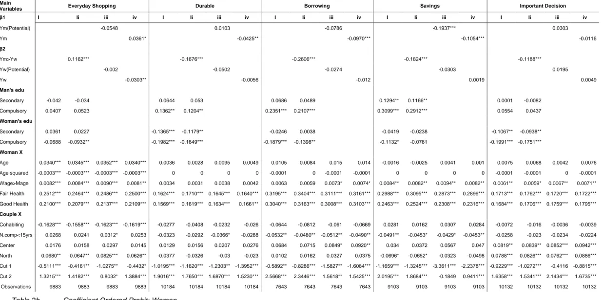
Table 2a and 2b reports estimates for men and women, respectively. Focusing on the main variables (i.e. income) we find that, β1 is positive and/or β2 is negative for executive
management decision (i.e. decision on everyday shopping), thus for such item the assumption of household production model holds. However, for strategic control decisions (i.e. decisions on durable goods, borrowing, savings and important decisions) the power argument dominates the efficiency approach given that β1 is negative and/or β2 is positive. Overall, every
time women have a higher level of education, they are more likely to decide, and this result still holds when we include a dummy controlling for the situation where the partner has a greater income than respondent has. The effect is stronger for men about decisions on durable goods and important decision. Regarding the bargaining power model, we do find that
4
We estimate four wage equations as described in the next section.(two for labour income and to for pension income and for males and females).
5
for decision about important and infrequent items if the man has higher income than woman,, he is more likely to decide.
Furthermore, when we include potential and actual wage, we do find the same predictions: for everyday shopping decisions, the higher the actual wage of the individual the less likely is the probability that he/she decides. The opposite is true for decisions on durable goods, on savings and important decisions. Thus, the power argument holds. This result may entail that the breadwinner within the family plays a central role when the amount to be spent is important, while he/she empowers the partner for less costly expenditures.
Looking at the marginal effects (Tables 3a-7b) we can analyse the effect of the aforementioned variables on the probability that the man is the decision making, the probability that both partners take the decision and the probability that woman decides. In particular we find that if the man is the breadwinner in the household the power of the wife increases on everyday shopping decisions (about of 4.4 percentage points - pp). This result suggests an efficiency way of assigning tasks and responsibility within the family. Moreover, we do find that it is much important in explaining the decision power within the family the difference in wages than the level of them. In fact, the dummy variable regarding whether the partner has an income higher than the respondent is always significant and, for everyday shopping decisions, it increases the probability that the woman decides of about 4.4 (pp). This is the highest effect of this variable given that for strategic control decision (purchase of durable goods, borrowing, savings and important decisions) if man (woman) has higher income than his (her) partner, the probability that woman decides decreases (increases) of about 2 pp. In these last decisions in fact, the power arguments holds given that individuals with higher income are the ones who decide regardless the gender (the corresponding figure for men is about 2.6 pp for durable goods, 4.3 pp for borrowing and 2.4 pp for saving and important decisions). Thus, the estimates underline that the person who takes decisions is the individual that earns more in the family. The log of potential income is not significantly different from zero in almost all equations. For important decisions we do find that it increases the probability that a woman decides of about 1 pp (men’s equation) and for savings we find that the log of men potential income increases the probability that he decides of about 2 pp (men’s estimates) and 3 pp (women’s estimates). With regard to the actual income, it decreases the probability that a partner takes decision on everyday shopping of about 0.5 pp for men and 1.2 pp for women (Table 3a and 3b). Moreover for decisions on durable goods purchase, borrowing money and savings only males’ income is significantly difference from zero and it reduces the probability that a woman decides of about, 0.5 pp, 0.7 pp and 0.9 pp, respectively (Tab. 4b, 5b and 6b). This is true also when we look at man estimates (Tab. 4a, 5a and 6a) but the effect is slightly higher. Concerning the everyday shopping decisions, once we control for females’ potential income in the males’ equation, the greater probability of being a decision maker for females (about 2.5 pp) reveals that there is a positive difference between the potential income and actual income for women more devoted to daily time-consuming activities instead of being at work.
With reference to the other control variables, it seems that female’s power increases as age elapsed by, reaching the maximum at age 50 once we consider the outcome about everyday shopping decision. Up to 50 years old, the higher the age the less likely is male to decide according to his spouse/partner, after 50 years old this relationship is at the opposite. Table 2b reports estimates for men and results do not underline any differences between men and women on age, expect for the turning point that for men is around 53 years of age. However, when we take into consideration the differences in age of the spouses/partners, we notice that the spouse/partner that he/she is older than the other one is the one who is more likely to take decision. Especially, with regard to everyday shopping, the probability of being the one who decide is larger for men than for women, when men are older than their spouses/partners. Moreover, we do find differences in age among decisions. In particular, for everyday shopping and saving decisions the probability that men decide increases by 0.03 and 0.05 pp for any additional year of age, however it decreases by 0.05 pp on durable goods decisions and it is not significant in other strategic control decisions. Not surprisingly, health is strongly correlated with everyday decisions: individuals with bad health are more likely to let their partner deciding for each decision considered, and this is true regardless the respondent and the specifications considered. We also find that cohabiting people instead of married couple are more likely to
take decisions on everyday shopping jointly, suggesting a more collaborative behaviour in couple not legally related. In case of non-cooperation in everyday shopping is the man who is in charge of taking the decision. Particularly, men who cohabit declare that are more likely to decide on their own (about 2 pp) or with their partner (about 4 pp) than those who are married. When the male is the one who earns more in the household, the women is more likely to take everyday shopping decisions, but if we include in the specification the women’s potential income, we find that females are more likely either to take joint decisions or to leave the responsibility to her spouse/partner. Education plays a role only in strategic control decisions where the more educated partner is the one who decides. Not surprisingly, we do not find differences in all the decisions regarding to health: unhealthy individuals leave their partners to decide more frequently. Moreover, only for important or on everyday shopping decisions, we find significant geographical differences, namely in the North women have more power than in the South given that their partners leave them to decide more often with regard the aforementioned questions (1.3pp and 3pp, respectively).
Finally, looking at the observed and predicted probabilities, we can see that for strategic control decisions, couples are more likely to decide all together (around 80%), while for executive management decision only 50% of couple declare that they both decide. In fact, for the last category (i.e. everyday shopping) it is more likely that wives decide..
4.
Conclusion
This paper aimed at investigating the determinants of intra-household decision-making power with respect to several outcomes, namely everyday shopping, purchase of durable goods, savings and taking relevant decisions. In particular, our goal has been to test two potential models: the first related to a household production (efficiency) approach, where both spouses/partners allocate efficiently their time in all the family activities. The optimal allocation of time results from the household maximizing its utility subject to certain time and budget constraints and the home production function. Alternatively, in the second model, financial management is a reflection of bargaining power. Thus in this framework both partners have diverse utility functions, so their preferences may differ.
What emerges is that the household production model shows a negative correlation between a partner’s wage rate and his/her participation in financial management while the second model predicts a positive correlation between a partner’s wage rate and with whom he/she is the decision making.
Using data drawn from the It-Silc 2010, we estimated the role of spouse/partner’s characteristics in several decisions, ranking the answers provided according to the degree of power given to women. Results show that in strategic control decisions, where the power argument should dominate the efficiency approach (such as decisions on durable goods, savings and important decisions) a positive correlation between wages and the degree of powerful played by the spouse/partner is found. We estimate that the presence of a higher income of one partner decreases the decision’s probability of the other. By contrast, with regard to decisions related to executive management (for example decisions on everyday shopping), in which the household production approach should dominate, the opposite is true. Overall, what emerges is that there is a specialization within the family on time-consuming activities, with females more devoted to daily decisions (i.e. everyday shopping decisions), but the breadwinner in the family is the one who is more active in taking more costly decisions, such as purchase of durable goods and borrowing decisions.
References
Barber, B.M., Odean, T., 2001. Boys will be boys: Gender, overconfidence and common stock investments. Quarterly Journal of Economics, 116, 261-289.
Becker, G., 1991. A Treatise on the Family, Enlarged Edition, Cambridge, Massachussetts: Harvard University Press.
Bertocchi, G. Brunetti M. and Torricelli C. 2012. Is it money or brains? The determinants of intra-family decision power. ChilD n. 2/2012.
Croson, R., Gneezy, U., 2009. Gender differences in preferences. Journal of Economic Literature, 47, 448-474.
Dobbelsteen, S., Kooreman, P., 1997. Financial management, bargaining and efficiency within the household: An empirical analysis. De Economist, 145, 345-366.
Doss, C., 2012. Intrahaousehold bargaining and resource allocation in developing countries. World Development Report.
Duflo, E., 2003. Grandmothers and granddaugthers: old age pension and intra-household allocation in South Africa. World Bank Review, 17, 1-25.
Elder, H.W., Rudolph, P.M., 2003. Who makes the financial decisions in the households of older Americans? Financial Services Review, 12, 293-308.
Guiso, L., Jappelli, T., 2002. Household portfolios in Italy. In Guiso, L., Haliassos, M., Jappelli, T. (Eds.), Household Portfolios. MIT Press: Cambridge.
Jianakoplos, N.A., Bernasek A., 1998. Are women more risk averse? Economic Inquiry, 36, 620-630.
Lührmann, M., Maurer, J., 2007. Who wears the trousers? A semiparametric analysis of decision power in couples. CeMMAP Working Paper CWP25/07.
Lundberg, S., Pollak, R.A., Wales, T.J., 1997. Do husband and wives pool their resources? Evidence from the UK child benefit. Journal of Human Resources, 22, 463-480.
Nash, J., 1950. The Bargaining Problem. Econometrica, 181, 155-162.
Phipps, S., Burton, P., 1998. What’s mine is yours? The influence of male and female income on pattern of household expenditure. Economica, 65, 599-613.
Rubenstein, A., 1982. Perfect Equilibrium in a bargaining model. Econometrica, 50, 97-109.
Sundén, A.E., Surette, B.J., 1998. Gender differences in the allocation of assets in retirement savings plans. American Economic Review, 88, 207-211.
Thomas, D., 1990. Intra-household resource allocation: an inferential approach. Journal of Human Resources, 25(4), 635-64.
Vogler, C., Pahl, J. 1994. Money, power and inequality within marriage. The Sociological Review, 42(2), 263-288.
Woolley, F., 2003. Control over money in marriage. In Grossbard-Shechtman, S.A. (Ed.), Marriage and the economy: Theory and evidence from advanced industrial societies. Cambridge University Press: New York.
Everyday Shopping Durable Borrowing Savings Important Decision
I Ii iii iv i ii iii iv i ii iii iv i ii iii iv i ii iii iv
Main Variables β1 Ym(Potential) -0.0317 0.0597 -0.0117 -0.1360** 0.0592 Ym 0.0455*** -0.0286 -0.0802*** -0.0871*** -0.0026 β2 Yw>Ym -0.1146*** 0.1650*** 0.2655*** 0.1769*** 0.1301*** Yw(Potential) 0.0657** 0.0139 0.0656 0.0466 0.0655 Yw -0.0233 0.00 0.002 0.0115 0.0097 Man's edu Secondary -0.0391 -0.0317 0.0628 0.0523 0.0616 0.0431 0.1244** 0.1126** 0.0005 -0.008 Compulsory 0.0307 0.041 0.1183** 0.1042* 0.2040*** 0.1819*** 0.2805*** 0.2640*** 0.0436 0.0321 Woman's edu Secondary 0.0292 0.0155 -0.1411*** -0.1224** -0.0287 0.001 -0.0457 -0.0275 -0.1113** -0.0968** Compulsory -0.0821* -0.1075** -0.2117*** -0.1776*** -0.2018*** -0.1504** -0.1245** -0.0873 -0.2103*** -0.1831*** Man X Age 0.0270*** 0.0271*** 0.0188*** 0.0260*** -0.0056 -0.0059 -0.0105 -0.0054 -0.0029 -0.0037 -0.0119 0.0001 -0.0151* -0.0155* -0.0195* -0.0132 0.0031 0.0027 -0.0083 0.0022 Age squared -0.0003*** -0.0003*** -0.0002*** -0.0003*** 0.0001 0.0001 0.0001 0.0001 0.00 0.00 0.0001 0.00 0.0001 0.0001 0.0001 0.0001 0.00 0.00 0.0001 0.00 Mage>Wage -0.0059** -0.0061** -0.0064** -0.0053 -0.0074** -0.0070** -0.0073* -0.0075* -0.0084** -0.0078* -0.0086** -0.0086* -0.0061 -0.0058 -0.0066 -0.0061 -0.0048 -0.0045 -0.0052 -0.0047 Fair Health -0.1363*** -0.1380*** -0.1394*** -0.1390*** -0.2743*** -0.2737*** -0.2716*** -0.2719*** -0.2636*** -0.2650*** -0.2721*** -0.2683*** -0.3455*** -0.3451*** -0.3508*** -0.3475*** -0.1985*** -0.1978*** -0.1979*** -0.1971*** Good Health -0.1451*** -0.1495*** -0.1433*** -0.1520*** -0.3124*** -0.3084*** -0.3131*** -0.3023*** -0.3008*** -0.2954*** -0.3083*** -0.2903*** -0.4079*** -0.4037*** -0.4196*** -0.4134*** -0.2091*** -0.2055*** -0.2049*** -0.1987*** Couple X Cohabiting -0.1748*** -0.1686*** -0.1742*** -0.1730*** -0.0394 -0.0515 -0.0362 -0.0373 -0.0835 -0.0994 -0.0799 -0.0832 0.0144 0.0039 0.0188 0.0165 -0.0156 -0.0247 -0.0133 -0.0122 N.comp<15yr s 0.0194 0.0169 0.0296 0.0176 -0.0352* -0.0323 -0.0361* -0.0323* -0.0557** -0.0507** -0.0484** -0.0515** -0.0550** -0.0516** -0.0440* -0.0518** -0.029 -0.0264 -0.0232 -0.026 Center 0.0215 0.0203 0.026 0.0187 0.0159 0.018 0.0127 0.0302 0.0705 0.0723 0.0708* 0.0933** 0.0361 0.0381 0.0458 0.0481 0.0855** 0.0868** 0.0819** 0.0975*** North 0.0766*** 0.0743*** 0.0774*** 0.0705** -0.0277 -0.0238 -0.0382 -0.0149 0.0182 0.0223 0.013 0.0427 -0.0592 -0.0566 -0.0438 -0.0426 0.0879*** 0.0907*** 0.0735** 0.0963*** Cut 1 -0.8713*** -0.8918*** -0.8306* -0.7704*** -1.7647*** -1.7301*** -1.3602*** -1.9975*** -1.5153*** -1.4708*** -1.8201*** -2.3554*** -1.7749*** -1.7342*** -2.7614*** -2.4374*** -1.3028*** -1.2685*** -0.1495 -1.2862*** Cut 2 0.8597*** 0.8400*** 0.8993** 0.9598*** 0.9204*** 0.9584*** 1.3223*** 0.6858** 1.3948*** 1.4519*** 1.0801* 0.5494* 1.1196*** 1.1656*** 0.1255 0.4524 1.0496*** 1.0867*** 2.2001*** 1.0627*** Observations 9883 9883 9883 9883 10184 10184 10184 10184 7643 7643 7643 7643 9103 9103 9103 9103 10132 10132 10132 10132 Table 2a Coefficient Ordered Probit: Men
Main
Variables Everyday Shopping Durable Borrowing Savings Important Decision
β1 I Ii iii iv I Ii iii iv I Ii iii iv I Ii iii iv I Ii iii iv
Ym(Potential) -0.0548 0.0103 -0.0786 -0.1937*** 0.0303 Ym 0.0361* -0.0425** -0.0970*** -0.1054*** -0.0116 β2 Ym>Yw 0.1162*** -0.1676*** -0.2606*** -0.1824*** -0.1188*** Yw(Potential) -0.002 -0.0502 -0.0274 -0.0303 0.0195 Yw -0.0303** -0.0056 -0.012 0.0019 0.0049 Man's edu Secondary -0.042 -0.034 0.0644 0.053 0.0686 0.0489 0.1294** 0.1166** 0.0001 -0.0082 Compulsory 0.0407 0.0523 0.1362** 0.1204** 0.2351*** 0.2107*** 0.3099*** 0.2912*** 0.0554 0.0437 Woman's edu Secondary 0.0361 0.0227 -0.1365*** -0.1179** -0.0246 0.0038 -0.0419 -0.0238 -0.1067** -0.0938** Compulsory -0.0688 -0.0932** -0.1982*** -0.1649*** -0.1879*** -0.1398** -0.1132* -0.0761 -0.1991*** -0.1751*** Woman X Age 0.0340*** 0.0345*** 0.0352*** 0.0340*** 0.0036 0.0028 0.0095 0.0049 0.0105 0.0084 0.015 0.014 -0.0016 -0.0025 0.0041 0.001 0.0075 0.0068 0.0042 0.0076 Age squared -0.0003*** -0.0003*** -0.0003*** -0.0003*** 0 0 0 0 -0.0001 0 -0.0001 -0.0001 0 0 0 0 -0.0001 -0.0001 0 -0.0001 Wage>Mage 0.0082*** 0.0084*** 0.0090*** 0.0081** 0.0034 0.0031 0.0038 0.0042 0.0063 0.0059 0.0073* 0.0074* 0.0084** 0.0082** 0.0094** 0.0082** 0.0061** 0.0059* 0.0067** 0.0071** Fair Health 0.2512*** 0.2464*** 0.2486*** 0.2500*** 0.1624*** 0.1710*** 0.1645*** 0.1640*** 0.3195*** 0.3404*** 0.3111*** 0.3161*** 0.2988*** 0.3095*** 0.2873*** 0.2896*** 0.1713*** 0.1762*** 0.1720*** 0.1722*** Good Health 0.2100*** 0.2079*** 0.2137*** 0.2109*** 0.1569*** 0.1619*** 0.1634*** 0.1661** 0.3040*** 0.3163*** 0.3008*** 0.3103*** 0.2463*** 0.2524*** 0.2308*** 0.2316*** 0.1684*** 0.1706*** 0.1759*** 0.1795*** Couple X Cohabiting -0.1628*** -0.1558*** -0.1623*** -0.1619*** -0.0277 -0.0408 -0.0232 -0.026 -0.0644 -0.0812 -0.061 -0.0669 0.0281 0.0162 0.0307 0.0284 -0.0072 -0.016 -0.0036 -0.0039 N.comp<15yrs 0.0268 0.0241 0.0312* 0.0253 -0.0323 -0.0292 -0.0366* -0.0288 -0.0532** -0.0480** -0.0512** -0.0490** -0.0491** -0.0453* -0.0429* -0.0453** -0.0258 -0.023 -0.0234 -0.0224 Center 0.0176 0.0158 0.0297 0.0145 0.0129 0.0156 0.0207 0.0276 0.0684 0.0715 0.0849* 0.0920** 0.034 0.0372 0.0567 0.047 0.0819** 0.0839** 0.0852*** 0.0942*** North 0.0680** 0.0647** 0.0825*** 0.0626** -0.0377 -0.0326 -0.03 -0.023 0.0102 0.0162 0.0327 0.0375 -0.0696* -0.0652* -0.0323 -0.0498 0.0788*** 0.0826*** 0.0762*** 0.0886*** Cut 1 -0.5111*** -0.4161** -1.0275** -0.4432* -1.0195*** -1.1620*** -1.2303** -1.3952*** -0.5892** -0.8286*** -1.5827** -1.6084*** -1.1659*** -1.3245*** -3.3611*** -2.2378*** -0.9229*** -1.0272*** -0.4116 -0.8815*** Cut 2 1.3215*** 1.4182*** 0.8032* 1.3884*** 1.9016*** 1.7650*** 1.6870*** 1.5230*** 2.5668*** 2.3446*** 1.5618** 1.5425*** 2.0195*** 1.8684*** -0.1849 0.9411*** 1.6358*** 1.5341*** 2.1434*** 1.6735*** Observations 9883 9883 9883 9883 10184 10184 10184 10184 7643 7643 7643 7643 9103 9103 9103 9103 10132 10132 10132 10132
VARIABLES Man takes decision Both take decision Woman takes decision Man takes decision Both take decision Woman takes decision Man takes decision Both take decision Woman takes decision Man takes decision Both take decision Woman takes decision Main Variables β1 Ym(Potential) 0.0038 0.00838 -0.0122 Ym -0.00534*** -0.0122** 0.0176** β2 Yw>Ym 0.0142*** 0.0295*** -0.0437*** Yw(Potential) -0.00789** -0.0174** 0.0253**
Yw 2.73E-03 6.25E-03 -8.99E-03
Man's edu Secondary 0.00473 0.0103 -0.015 0.00386 0.0083 -0.0122 Compulsory -0.00352 -0.00837 0.0119 -0.00471 -0.0112 0.0159 Woman's edu Secondary -0.00317 -0.00821 0.0114 -0.00164 -0.0044 0.00604 Compulsory 0.00974* 0.0219* -0.0316* 0.0126** 0.0288** -0.0414** Man X Age 0.000290** 0.000667** -0.000957** 0.000283** 0.000653** -0.000936** 0.000306** 0.000675** -0.000981** 0.000366*** 0.000839** -0.00121*** Mage>Wage 0.000685** 0.00157** -0.00226** 0.000712** 0.00164** -0.00235** 0.000766** 0.00169** -0.00245** 0.00062 0.00142* -0.00204* Fair Health 0.0145*** 0.0388*** -0.0533*** 0.0146*** 0.0394*** -0.0540*** 0.0152*** 0.0391*** -0.0543*** 0.0147*** 0.0397*** -0.0544*** Good Health 0.0155*** 0.0412*** -0.0567*** 0.0159*** 0.0425*** -0.0584*** 0.0157*** 0.0401*** -0.0558*** 0.0163*** 0.0431*** -0.0594*** Couple X Cohabiting 0.0230*** 0.0429*** -0.0659*** 0.0220*** 0.0416*** -0.0636*** 0.0234*** 0.0419*** -0.0653*** 0.0228*** 0.0424*** -0.0652*** N.comp<15yrs -0.00226 -0.0052 0.00747 -0.00197 -0.00455 0.00652 -0.00356 -0.00783* 0.0114 -0.00206 -0.00473 0.00679 Center -0.00263 -0.00559 0.00822 -0.00248 -0.0053 0.00779 -0.00326 -0.00665 0.00991 -0.00229 -0.00486 0.00715 North -0.00900*** -0.0205*** 0.0295*** -0.00870*** -0.0199*** 0.0286*** -0.00934** -0.0204*** 0.0297*** -0.00830** -0.0189** 0.0272*** N.Obs. 9,883 9,883 9,883 9,883 9,883 9,883 9,883 9,883 9,883 9,883 9,883 9,883 Obs. Prob. 6.64% 55.58% 37.78% 6.64% 55.58% 37.78% 6.64% 55.58% 37.78% 6.64% 55.58% 37.78% Pred.Prob. 5.86% 54.36% 39.77% 5.85% 54.39% 39.77% 6.05% 54.73% 39.21% 5.88% 54.36% 39.76% Table 3a Marginal Effect at Mean - Everyday Shopping Men
VARIABLES Man takes decision Both take decision Woman takes decision Man takes decision Both take decision Woman takes decision Man takes decision Both take decision Woman takes decision Man takes decision Both take decision Woman takes decision Main Variables β2 Yw(Potential) 0.000231 0.000559 -0.000791 Yw 0.00344** 0.00828* -0.0117* β1 Ym>Yw -0.0140*** -0.0305*** 0.0445*** Ym(Potential) 0.00621 0.015 -0.0212 Ym -0.00410** -0.00986** 0.0140* Woman's edu Secondary -0.00384 -0.0102 0.0141 -0.00236 -0.00651 0.00887 Compulsory 0.00796 0.0186 -0.0265 0.0107** 0.0253* -0.0360** Men's edu Secondary 0.00498 0.0111 -0.0161 0.00405 0.009 -0.013 Compulsory -0.00452 -0.0113 0.0158 -0.00583 -0.0145 0.0203 Woman X Age 0.0000411 0.0000987 -0.00014 0.0000324 0.0000783 -0.000111 0.000139 0.000337 -0.000476 0.000083 0.000199 -0.000282 Wage>Mage -0.000934*** -0.00224*** 0.00318*** -0.000950*** -0.00229*** 0.00324*** -0.00101*** -0.00245*** 0.00347*** -0.000923*** -0.00222*** 0.00314** * Fair Health -0.0322*** -0.0627*** 0.0949*** -0.0315*** -0.0616*** 0.0931*** -0.0319*** -0.0620*** 0.0939*** -0.0321*** -0.0623*** 0.0944*** Good Health -0.0278*** -0.0511*** 0.0788*** -0.0273*** -0.0508*** 0.0781*** -0.0281*** -0.0522*** 0.0803*** -0.0279*** -0.0513*** 0.0792*** Couple X Cohabiting 0.0207*** 0.0410*** -0.0617*** 0.0196*** 0.0395*** -0.0591*** 0.0205*** 0.0411*** -0.0616*** 0.0205*** 0.0408*** -0.0614*** N.comp<15yrs -0.00305 -0.00733 0.0104 -0.00273 -0.0066 0.00934 -0.00354* -0.00856* 0.0121* -0.00287 -0.0069 0.00977 Center -0.00209 -0.00467 0.00676 -0.00187 -0.00422 0.00608 -0.00353 -0.00788 0.0114 -0.00171 -0.00385 0.00556 North -0.00775** -0.0185** 0.0263** -0.00735** -0.0177** 0.0250** -0.00941*** -0.0225** 0.0319*** -0.00713** -0.0171** 0.0242* N.Obs. 9,883 9,883 9,883 9,883 9,883 9,883 9,883 9,883 9,883 9,883 9,883 9,883 Obs. Prob. 6.64% 55.58% 37.78% 6.64% 55.58% 37.78% 6.64% 55.58% 37.78% 6.64% 55.58% 37.78% Pred.Prob. 5.65% 54.14% 40.20% 5.63% 54.15% 40.22% 5.63% 54.00% 40.37% 5.65% 54.11% 40.24% Table 3b Marginal Effect at Mean - Everyday Shopping Women
VARIABLES Man takes decision Both take decision Woman takes decision Man takes decision Both take decision Woman takes decision Man takes decision Both take decision Woman takes decision Man takes decision Both take decision Woman takes decision Main Variables β1 Ym(Potential) -0.0103 0.00407 0.00627 Ym 0.00488 -0.00184 -0.00305 β2 Yw>Ym -0.0262*** 0.00712*** 0.0191*** Yw(Potential) -0.00242 0.000953 0.00146
Yw 2.24E-06 -8.43E-07 -1.40E-06
Man's edu Secondary -0.0115 0.0054 0.00609 -0.00948 0.00438 0.0051 Compulsory -0.0209** 0.00889* 0.0120** -0.0183* 0.00767 0.0106** Woman's edu Secondary 0.0214*** -0.00406*** -0.0173*** 0.0189*** -0.00429*** -0.0146** Compulsory 0.0337*** -0.00906*** -0.0246*** 0.0284*** -0.00816*** -0.0203*** Man X Age -0.000537** 0.000204** 0.000333** -0.000522** 0.000199** 0.000323** -0.000513** 0.000202* 0.000311* -0.000404* 0.000152* 0.000252 Mage>Wage 0.00127** -0.000482** -0.000788** 0.00120** -0.000456** -0.000739** 0.00126** -0.000498* -0.000766** 0.00129* -0.000485** -0.000804** Fair Health 0.0389*** -0.00272 -0.0362*** 0.0389*** -0.00305 -0.0358*** 0.0391*** -0.00346 -0.0356*** 0.0389*** -0.00316 -0.0358*** Good Health 0.0456*** -0.00547* -0.0402*** 0.0450*** -0.00556* -0.0394*** 0.0464*** -0.00659* -0.0398*** 0.0443*** -0.00534* -0.0389*** Couple X Cohabiting 0.00689 -0.00282 -0.00407 0.00905 -0.0038 -0.00524 0.0064 -0.0027 -0.00371 0.00651 -0.00264 -0.00388 N.of comp<15y rs 0.00602* -0.00229* -0.00373* 0.0055 -0.0021 -0.0034 0.00626* -0.00247** -0.00379** 0.00552* -0.00208* -0.00344* Center -0.00267 0.000927 0.00174 -0.003 0.00106 0.00195 -0.00214 0.00076 0.00138 -0.00507 0.00176 0.00331 North 0.00476 -0.00185 -0.00291 0.00409 -0.0016 -0.0025 0.00665 -0.00267 -0.00398 0.00258 -0.00101 -0.00158 Observations 10,184 10,184 10,184 10,184 10,184 10,184 10,184 10,184 10,184 10,184 10,184 10,184 Observed Probability 9.54% 84.91% 5.55% 9.54% 84.91% 5.55% 9.54% 84.91% 5.55% 9.54% 84.91% 5.55% Predicted Probability 9.65% 85.17% 5.18% 9.62% 85.24% 5.14% 9.83% 85.05% 5.11% 9.66% 85.12% 5.22% Table 4a Marginal Effect at Mean - Durable- Men
VARIABLES Man takes decision Both take decision Woman takes decision Man takes decision Both take decision Woman takes decision Man takes decision Both take decision Woman takes decision Man takes
decision Both take decision
Woman takes decision Main Variables β2 Yw(Potential) 0.00836 -0.00274 -0.00562 Yw 0.000942 -0.000327 -0.000616 β1 Ym>Yw 0.0263*** -0.00646*** -0.0198*** Ym(Potential) -0.00172 0.000565 0.00116 Ym 0.00715* -0.00248* -0.00467** Woman's edu Secondary 0.0206*** -0.00354** -0.0170** 0.0181** -0.00383** -0.0143** Compulsory 0.0312*** -0.00758*** -0.0236*** 0.0262*** -0.00690*** -0.0193*** Men's edu Secondary -0.0118 0.00544 0.00634 -0.00961 0.00437 0.00524 Compulsory -0.0238** 0.00958** 0.0142*** -0.0209** 0.00832* 0.0126** Woman X Age -0.00101*** 0.000356*** 0.000650*** -0.000986*** 0.000353*** 0.000634*** -0.000848*** 0.000278*** 0.000570*** -0.000910*** 0.000315*** 0.000594*** Wage>Mage -0.000573 0.000203 0.000371 -0.00052 0.000186 0.000334 -0.000625 0.000205 0.00042 -0.000709 0.000246 0.000463 Fair Health -0.0298*** 0.0138** 0.0160*** -0.0313*** 0.0146** 0.0167*** -0.0299** 0.0134* 0.0165*** -0.0302** 0.0140** 0.0161*** Good Health -0.0289*** 0.0135** 0.0154*** -0.0298*** 0.0142** 0.0157*** -0.0297** 0.0133* 0.0164*** -0.0305*** 0.0142** 0.0164*** Couple X -0.00574 Cohabiting 0.00475 -0.00179 -0.00297 0.00703 -0.00274 -0.00429 0.00392 -0.00136 -0.00256 0.00445 -0.00163 -0.00317 N.of comp<15 yrs 0.00546 -0.00193 -0.00353 0.00493 -0.00176 -0.00317 0.00608* -0.00200* -0.00409* 0.00485* -0.00168 0.00312 Center -0.00212 0.000662 0.00146 -0.00256 0.000819 0.00174 -0.00335 0.000968 0.00239 -0.00453 0.00141 -0.00251 North 0.00641 -0.00232 -0.00409 0.00554 -0.00203 -0.00351 0.00502 -0.00170 -0.00332 0.00392 -0.00141 0.000594*** N. Obs. 10,184 10,184 10,184 10,184 10,184 10,184 10,184 10,184 10,184 10,184 10,184 10,184 Obs. Prob. 9.54% 84.91% 5.55% 9.54% 84.91% 5.55% 9.54% 84.91% 5.55% 9.54% 84.91% 5.55% Pred. Prob. 9.49% 85.14% 5.37% 9.47% 85.21% 5.32% 9.30% 85.16% 5.54% 9.45% 85.12% 5.43% Table 4b Marginal Effect at Mean - Durable- Women
VARIABLES Man takes decision Both take decision Woman takes decision Man takes decision Both take decision Woman takes decision Man takes decision Both take decision Woman takes decision Man takes decision Both take decision Woman takes decision Main Variables β1 Ym(Potential) 0.00218 -0.00144 -0.000747 Ym 0.0145*** -0.00921*** -0.00532*** β2 Yw>Ym -0.0431*** 0.0231*** 0.0200*** Yw(Potential) -0.0122 0.00805 0.00419
Yw -3.61E-04 2.29E-04 1.32E-04
Man's edu Secondary -0.0126 0.00932 0.00331 -0.00869 0.00639 0.0023 Compulsory -0.0385*** 0.0258*** 0.0127*** -0.0338*** 0.0226** 0.0112*** Woman's edu Secondary 0.0046 -0.00236 -0.00224 -0.000172 0.0000955 0.0000769 Compulsory 0.0363*** -0.0228*** -0.0135*** 0.0273** -0.0177*** -0.00958** Man X Age -0.000235 0.000151 0.0000837 -0.000202 0.000131 0.0000707 -0.000137 0.0000901 0.0000469 -0.0000497 0.0000315 0.0000182 Mage>Wage 0.00153** -0.000987** -0.000547** 0.00141* -0.000913* -0.000492* 0.00161** -0.00106** -0.000552** 0.00156* -0.000987** -0.000570* Fair Health 0.0403*** -0.0182*** -0.0221*** 0.0405*** -0.0189*** -0.0216*** 0.0425*** -0.0199*** -0.0226*** 0.0412*** -0.0186*** -0.0226*** Good Health 0.0472*** -0.0228*** -0.0245*** 0.0461*** -0.0226*** -0.0235*** 0.0494*** -0.0246*** -0.0248*** 0.0453*** -0.0213*** -0.0240*** Couple X Cohabiting 0.0159 -0.0108 -0.00507 0.019 -0.0132 -0.00582* 0.0155 -0.0108 -0.00478 0.0158 -0.0106 -0.00516 N. comp<15 rs 0.0101** -0.00653** -0.00362** 0.00919** -0.00597** -0.00322** 0.00903* -0.00594* -0.00309* 0.00933** -0.00592** -0.00342** Center -0.0127 0.00802 0.00468 -0.013 0.00828 0.00467 -0.0130* 0.00837 0.00464 -0.0168** 0.0105** 0.00626* North -0.00338 0.00223 0.00115 -0.00413 0.00275 0.00137 -0.00247 0.00167 0.000804 -0.00793 0.0052 0.00273 N. Obs. 7,643 7,643 7,643 7,643 7,643 7,643 7,643 7,643 7,643 7,643 7,643 7,643 Obs. rob. 10.61% 86.34% 3.05% 10.61% 86.34% 3.05% 10.61% 86.34% 3.05% 10.61% 86.34% 3.05% Pred.Prob. 10.54% 86.62% 2.84% 10.46% 86.78% 2.76% 10.89% 86.33% 2.78% 10.45% 86.63% 2.91% Table 5a Marginal Effect at Mean - Borrowing Men
VARIABLES Man takes decision Both take decision Woman takes decision Man takes decision Both take decision Woman takes decision Man takes decision Both take decision Woman takes decision Man takes decision Both take decision Woman takes decision Main Variables β2 Yw(Potential) 0.00484 -0.00292 -0.00191 Yw 0.00212 -0.00129 -0.000829 β1 Ym>Yw 0.0415*** -0.0214*** -0.0201*** Ym(Potential) 0.0139 -0.00839 -0.00549 Ym 0.0171*** -0.0104*** -0.00668*** Woman's edu Secondary 0.00387 -0.00191 -0.00196 -0.000614 0.000329 0.000285 Compulsory 0.0330*** -0.0200*** -0.0130*** 0.0248** -0.0156** -0.00918** Men's edu Secondary -0.014 0.0103 0.00372 -0.00983 0.0072 0.00263 Compulsory -0.0434*** 0.0283*** 0.0151*** -0.0384*** 0.0251*** 0.0133*** Woman X Age -0.000883*** 0.000548*** 0.000335*** -0.000839*** 0.000528*** 0.000311*** -0.000646* 0.000391** 0.000256** -0.000736*** 0.000449** 0.000288** Wage>Mage -0.00112 0.000698 0.000427 -0.00104 0.000655 0.000386 -0.00129* 0.000778* 0.000509* -0.00130* 0.000794 0.000509* Fair Health -0.0660*** 0.0489*** 0.0172*** -0.0704*** 0.0527*** 0.0177*** -0.0638*** 0.0465*** 0.0173*** -0.0653*** 0.0481*** 0.0172*** Good Health -0.0634*** 0.0473*** 0.0161*** -0.0663*** 0.0503*** 0.0160*** -0.0621*** 0.0455*** 0.0166*** -0.0643*** 0.0475*** 0.0168*** Couple X Cohabiting 0.0119 -0.00773 -0.00413 0.015 -0.0101 -0.005 0.0111 -0.00706 -0.00405 0.0122 -0.00787 -0.00437 N.comp<15rs 0.00947** -0.00587** -0.00359** 0.00852** -0.00536** -0.00316** 0.00904** -0.00546** -0.00357** 0.00864* -0.00527** -0.00338** Center -0.012 0.00723 0.00474 -0.0125 0.00769 0.0048 -0.0148* 0.00883* 0.00602* -0.0161* 0.00965* 0.00644** North -0.00184 0.00118 0.00067 -0.00294 0.00190 0.00103 -0.00590 0.00370 0.00220 -0.00678 0.00429 0.00249 N. Obs. 7,643 7,643 7,643 7,643 7,643 7,643 7,643 7,643 7,643 7,643 7,643 7,643 Obs. rob. 10.61% 86.34% 3.05% 10.61% 86.34% 3.05% 10.61% 86.34% 3.05% 10.61% 86.34% 3.05% Pred.Prob. 10.18% 86.84% 2.97% 10.14% 86.99% 2.87% 10.07% 86.83% 3.09% 10.08% 86.87% 3.05% Table 5b Marginal Effect at Mean - Borrowing - Women
VARIABLES Man takes decision Both take decision Woman takes decision Man takes decision Both take decision Woman takes decision Man takes decision Both take decision Woman takes decision Man takes decision Both take decision Woman takes decision Main Variables β1 Ym(Potential) 0.0200** -0.00883** -0.0112** Ym 0.0126*** -0.00530*** -0.00730*** β2 Yw>Ym -0.0235*** 0.00728*** 0.0162*** Yw(Potential) -0.00686 0.00303 0.00384
Yw -1.66E-03 6.98E-04 9.61E-04
Man's edu Secondary -0.0215** 0.0134* 0.00812** -0.0192* 0.0119* 0.00739** Compulsory -0.0439*** 0.0226*** 0.0213*** -0.0409*** 0.0208*** 0.0201*** Woman's edu Secondary 0.00609 -0.00189 -0.00419 0.00374 -0.00131 -0.00243 Compulsory 0.0176** -0.00690** -0.0107* 0.0124 -0.00507 -0.00733 Man X Age 0.000446* -0.000191* -0.000255** 0.000459** -0.000198* -0.000261** 0.000488** -0.000215** -0.000273** 0.000452** -0.000190* -0.000262** Mage>Wage 0.000887 -0.00038 -0.000507 0.000835 -0.00036 -0.000475 0.000965 -0.000425 -0.000539 0.000879 -0.00037 -0.000509 Fair Health 0.0382*** 0.00101 -0.0392*** 0.0382*** 0.000582 -0.0388*** 0.0391*** 0.000922 -0.0400*** 0.0382*** 0.00191 -0.0401*** Good Health 0.0475*** -0.00331 -0.0442*** 0.0469*** -0.00349 -0.0434*** 0.0495*** -0.00403 -0.0455*** 0.0480*** -0.00257 -0.0454*** Couple X Cohabiting -0.00206 0.000861 0.0012 -0.000561 0.00024 0.000321 -0.00273 0.00117 0.00157 -0.00237 0.000963 0.0014 N. comp<15yrs 0.00797** -0.00342** -0.00455** 0.00746** -0.00321** -0.00425** 0.00648** -0.00286** -0.00362* 0.00749** -0.00315** -0.00434** Center -0.00496 0.00176 0.0032 -0.00521 0.00187 0.00334 -0.00643 0.00243 0.00399 -0.00663 0.00236 0.00427 North 0.00871 -0.00389 -0.00482 0.0083 -0.00373 -0.00457 0.00655 -0.00302 -0.00353 0.00627 -0.00277 -0.00349 N. Obs. 9,103 9,103 9,103 9,103 9,103 9,103 9,103 9,103 9,103 9,103 9,103 9,103 Obs. rob. 7.65% 88.14% 4.22% 7.65% 88.14% 4.22% 7.65% 88.14% 4.22% 7.65% 88.14% 4.22% Pred.Prob. 7.74% 88.45% 3.81% 7.70% 88.52% 3.77% 7.90% 88.32% 3.78% 7.72% 88.42% 3.87% Table 6a Marginal Effect at Mean - Saving - Men
VARIABLES Man takes decision Both take decision Woman takes decision Man takes decision Both take decision Woman takes decision Man takes decision Both take decision Woman takes decision Man takes decision Both take decision Woman takes decision Main Variables β2 Yw(Potential) 0.00424 -0.00153 -0.00272 Yw -0.000265 0.0001 0.000165 β1 Ym>Yw 0.0237*** -0.00626*** -0.0174*** Ym(Potential) 0.0271*** -0.00974*** -0.0173*** Ym 0.0149*** -0.00561*** -0.00928*** Woman's edu Secondary 0.00549 -0.00151 -0.00398 0.00319 -0.00102 -0.00218 Compulsory 0.0157* -0.00552** -0.0101* 0.0106 -0.00395 -0.00666 Men's edu Secondary -0.0224** 0.0137** 0.00864** -0.0199* 0.0121* 0.00781** Compulsory -0.0476*** 0.0230*** 0.0246*** -0.0443*** 0.0212*** 0.0231*** Woman X Age -0.0000953 0.000037 0.0000583 -0.0000752 0.0000295 0.0000457 0.0000911 -0.0000328 -0.0000584 -0.000113 0.0000424 0.0000701 Wage>Mage -0.00119** 0.000461** 0.000727** -0.00116** 0.000455** 0.000703** -0.00131** 0.000471** 0.000838*** -0.00116* 0.000435** 0.000720** Fair Health -0.0481*** 0.0258*** 0.0223*** -0.0498*** 0.0270*** 0.0228*** -0.0452*** 0.0228** 0.0224*** -0.0460*** 0.0238*** 0.0222*** Good Health -0.0410*** 0.0235*** 0.0175*** -0.0421*** 0.0246*** 0.0176*** -0.0377*** 0.0206** 0.0171*** -0.0382*** 0.0214*** 0.0168*** Couple X Cohabiting -0.00392 0.00142 0.00249 -0.00227 0.000861 0.00141 -0.00422 0.0014 0.00282 -0.00394 0.00139 0.00255 N.of comp<15yrs 0.00695** -0.00270* -0.00426** 0.00641* -0.00252* -0.00389* 0.00600** -0.00216* -0.00384** 0.00640** -0.00241** -0.00399** Center -0.00453 0.00136 0.00317 -0.00495 0.00152 0.00343 -0.00758 0.00223 0.00535 -0.00631 0.0019 0.00441 North 0.0100* -0.00406* -0.00594* 0.00936* -0.00386* -0.00551* 0 0 0 0.00716 0 0 N. Obs. 9,103 9,103 9,103 9,103 9,103 9,103 9,103 9,103 9,103 9,103 9,103 9,103 Obs. rob. 7.65% 88.14% 4.22% 7.65% 88.14% 4.22% 7.65% 88.14% 4.22% 7.65% 88.14% 4.22% Pred.Prob. 7.51% 88.45% 4.03% 7.49% 88.53% 3.98% 7.38% 88.42% 4.20% 7.48% 88.41% 4.11% Table 6b Marginal Effect at Mean - Saving - Women
VARIABLES Man takes decision Both take decision Woman takes decision Man takes decision Both take decision Woman takes decision Man takes decision Both take decision Woman takes decision Man takes decision Both take decision Woman takes decision Main Variables β1 Ym(Potential) -0.012 0.00311 0.00892 Ym 0.000513 -0.000112 -0.000402 β2 Yw>Ym -0.0244*** 0.00312*** 0.0213*** Yw(Potential) -0.0133 0.00345 0.00987*
Yw -1.92E-03 4.18E-04 1.50E-03
Man's edu Secondary -0.000106 0.0000278 0.0000781 0.00161 -0.000412 -0.0012 Compulsory -0.00864 0.00191 0.00673 -0.00634 0.00137 0.00497 Woman's edu Secondary 0.0196** -0.0000882 -0.0195** 0.0173** -0.000632 -0.0167** Compulsory 0.0395*** -0.00484** -0.0346*** 0.0346*** -0.00474*** -0.0298*** Man X Age 0.000369 -0.0000806 -0.000289 0.000381 -0.0000837 -0.000297 0.00036 -0.0000931 -0.000267 0.000580** -0.000126** -0.000453** Mage>Wage 0.000948 -0.000207 -0.000741 0.000888 -0.000195 -0.000693 0.00105 -0.000272 -0.000779* 0.00094 -0.000205 -0.000735 Fair Health 0.0353*** -0.000683 -0.0346*** 0.0352*** -0.000916 -0.0343*** 0.0363*** -0.00277 -0.0335*** 0.0354*** -0.00123 -0.0342*** Good Health 0.0374*** -0.00122 -0.0362*** 0.0368*** -0.00131 -0.0355*** 0.0378*** -0.00319 -0.0346*** 0.0357*** -0.00132 -0.0344*** Couple X Cohabiting 0.00312 -0.000723 -0.0024 0.00496 -0.00119 -0.00376 0.00273 -0.000735 -0.00199 0.00243 -0.000554 -0.00187 N. comp<15yrrs 0.00575 -0.00126 -0.00449 0.00521 -0.00114 -0.00407 0.00471 -0.00122 -0.00349 0.00516 -0.00112 -0.00403 Center -0.0173** 0.00436** 0.0129** -0.0175** 0.00448** 0.0131** -0.0169** 0.00474** 0.0121*** -0.0198*** 0.00500*** 0.0148*** North -0.0177*** 0.00444** 0.0133*** -0.0183*** 0.00460** 0.0137*** -0.0152** 0.00439** 0.0108** -0.0195*** 0.00497*** 0.0146*** N. Obs. 10,132 10,132 10,132 10,132 10,132 10,132 Obs. rob. 12.12% 79.48% 8.40% 12.12% 79.48% 8.40% 12.12% 79.48% 8.40% 12.12% 79.48% 8.40% Pred.Prob. 11.83% 79.73% 8.44% 11.81% 79.78% 8.41% 12.28% 79.57% 8.15% 11.87% 79.66% 8.47% Table 7a Marginal Effect at Mean - Important Decision - Men