Smartphone: An alternative to ground control points for orienting virtual outcrop models and assessing their quality

ABSTRACT

The application of structure from motion–multiview stereo (SfM-MVS) photogrammetry to map metric- to hectometric-scale exposures facilitates the production of three-dimensional (3-D) surface reconstructions with centimeter resolution and range error. In order to be useful for geospatial data interroga-tion, models must be correctly located, scaled, and oriented, which typically requires the geolocation of manually positioned ground control points with survey-grade accuracy. The cost and operational complexity of portable tools capable of achieving such positional accuracy and precision is a major obsta-cle in the routine deployment of SfM-MVS photogrammetry in many fields, including geological fieldwork. Here, we propose a procedure to overcome this limitation and to produce satisfactorily oriented models, which involves the use of photo orientation information recorded by smartphones. Photos captured with smartphones are used to: (1) build test models for evaluating the accuracy of the method, and (2) build smartphone-derived models of outcrops, used to reference higher-resolution models reconstructed from image data collected using digital single-lens reflex (DSLR) and mirrorless cameras. Our results are encouraging and indicate that the proposed workflow can produce registra-tions with high relative accuracies using consumer-grade smartphones. We also find that comparison between measured and estimated photo orientation can be successfully used to detect errors and distortions within the 3-D models.

INTRODUCTION

The application of structure from motion–multiview stereo (SfM-MVS) pho-togrammetry for generating three-dimensional (3-D) surface reconstructions of rock outcrops (virtual outcrop models, VOMs) has enjoyed rapid proliferation over the past decade (e.g., Sturzenegger and Stead, 2009; Favalli et al., 2012; Bemis et al., 2014; Bistacchi et al., 2015; Bisdom et al., 2016; Seers and Hodgetts, 2016; Tavani et al., 2016; Fleming and Pavlis, 2018; Hansman and Ring, 2019).

GEOSPHERE

GEOSPHERE; v. 15, no. 6 https://doi.org/10.1130/GES02167.1 5 figures; 1 table; 1 set of supplemental files CORRESPONDENCE: stefano.tavani@unina.it CITATION: Tavani, S., Corradetti, A., Granado, P., Snidero, M., Seers, T.D., and Mazzoli, S., 2019, Smartphone: An alternative to ground control points for orienting virtual outcrop models and assessing their quality: Geosphere, v. 15, no. 6, p. 2043–2052, https://doi.org /10.1130 /GES02167.1.

Science Editor: Andrea Hampel Associate Editor: Jose M. Hurtado Received 12 June 2019 Revision received 28 August 2019 Accepted 11 October 2019 Published online 8 November 2019

OPEN ACCESS GOLD

This paper is published under the terms of the CC‑BY‑NC license.

Smartphone: An alternative to ground control points for orienting

virtual outcrop models and assessing their quality

Stefano Tavani

1

_{, Amerigo Corradetti}

2

_{, Pablo Granado}

3

_{, Marco Snidero}

1,3

_{, Thomas D. Seers}

2

_{, and Stefano Mazzoli}

1,

_*

1_{Dipartimento di Scienze della Terra, dell’Ambiente e delle Risorse (DISTAR), Università degli Studi di Napoli Federico II, Napoli 80126, Italy}

2_{Department of Petroleum Engineering, Texas A&M University at Qatar, Doha, Qatar}

3_{Institut de Recerca Geomodels, Departament de Dinàmica de la Terra i de l’Oceà, Universitat de Barcelona, Barcelona 08028, Spain}

*Present address: School of Science and Technology, Geology Division, University of Camerino, Via Gentile III da Varano, 62032 Camerino, (MC), Italy

The fidelity of VOMs built using SfM-MVS photogrammetry now compares fa-vorably with that of models generated by terrestrial laser scanning (also known as terrestrial lidar) (Harwin and Lucieer, 2012; Nocerino et al., 2014), with rel-atively low cost and highly portable digital single-lens reflex (DSLR) or mir-rorless cameras enabling the construction of models with resolutions down to a few tens of microns (Corradetti et al., 2017). However, two major limita-tions of SfM-MVS photogrammetry still prevent its routine use in field geology. The first one is the common requirement for model registration during post- processing. The spatial registration of metric- to hectometric-scale outcrops, done within either a local or a global coordinate frame, typically requires the placement of ground control points (e.g., Javernick et al., 2014; James et al., 2017; Martínez-Carricondo et al., 2018) with centimeter to sub-centimeter (i.e., survey-grade) accuracy. Such levels of accuracy and precision can be achieved with a total station or using real-time kinematic differential global navigational satellite system (RTK-DGNSS) receivers (Carrivick et al., 2016). Such tools, how-ever, do not form part of the standard equipment of the field geologist, and are impractical to deploy, as they are expensive, cumbersome, and require special-ist operation. The second limitation of SfM-MVS models in virtual outcrop ge-ology is the occurrence of errors emanating from scene reconstruction (James and Robson, 2014), which cannot be determined a priori. Such errors are readily detectable when dealing with simple planar surfaces. However, for topograph-ically complex surfaces, it is commonly more arduous to determine errors. The identification of errors in such cases requires the known positions of several ground control points, again necessitating survey-grade tools, which negates many of the advantages in terms of portability and the low cost that SfM-MVS photogrammetry offers for geospatial data collection.

In this work, we explore the feasibility of utilizing camera attitude infor-mation from smartphone magnetometer and inclinometer measurements during image capture as a means to orient SfM-MVS photogrammetry– derived 3-D models, thus providing a pragmatic alternative to ground control points. We propose that the presented workflow will open the door for the routine use of photogrammetric surveys in many fields, including but not limited to geological fieldwork. In addition to facilitating model registration, we also investigate the application of smartphone-derived camera pose in-formation to quantify errors within the generated 3-D model.

METHODS

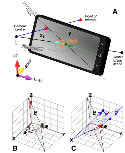
Three-dimensional reconstruction via SfM-MVS photogrammetry is based upon the collinearity equation (Fig. 1A), which defines the intersection between (1) the ray joining the camera’s optical center (hereinafter named camera position) and a given point in the object space and (2) a plane (i.e., the photo plane) lying at a given distance (i.e., focal length) from the camera position. The two-dimensional coordinates of the point of intersection on the photo plane (xi, yi), which represent the input for SfM-MVS photogrammetry reconstruction, depend upon (Fig. 1A; Table 1): (1) the camera position and the

Roll

Nort

h

Up

East

Camera centre Point of interest Center of the scene

Focal length

Focal length

ξ

y

i

x

i

Horizontal

axis

ρ

A

B

C

X

Y

Z

X

Y

Z

Figure 1. Pinhole camera model and camera rotation procedure. (A) The smartphone photo coor-dinate system in its relationships within a geographic coorcoor-dinate system, with the position and orientation of photos and points included in the scene. Notice that the camera center and focal length are shown outside the phone for sake of simplicity. ξ is the unit vector defining the cam-era view direction; ρ is the unit vector orthogonal to the camera view direction and containing the long axis of the photo; roll is the angle between the horizontal plane and the long axis of the photo, measured along the photo plane; xi and yi provide the coordinates of a point in the

photo plane along the long and short axes of the photo. (B) Rotation axis between the two unit vectors A and B. All of the rotation axes that let A become B lay on the plane g. Such a plane passes through the origin and is orthogonal to the J vector that joins A and B. The red line and dot display a rotation axis, and the red arrowed line the associated rotation pathway. (C) When two vector pairs are considered (A-B and A′-B′), the intersection between the g and g′ planes provides the rotation axis that allows simultaneous rotation of the two vector pairs. point location; (2) the orientation of the photo plane (the photo view direction), defined by the photo plane–normal unit vector ξ (the camera attitude); (3) the distance between the camera’s optical center and the photo plane (i.e., the focal length); and (4) the reference system within the photo plane, defined by the roll angle, which measures in the photo plane the angle between the hori-zontal and the long axis of the photo (defined by the unit vector ρ). Solving the collinearity equation for different photos provides the 3-D coordinates of each point detected in two or more photos. However, the full solution requires cam-era pose information (i.e., the camcam-era’s extrinsic parameters). When this infor-mation is unknown, the collinearity equation can be solved using an arbitrary 3-D reference frame, with the resultant 3-D reconstruction being output as an unreferenced point cloud. In order to georeference the scene, a further simi-larity transform (roto-translation, uniform scale) must be performed, which re-quires the known position of at least three non-collinear cameras (e.g., Turner et al., 2014) or ground control points (e.g., Carrivick et al., 2016). Conversely, deriving scaling factors requires knowing the distance between only two key points within both the real-world and arbitrary reference frames, which can be achieved with varying degrees of accuracy using rudimentary tools, such as laser distance meters in the case of small outcrops, or by measuring the dis-tance between two objects on orthophotos for larger (i.e., hundreds of meters wide) exposures. Translation is not always required in geoscience applications, especially where only the relative orientations of geologic structures (e.g., faults, fractures, bedding planes) are required (Tavani et al., 2014). Assuming that the model is accurately scaled and rotated, a coarse georegistration can be achieved by matching a single point in the arbitrary coordinate frame to the equivalent location manually identified from georeferenced remote sensing imagery and/or digital terrain models (e.g., within Google Earth).

It is clear from the above discussion that orienting the model poses the greatest challenge when attempting to spatially rectify 3-D reconstructions of real-world scenes. In practice, orienting a 3-D model is typically achieved by multiplying the 3-D coordinates of each point with a 3 × 3 rotation matrix (i.e., by rotating the model around an axis of a given rotation angle). Determining the rotation matrix requires the known locations of at least three non- collinear

Notes Plunge is positive looking downward rotation: trend Photo X Y Z Trend Plunge 20190208_094157.jpg 12.55786 41.85188 0 0 239 -4.6 20190208_094212.jpg 12.55791 41.85184 0 0.0200285 260 -3.2 20190208_094223.jpg 12.55794 41.85181 0 0.037106969 231 -2.6 20190208_094236.jpg 12.55799 41.85177 -1E-06 0.057728991 214 -3.4 20190208_094248.jpg 12.55803 41.85173 0 0.078655685 240 -1.1 20190208_094301.jpg 12.55807 41.85169 0 0.099047756 230 -1.7 20190208_094313.jpg 12.55812 41.85165 0 0.120230982 219 -1.9 20190208_094327.jpg 12.55816 41.85161 -2E-06 0.139727459 252 -3.5 20190208_094335.jpg 12.55819 41.85158 -2E-06 0.153048087 226 -3.1 20190208_094345.jpg 12.55822 41.85155 -2E-06 0.167855165 223 -2.9 20190208_094405.jpg 12.55824 41.85153 -2E-06 0.178834289 215 -3.4 20190208_094413.jpg 12.55828 41.8515 0 0.193893884 249 -2.7 20190208_094421.jpg 12.5583 41.85147 0.000001 0.206310896 223 -2.1 20190208_094429.jpg 12.55833 41.85145 0.000001 0.219047558 212 -1.6 20190208_094438.jpg 12.55837 41.85143 0 0.234482787 244 -2.6 20190208_094449.jpg 12.55841 41.85139 0 0.252812655 228 -2.3 20190208_094501.jpg 12.55847 41.85136 -1E-06 0.274821964 219 -3.1 20190208_094510.jpg 12.55852 41.85133 -1E-06 0.294220285 233 -1.8 20190208_094521.jpg 12.55857 41.85129 -2E-06 0.315167163 221 -3.6 20190208_094531.jpg 12.55862 41.85126 -2E-06 0.338379097 203 -3.3 20190208_094544.jpg 12.55868 41.85122 0.000001 0.360591845 246 -1.3 20190208_094555.jpg 12.55874 41.85119 0.000003 0.383421551 222 -1.3 20190208_094609.jpg 12.5588 41.85116 -2E-06 0.406794712 215 -2.2 20190208_094619.jpg 12.55885 41.85115 0.000006 0.423692538 251 -2 20190208_094634.jpg 12.5589 41.85111 -3E-06 0.445691666 222 -2.4 20190208_094648.jpg 12.55893 41.85105 0.000005 0.464587622 202 -3 20190208_094700.jpg 12.55894 41.85099 0.000006 0.48148111 250 -1.4 20190208_094711.jpg 12.55898 41.85094 0.000007 0.50206641 217 -3.2 20190208_094726.jpg 12.55904 41.85091 -2E-06 0.524830901 202 -2 20190208_094736.jpg 12.55909 41.85088 0.000006 0.544251562 218 -2 20190208_094746.jpg 12.55914 41.85085 0.000004 0.564942689 252 -2.8 20190208_094758.jpg 12.5592 41.85079 -3E-06 0.595074868 225 -2.9 20190208_094808.jpg 12.55926 41.85075 -5E-06 0.617290452 203 -1.3 20190208_094819.jpg 12.55929 41.85073 -2E-06 0.632267917 250 -1.6 20190208_094830.jpg 12.55934 41.85067 -1E-06 0.654963971 236 -2 20190208_094840.jpg 12.55936 41.85062 -2E-06 0.672992015 229 -2.4 20190208_094853.jpg 12.55939 41.85057 -3E-06 0.693877447 267 -1.3 20190208_094904.jpg 12.55943 41.85051 -3E-06 0.715027212 244 -1.7 20190208_094914.jpg 12.55946 41.85046 -3E-06 0.736651217 231 -1.1 20190208_094925.jpg 12.55951 41.85041 -2E-06 0.759125198 267 -1.2 20190208_094935.jpg 12.55955 41.85036 -4E-06 0.781610609 216 -1 20190208_094946.jpg 12.55959 41.85031 -3E-06 0.803875324 257 -1.6 20190208_094959.jpg 12.55963 41.85027 -3E-06 0.824503809 277 -2.7 20190208_095009.jpg 12.55969 41.85024 -5E-06 0.844216499 236 -2 20190208_095018.jpg 12.55973 41.85019 -5E-06 0.867218554 213 -1.3 20190208_095028.jpg 12.55978 41.85015 -4E-06 0.889191861 267 -1.9 20190208_095039.jpg 12.55983 41.8501 -4E-06 0.912427823 234 -2 Position along strip

Estimated position Measured ξ

points, both in the arbitrary reference system and in the target reference frame. In the field, this ostensibly trivial problem is exacerbated by the poor portability and/or high cost of local and global positioning systems capable of achieving survey-grade measurement accuracies. Indeed, recognizing the position of three non-collinear points in 3-D virtual scenes is relatively simple, whereas determining their positions in the north-east-up reference system re-quires centimeter to sub-centimeter accuracy, achievable with a total station or RTK-DGNSS receivers.

The alternative workflow for orienting models explored in this work con-sists of taking attitude data tagged to smartphone images, rather than the posi-tion of ground control points, for determining the 3-D model’s rotaposi-tional trans-form. In summary, our procedure consists of three simple steps: (1) acquire smartphone photos with the AngleCam app for Android, a software application which records and stores camera attitude data associated with individual pho-tographs; (2) build a model using the smartphone photos and extract the esti-mated unit vector ξ and roll angle (and the associated unit vector ρ; Fig. 1A) of the photos as defined in the arbitrary reference system; and (3) determine the rotation matrix using the measured and estimated values of ξ and roll.

The 3-D models presented in this work were constructed using Agisoft PhotoScan software (Verhoeven, 2011; Plets et al., 2012), version 1.4.4, Pro-fessional Edition, a commercially available SfM-MVS photogrammetric tool chain. Photo-alignment in PhotoScan allows for the estimated direction of photos (estimated ξ and estimated ρ) to be derived, whereas measured ξ and measured roll angle are provided by the AngleCam app (the roll angle is then transformed into the measured ρ). The rule adopted herein is that the trend of ξ is the direction of view with respect to north, and the plunge for both ξ and ρ is positive looking downward. The trend of the ρ unit vector is taken, looking in the same direction and sense as the ξ direction, on the right side of the ρ direction.

The four unit vectors (i.e., measured ξ, estimated ξ, measured ρ, and es-timated ρ) are required by the presented workflow to orient a virtual outcrop

model (their value for the photos for the five models presented herein are pro-vided in the Supplementary Material1_{). Specifically, the rotation axis (Rax) and} rotation angle (Ran) of each model are derived by adopting a procedure of minimization of the residual sum of squares (RSS). Given two unit vectors A and B, all of the rotation axes that permit the transformation of A to B lay on the plane g orthogonal to the vector joining A and B (hereinafter named vector J) and passing through the origin of the coordinate frame (Fig. 1B). If a second vector pair (A′ and B′) is added to the system, along with its J′ vector and g′ plane (Fig. 1C), the intersection between g and g′ provides the rotation axis that allows simultaneous rotation of the two vector pairs. For each unit vector pair (i.e., measured and estimated ξ and measured and estimated ρ), the Jξ and Jρ vectors (which join the measured and estimated unit vectors; see Table 1) are computed, as well as the planes perpendicular to these vectors. For each model, the optimal rotation axis is provided by the maximum inter-section of these planes. The plane normal vectors (J vectors) are transformed into a second-order symmetric tensor (e.g., Whitaker and Engelder, 2005): the eigenvector corresponding to minimum eigenvalue is the direction of mini-mum concentration of J, which is the direction of maximini-mum concentration of intersections between planes (i.e., the optimal rotation axis, Rax). Having de-fined the axis of rotation, estimated ξ and ρ of each photo is rotated around

Rax using 0.1° increments. Using the entire photographic data set, the RSS

be-tween the rotated ξ and ρ and the measured ξ and ρ of each photo is computed. The angle generating the minimum RSS is taken as the Ran. This procedure is implemented in OpenPlot software (Tavani et al., 2011).

MODEL BUILDING

Two “test” and three “field” models were constructed using Agisoft Photo-Scan software (e.g., Verhoeven, 2011; Plets et al., 2012) to evaluate the feasibil-ity and effectiveness of the procedure.

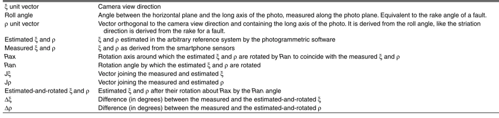
TABLE 1. PARAMETER NOTATION

ξ unit vector Camera view direction

Roll angle Angle between the horizontal plane and the long axis of the photo, measured along the photo plane. Equivalent to the rake angle of a fault.

ρ unit vector Vector orthogonal to the camera view direction and containing the long axis of the photo. It is derived from the roll angle, like the striation

direction is derived from the rake for a fault.

Estimated ξ and ρ ξ and ρ estimated in the arbitrary reference system by the photogrammetric software

Measured ξ and ρ ξ and ρ as derived from the smartphone sensors

Rax Rotation axis around which the estimated ξ and ρ are rotated by Ran to coincide with the measured ξ and ρ

Ran Rotation angle by which the estimated ξ and ρ are rotated

Jξ Vector joining the measured and estimated ξ

Jρ Vector joining the measured and estimated ρ

Estimated-and-rotated ξand ρ Estimated ξ and ρ after their rotation about Rax by the Ran angle

∆ξ Difference (in degrees) between the measured and the estimated-and-rotated ξ

∆ρ Difference (in degrees) between the measured and the estimated-and-rotated ρ

1_{Supplemental Material. Camera orientation}

in-formation for the models presented in this work.

Please visit https://doi.org/10.1130/GES02167.S1

or access the full-text article on www.gsapubs.org to view the Supplemental Material.

Test Models

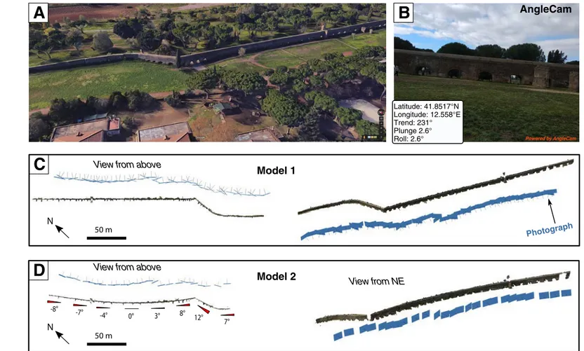
Two test models of a 200-m-long segment of the “Acquedotto Felice” in the Park of Aqueducts in the city of Rome (Italy) were constructed using 12 Mpx (megapixel) images, captured using a Xiaomi MiA1 smartphone (Fig. 2A). Angle-Cam, developed for the Android mobile operating system (http://anglecam.derekr .com), was used to obtain the camera attitude associated which each survey photo in the form of trend, plunge, and roll angle (Fig. 2B). First, the handset was set to airplane mode to reduce electromagnetic interference between the

mag-netometer and the smartphone’s computing hardware (the reader should note that recent findings indicate that having the airplane mode off does not signifi-cantly affect orientation measurements; Novakova and Pavlis, 2017). Moreover, the handset’s integrated compass and accelerometer were both calibrated using the provided calibration tool. A 51-photograph data set was acquired at a distance of ~30 m from the aqueduct. Photos were acquired approximately perpendicular to the aqueduct, and at two opposing oblique angles (~50°) to its strike.

The first test model was constructed using the entire photo data set (model 1; Fig. 2C) and resulted in a point cloud of nearly 4 × 106 _{points. The second}

A

B

AngleCam

C

D

View from above

View from above

View from NE

-8° _-7° -4° 0° 3° 8° 12° 7° 50 m

N

50 m

N

Model 1

Model 2

Photograph Latitude: 41.8517°N Longitude: 12.558°E Trend: 231° Plunge 2.6° Roll: 2.6°

Figure 2. Workflow for construction of test models. (A) Google Maps three-dimensional view of the Acquedotto Felice (Rome, Italy). (B) Example of photo captured using the AngleCam smartphone app, with the location and orientation of the camera shown in the lower left box. (C,D) Orthographic view from above and from the northeast of model 1 (C) and model 2 (D) built in Agisoft PhotoScan software. The blue lines (models on the left) and planes (models on the right) represent the photographs used to build the models. The angular difference of the aqueduct wall strike between the two models at different locations is reported in model 2. These values provide an indication of the distortion in model 2.

model consisted of a point cloud of 3 × 106 _{vertices and was constructed only} using photographs that were approximately perpendicular to the aqueduct, exhibiting poor image overlap. The survey regimen of the latter data set was designed to enhance the doming effect of the reconstructed scene in order to produce an intentionally deformed model (model 2; Fig. 2D). The four unit vectors of each photo (i.e., estimated and measured ξ and estimated and mea-sured ρ) were used to determine the rotation matrix for each model. After ro-tating the estimated ξ and ρ, we obtain the estimated-and-rotated ξ and ρ of each photo.

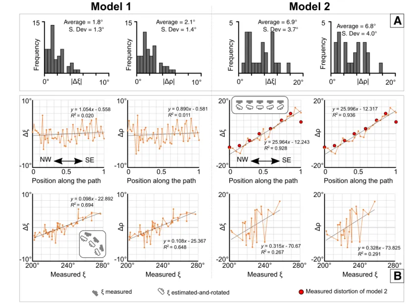
Ideally, when measurement errors and model distortions do not occur, the estimated-and-rotated ξ and ρ for each photo should exactly coincide with the measured ξ and ρ. Therefore, differences between measured and estimat-ed-and-rotated parameters provide an indirect estimation of model quality. Accordingly, the angular difference between the measured and transformed ξ and between the measured and transformed ρ, from hereon named Dξ and Dρ, respectively, were computed. The average of the absolute values of both pa-rameters is nearly 2° for model 1, whereas it is ~7° for model 2 (i.e., the model with induced geometric distortion) (Fig. 3A). In Figure 3, we also plot Dξ and Dρ versus the position of photograph along the survey path and the measured photo direction (measured ξ) (Fig. 3B). These plots evidence a remarkable dif-ference between the two models.

In model 1, both Dξ and Dρ show poor correlation with the position along the survey path, these parameters being nearly -0.5° and 0.5° at the two ends of the survey path respectively. Moreover, for model 1, the line of best fit has a low R2 _{(<0.02), indicating low residual error between AngleCam-measured and} transformed SfM-estimated orientation of cameras. In model 1, both Dξ and Dρ correlate with the measured ξ, with the R2 _{of the linear fit being >0.6. The} mea-sured ξ ranges between 200° and 280° and, in this 80°-wide interval, Dξ and Dρ pass from nearly -4° to 4°, with a slope of the line of best fit being ~0.1°. For model 2, both Dξ and Dρ increase with increasing (measured) ξ, with a slope of the line of best fit being 0.3°, thus the difference between the measured and the estimate-and-rotated directions is more sensitive to the photo direction. However, R2 _{is <0.3 for model 2. Although model 2 is more sensitive to photo} direction than model 1, the distortions are still mostly dependent on survey position. Indeed, Dξ and Dρ correlate strongly with the position along the sur-vey path, with a R2 _{of the best fit line of 0.9 and a slope of 26° (implying values} of about -13° and 13° at the two ends of the survey path, respectively). Also, the linear regression of Dξ and Dρ versus position along the survey path shows a remarkable fit with the measured distortion of model 2 (indicated with red circular markers in Fig. 3B). In detail, the measured distortion represents the angular difference between the reconstructed and real-world scene. A similar analysis has not been conducted for model 1, as the distortion for this model is ostensibly <0.5° along the entire survey path, and the red markers in Figure 3B would all lie at y = 0.

In summary: (1) Dξ and Dρ have similar trends in all plots; (2) the “distorted” model (model 2) has higher average values for the absolute value of Dξ and Dρ, higher slopes of the best-fit linear regressions for the Dξ and Dρ versus

mea-sured ξ plots, and higher slopes of the best-fit linear regression for the plots of Dξ and Dρ versus position along the survey path; (3) the graph relating Dξ and Dρ to the position along the survey path (which is displayed only for model 2) overlaps the measured distortions along the model.

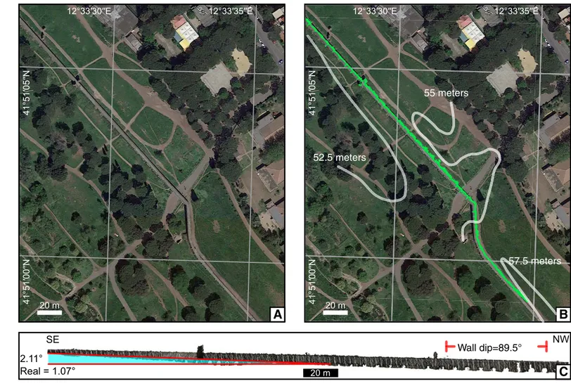
In Figure 4, we show how well model 1 conforms to the geometry of the mapped scene. Figure 4A displays an orthophoto of the area of the Acquedotto Felice. Figure 4B displays the same orthophoto with topographic contours, and with the reconstructed 3-D model (green markers) seen in orthographic nadir view. Note that the reconstructed model shows excellent agreement with the northeasterly facing exterior wall of the Acquedotto Felice, with an angular de-viation of <0.5°. This value becomes ~2.5° when considering the magnetic dec-lination of the area (~3° east). Figure 4C displays the frontal view of the model using orthographic projection, with the slope computed between two points of known altitude (topographic contours displayed in Fig. 4B). The difference between the computed (2.11°) and real (1.07°) slope is close to 1°. Finally, using OpenPlot (Tavani et al., 2011), we computed the dip (i.e., the measure of how vertical the aqueduct wall is) of a 60-m-wide segment of the aqueduct, which is 89.5° (only the near-vertical portions of the aqueduct were used for this pur-pose) and serves to quantify the angular difference around a third axis nearly orthogonal to the previous two (i.e., the vertical axis and the axis parallel to the view direction of Fig. 4C). In summary, in order to fully fit the real geometry of the aqueduct, the reconstructed model 1 must be rotated ~2° around a vertical axis and ~1° about two mutually perpendicular horizontal axes.

Field Models

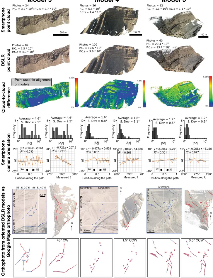
Field models consist of three models of geological exposures from the Oman Mountains (also known as Al-Hajar Mountains; eastern Arabian Penin-sula), where hundred-meter-wide poorly vegetated exposures were mapped using a Xiaomi MiA1 smartphone (12 Mpx; sensor size, 5.11 × 3.84 mm; focal length [35 mm equivalent], 26 mm) and a Nikon D5300 DSLR camera (24 Mpx; sensor size, 23.5 × 15.6 mm; focal length [35 mm equivalent], 27 mm). For model 3, no compass calibration was carried out before image capture, with airplane mode switched off during image acquisition. Conversely, for models 4 and 5, the smartphone was set to airplane mode and compass calibration was performed prior to photo acquisition.

Models of the three exposures were independently built from the smart-phone and DSLR data sets using Agisoft PhotoScan (Fig. 5). We attempted to merge the two photographic data sets (i.e., smartphone and DSLR) within a single model. However, this led to point clouds with lower vertex densities when compared with models generated exclusively from DSLR images. Once constructed, the point clouds were imported into CloudCompare (https://www .danielgm.net/cc/), an open-source point cloud processing and analysis soft-ware tool, where the smartphone and DSLR models were manually aligned us-ing a minimum of six keypoints. For each model, and for the overlappus-ing area between smartphone- and DSLR-derived models, the vertex-to-vertex distance

Model 1

15

0°

|Δξ|

10°

Frequenc

y

5

0°

|Δξ|

20°

Frequency

Average = 1.8° S. Dev = 1.3° Average = 6.9° S. Dev = 3.7°

15

0°

|Δρ|

10°

Frequenc

y

5

0°

|Δρ|

20°

Frequency

Average = 2.1° S. Dev = 1.4° Average = 6.8° S. Dev = 4.0°

Model 2

0.5

10°

-10°

0

1

y = 1.054x - 0.558 R2 _{= 0.020}

Δξ

Position along the path

0.5

10°

-10°

0

1

y = 0.890x - 0.581

R2 _{= 0.011}

Position along the path

Δρ

NW

SE

240°

10°

-10°

200°

280°

Δξ

Measured ξ

y = 0.098x - 22.892 R2 _{= 0.694}

240°

10°

-10°

200°

280°

Δρ

Measured ξ

y = 0.108x - 25.367 R2 _{= 0.648}

0.5

20°

-20°

0

1

y = 25.964x - 12.243 R2 _{= 0.928}

Δξ

Position along the path

0.5

20°

-20°

0

1

y = 25.996x - 12.317

R2 _{= 0.936}

Position along the path

Δρ

NW

SE

240°

20°

-20°

200°

280°

Δξ

Measured ξ

y = 0.315x - 70.67 R2 _{= 0.267}

20°

-20°

Δρ

Measured ξ

y = 0.328x - 73.825 R2 _{= 0.291}

-ξ measured ξ estimated-and-rotated Measured distortion of model 2

A

-B

240°

200°

280°

Figure 3. Photo orientation and reconstruction quality for the test models shown in Figure 2. (A) Frequency distribution of the absolute difference between the measured and estimat-ed-and-rotated photo orientation parameters (i.e., Dξ = [measured ξ] – [estimated-and-rotated ξ] and D ρ = [measured ρ] – [estimated-and-rotated ρ], being ξ the unit vector defining the camera view direction and ρ the unit vector orthogonal to the camera view direction and containing the long axis of the photo). S. Dev—standard deviation. (B) Plots relating Dξ and D ρ to the position along the survey path (values are normalized between 0 and 1) and the measured ξ. The red circular markers in the plots of model 2 indicate the angular difference between the reconstructed and real wall, as shown in Figure 2D. The insets with white and gray cameras serve to illustrate in map view the distortion in camera orientation as derived from the corresponding graph.

between compared models was computed. Deviations between the trans-formed models are displayed in Figure 5 as percentage of the exposure width. For all models, this difference is below ~0.1%–0.2%. It is worth noting that such a value incorporates both geometric differences between the models and di-vergence related to the alignment procedure. An optimized alignment could potentially reduce the calculated disparities between the compared models. However, at this stage our main purpose is to establish the equivalence of the

DSLR and smartphone models in order to demonstrate the reproducibility of results from each data-capture modality.

For the reorientation of smartphone models, the same procedure described for test models 1 and 2 was repeated. The measured and estimated camera ori-entation parameters were used to derive the rotation matrix and values of Dξ and Dρ for each photo. The average value of the modulus of Dξ and Dρ for models 4 and 5 is extremely low (<2°), while for model 3 it is 4.6° for both parameters. Due

41°51′05′′N 20 m

A

41°51′00′′N 12°33′30′′E 12°33′35′′E 41°51′05′′ N 20 m

B

41°5 1′0 0′′ N 12°33′30′′E 12°33′35′′E 41 °5 1′ 05 ′′N 1°5 1′ 00 ′′N

55 meters

57.5 meters

55

52.5 meters

20 m

C

2.11°

Real = 1.07°

SE

NW

Wall dip=89.5°

Figure 4. Comparison between model and the real world scene for test models shown in Figure 2. (A) Google Maps orthophoto of the Acquedotto Felice area (Rome, Italy). (B) Google Maps orthophoto of the Acquedotto Felice area with topographic contours (every 2.5 meters) and overlay of model 1 (green points). (C) Frontal view (orthographic mode) of model 1, with slope at the base of the structure computed between two points in the model (2.11°) and in the real world (1.07°, computed using the topographic contours shown in B). For the north-western portion of the aqueduct, the dip (i.e., the measure of how vertical the aqueduct wall is) of the near-vertical portion of the wall, as extracted from the model, is indicated (89.5°).

|

V olume 15

|

Number 6 Tavani et al.

|

Smar tphone: An alter

native to GCPs for orienting vir

tual outcr op models

Research Paper

Or

thophoto fr

om oriented DSLR models vs

Google Mape or

thophoto

Figure 5. Field models (Oman Mountains, eastern Arabian Peninsula). Diagrams for each model (column) are described from top to bottom. (Rows 1–3) Frontal view of the smartphone- (1) and digital single-lens reflex (DSLR) (2) camera–based models, and the distance between them (computed as a percentage of the model width) (3). For both models, the number of photos is indicated, along with the number of points in the entire point cloud (P.C.) and in the overlapping area between the two models (P.C.s). Homologous points in the DSLR and smartphone models used to align the two models are also indicated. (Row 4) Frequency distribution of the modulus of Dξ and D ρ (Dξ = [measured ξ] – [estimated-and-rotated ξ] and D ρ = [measured ρ] – [estimated-and-rotated ρ], being ξ the unit vector defining the camera view direction and ρ the unit vector orthogonal to the camera view direction and containing the long axis of the photo). (Row 5) Graphs relating Dξ to the position along the survey path (values are normalized between 0 and 1) and the measured ξ. (Row 6) Orthophotos of the models after their alignment (on the right) and orthophotos of the same area from Google Maps (on the

to the similar behavior of Dξ and Dρ, as seen in Figure 3, for these three field mod-els, we plot only Dξ versus the position of the photo along the survey path and the measured photo direction ξ (Fig. 5). For all models, Dξ versus position along the survey path is characterized by linear regressions having a slope <3.2 and R2 <0.31, which means that the maximum distortion between the edges of the mod-els is ~3°, indicating that the doming effect is negligible (especially for modmod-els 4 and 5). For models 4 and 5, the slope of the best-fit linear regression between Dξ and measured ξ is <0.06, whereas for model 1 it is 0.7. The derived rotation matrix was also used to rotate the three smartphone models in CloudCompare, obtain-ing oriented smartphone models. Oriented DSLR models (with higher resolution and improved noise characteristics) were then obtained by alignment to these previously oriented smartphone models.

Oriented DSLR-derived models, seen from above in orthographic projec-tion mode (here termed DSLR orthophotos), are shown in Figure 5, along with the same area as seen in orthophotos from Google Maps. Some key features (e.g., vertical cliffs, large boulders, buildings, trees) have been traced on both Google Maps and DSLR orthophotos to scale the DSLR model and later esti-mate the angular difference between the oriented DSLR models and georef-erenced aerial photography. Rotations around the vertical axis of <2° had to be applied to models 4 and 5 to match Google’s orthophotos (which remained <2° when considering the present-day magnetic declination of the area, 1.5° east). In contrast, model 3 is strongly misoriented, as indicated by a rotation >40° being required to match features observed in the DSLR orthophoto and Google’s orthophoto. It should be noted that user errors introduced during the tracing procedure do not appear to significantly affect these values: consider-ing the resolution of both Google’s orthophotos and our DSLR models (~1 m), errors resulting from the manual picking of objects is on the order of a couple of meters, which for the studied 0.5-km-wide region of interest, translates into maximum admissible angular errors of <0.3°.

DISCUSSION AND BEST PRACTICE

The potential application of orientation of photographs, rather than the position of known features, to accurately orient SfM-MVS photogrammetry– derived models was recently suggested by Fleming and Pavlis (2018). Here, we have expanded upon this proposition by using the orientation parameters associated with smartphone-captured imagery to produce accurately oriented intermediate-resolution models. These were later used to successfully orient higher- resolution DSLR derived models. We have also computed the difference between measured and estimated camera orientation parameters, namely Dξ and Dρ, which provides an indirect indication of the quality of the reconstruction.

Both systematic and random errors occur in the smartphone measure-ments (Allmendinger et al., 2017), and SfM-MVS models always include distor-tions and range-error artifacts (Carrivick et al., 2016). Systematic measurement errors for smartphones are undetectable without an external control tool (e.g., the Google Maps orthophotos used in Figs. 3 and 5). Conversely, random

mea-surement errors in the smartphone camera attitude or in the extrinsic camera calibration are expected to produce a mismatch between the measured and estimated camera orientation. Anecdotally, our case study results are in agree-ment with the above, whereby lower values of Dξ and Dρ correspond to models with null observable global geometric distortions. The average values of Dξ and Dρ for models 1, 4, and 5 is ~2°, and, as observed in Figure 4, this corresponds to a mismatch between the reconstructed model and the real-world scene of ~2°. The two models with distortions (i.e., models 2 and 3) are characterized by average values of Dξ and Dρ ranging between 4.6° and 7°. The source of error for these two models is different, as depicted by plots of Dξ versus position along the survey path and measured ξ. Figures 4 and 5 show that for models 1, 3, 4, and 5, no remarkable doming effect occurs. For all of these models, Dξ versus position along the survey path graph is characterized by a best-fit linear regression with low R2 _{(<0.31) and low slope (ranging between -0.5 and} 3.1). Conversely, for model 2, where we induced a doming effect, the slope value is ~26 and the value of Dξ is essentially controlled by the position of the photograph along the survey path, as evidenced by the high R2 _{(0.93). Also, it} is worth noting that in this graph for model 2, the Dξ overlaps the measured distortion of the model. In agreement, Dξ versus position along the survey path successfully describes the model’s geometric distortion associated with the doming effect. The source of error for model 3 is instead associated with errors in the smartphone inclinometer and magnetometer measurement, which we attribute the correct operating procedure not being applied prior to and during data capture (note that the compass and the accelerometer were not calibrated and airplane mode was not activated before photo acquisition for this model). This results in a model registration based upon unreliable orientation data. This is in line with previous work on the use of smartphones as measurement tools (Allmendinger et al., 2017; Novakova and Pavlis, 2017), indicating that recalibration of sensors before acquiring images for building a VOM should be practiced to avoid orientation measurement errors. The measurement errors in model 3 are manifested not only by the high average value of the modulus of Dξ and Dρ, but also by plots of Dξ versus measured ξ. Notably, the slope of the linear regression of Dξ versus measured ξ for model 3 is 0.9, whereas it is <0.1 for the optimized models (i.e., models 1, 4, and 5). To summarize, Dξ provides two additional parameters, which are the slopes of the best-fit lines of (1) Dξ versus measured ξ and (2) Dξ versus position along the survey path. These two derivative parameters serve to define the quality of a model and, in the case presented here, to understand the source of the model’s distortion. However, the Dξ parameter can also be used independently to discriminate be-tween geometrically accurate and distorted models: anecdotally, we find that average values of Dξ <2° provides indication of models reconstructed with a high degree of geometric fidelity.

A final note concerns the accuracy of smartphone sensors (i.e., magneto-meter and acceleromagneto-meter), which forms the most conspicuous potential source of error within the presented workflow. We have provided strong evidence sup-porting the high degree of accuracy of smartphone-based attitudinal measure-ments (i.e., errors <1° for the test model 1). This is not surprising, as smartphones

have previously been successfully employed as a compass during many field campaigns. During these campaigns, comparison with data acquired by means of a Silva compass constantly indicates that errors are typically <2°. To quantify these discrepancies more accurately, we suggest that users conduct stability and accuracy analyses before employing specific smartphones for orientation data collection, as individual models of handsets may have error characteristics that are different from those of the model used within this study.

CONCLUSIONS

In this work, we have proposed a workflow to produce properly oriented 3-D models by means of terrestrial SfM-MVS photogrammetry, which involves the use of smartphone photos. Our results are encouraging and indicate that high-precision registrations of 3-D reconstructed scenes can be achieved in a few simple steps. Orientation parameters of smartphone photos can be used with the twofold purpose of orienting high-resolution DSLR models and pro-viding input for estimating model quality. We have individuated three param-eters defining the quality of a model: (1) the average value of the modulus of Dξ and Dρ, which, roughly, is of 2° or less for high-quality models with null geometric distortion, and >4 for models having noticeable distortion; (2) the slope of the best-fit line of a plot of Dξ versus position along the survey path, which in high-quality models is <3 (or <-3); and (3) the slope of the best-fit line of a plot of Dξ versus measured ξ, which in high-quality models is ≤0.1. ACKNOWLEDGMENTS

Comments by Reuben Hansman, Zachariah Fleming, and Terry Pavlis greatly helped us to improve the original version of the paper.

REFERENCES CITED

Allmendinger, R.W., Siron, C.R., and Scott, C.P., 2017, Structural data collection with mobile devices: Accuracy, redundancy, and best practices: Journal of Structural Geology, v. 102, p. 98–112, https://doi.org/10.1016/j.jsg.2017.07.011.

Bemis, S.P., Micklethwaite, S., Turner, D., James, M.R., Akciz, S., Thiele, S.T., and Bangash, H.A., 2014, Ground-based and UAV-based photogrammetry: A multi-scale, high-resolution mapping tool for structural geology and paleoseismology: Journal of Structural Geology, v. 69, p. 163–178, https://doi.org/10.1016/j.jsg.2014.10.007.

Bisdom, K., Bertotti, G., and Nick, H.M., 2016, The impact of different aperture distribution models and critical stress criteria on equivalent permeability in fractured rocks: Journal of Geophysical Research: Solid Earth, v. 121, p. 4045–4063, https://doi.org/10.1002/2015JB012657. Bistacchi, A., Balsamo, F., Storti, F., Mozafari, M., Swennen, R., Solum, J., Tueckmantel, C., and

Taberner, C., 2015, Photogrammetric digital outcrop reconstruction, visualization with textured surfaces, and three-dimensional structural analysis and modeling: Innovative methodologies applied to fault-related dolomitization (Vajont Limestone, Southern Alps, Italy): Geosphere, v. 11, p. 2031–2048, https://doi.org/10.1130/GES01005.1.

Carrivick, J.L., Smith, M.W., and Quincey, D.J., 2016, Structure from Motion in the Geosciences: Chichester, UK, Wiley-Blackwell, https://doi.org/10.1002/9781118895818.

Corradetti, A., McCaffrey, K., De Paola, N., and Tavani, S., 2017, Evaluating roughness scaling properties of natural active fault surfaces by means of multi-view photogrammetry: Tectonophysics, v. 717, p. 599–606, https://doi.org/10.1016/j.tecto.2017.08.023.

Favalli, M., Fornaciai, A., Isola, I., Tarquini, S., and Nannipieri, L., 2012, Multiview 3D reconstruction in geosciences: Computers & Geosciences, v. 44, p. 168–176, https://doi.org/10.1016/j.cageo .2011.09.012.

Fleming, Z.D., and Pavlis, T.L., 2018, An orientation based correction method for SfM-MVS point clouds—Implications for field geology: Journal of Structural Geology, v. 113, p. 76–89, https:// doi.org/10.1016/j.jsg.2018.05.014.

Hansman, R.J., and Ring, U., 2019, Workflow: From photo-based 3-D reconstruction of remotely piloted aircraft images to a 3-D geological model: Geosphere, v. 15, p. 1393–1408, https://doi .org/10.1130/GES02031.1.

Harwin, S., and Lucieer, A., 2012, Assessing the accuracy of georeferenced point clouds produced via multi-view stereopsis from unmanned aerial vehicle (UAV) imagery: Remote Sensing, v. 4, p. 1573–1599, https://doi.org/10.3390/rs4061573.

James, M.R., and Robson, S., 2014, Mitigating systematic error in topographic models derived from UAV and ground-based image networks: Earth Surface Processes and Landforms, v. 39, p. 1413–1420, https://doi.org/10.1002/esp.3609.

James, M.R., Robson, S., d’Oleire-Oltmanns, S., and Niethammer, U., 2017, Optimising UAV topographic surveys processed with structure-from-motion: Ground control quality, quantity and bundle adjustment: Geomorphology, v. 280, p. 51–66, https://doi.org/10.1016/j .geomorph.2016.11.021.

Javernick, L., Brasington, J., and Caruso, B., 2014, Modeling the topography of shallow braided rivers using Structure-from-Motion photogrammetry: Geomorphology, v. 213, p. 166–182, https://doi.org/10.1016/j.geomorph.2014.01.006.

Martínez-Carricondo, P., Agüera-Vega, F., Carvajal-Ramírez, F., Mesas-Carrascosa, F.-J., García-Ferrer, A., and Pérez-Porras, F.-J., 2018, Assessment of UAV-photogrammetric mapping accuracy based on variation of ground control points: International Journal of Applied Earth Observation and Geoinformation, v. 72, p. 1–10, https://doi.org/10.1016/j.jag.2018.05.015. Nocerino, E., Menna, F., and Remondino, F., 2014, Accuracy of typical photogrammetric networks

in cultural heritage 3D modeling projects: International Archives of the Photogrammetry, Remote Sensing and Spatial Information Sciences, v. XL-5, p. 465–472, https://doi.org/10.5194/ isprsarchives-XL-5-465-2014.

Novakova, L., and Pavlis, T.L., 2017, Assessment of the precision of smart phones and tablets for measurement of planar orientations: A case study: Journal of Structural Geology, v. 97, p. 93–103, https://doi.org/10.1016/j.jsg.2017.02.015.

Plets, G., Verhoeven, G., Cheremisin, D., Plets, R., Bourgeois, J., Stichelbaut, B., and De Reu, J., 2012, The deteriorating preservation of the Altai rock art: Assessing three-dimensional image-based modelling in rock art research and management: Rock Art Research, v. 29, p. 139–156. Seers, T.D., and Hodgetts, D., 2016, Extraction of three-dimensional fracture trace maps from calibrated

image sequences: Geosphere, v. 12, p. 1323–1340, https://doi.org/10.1130/GES01276.1. Sturzenegger, M., and Stead, D., 2009, Close-range terrestrial digital photogrammetry and

terrestrial laser scanning for discontinuity characterization on rock cuts: Engineering Geology, v. 106, p. 163–182, https://doi.org/10.1016/j.enggeo.2009.03.004.

Tavani, S., Arbues, P., Snidero, M., Carrera, N., and Muñoz, J.A., 2011, Open Plot Project: An open-source toolkit for 3-D structural data analysis: Solid Earth, v. 2, p. 53–63, https://doi .org/10.5194/se-2-53-2011.

Tavani, S., Granado, P., Corradetti, A., Girundo, M., Iannace, A., Arbués, P., Muñoz, J.A., and Mazzoli, S., 2014, Building a virtual outcrop, extracting geological information from it, and sharing the results in Google Earth via OpenPlot and Photoscan: An example from the Khaviz Anticline (Iran): Computers & Geosciences, v. 63, p. 44–53, https://doi.org/10.1016/j.cageo.2013.10.013. Tavani, S., Corradetti, A., and Billi, A., 2016, High precision analysis of an embryonic extensional

fault-related fold using 3D orthorectified virtual outcrops: The viewpoint importance in structural geology: Journal of Structural Geology, v. 86, p. 200–210, https://doi.org/10.1016/j .jsg.2016.03.009.

Turner, D., Lucieer, A., and Wallace, L., 2014, Direct georeferencing of ultrahigh-resolution UAV imagery: IEEE Transactions on Geoscience and Remote Sensing, v. 52, p. 2738–2745, https:// doi.org/10.1109/TGRS.2013.2265295.

Verhoeven, G., 2011, Taking computer vision aloft—Archaeological three-dimensional reconstructions from aerial photographs with PhotoScan: Archaeological Prospection, v. 18, p. 67–73, https://doi.org/10.1002/arp.399.

Whitaker, A.E., and Engelder, T., 2005, Characterizing stress fields in the upper crust using joint orientation distributions: Journal of Structural Geology, v. 27, p. 1778–1787, https://doi.org/ 10.1016/j.jsg.2005.05.016.