Contents lists available atScienceDirect
Ecological Modelling
journal homepage:www.elsevier.com/locate/ecolmodel
Ecosystem services accounts: Valuing the actual flow of nature-based
recreation from ecosystems to people
Sara Vallecillo
a,⁎, Alessandra La Notte
a, Grazia Zulian
a, Silvia Ferrini
b,c, Joachim Maes
a aEuropean Commission – Joint Research Centre, Via Enrico Fermi, 2749 – TP 270, 21027 Ispra, ItalybDepartment of Political and International Sciences, University of Siena, Via Mattioli 10, 53100 Siena, Italy cCSERGE, School of Environmental Sciences, University of East Anglia, Norwich, United Kingdom
A R T I C L E I N F O Keywords: Service potential Service demand Daily recreation Wellbeing Monetary value Accounting tables A B S T R A C T
Natural capital accounting aims to measure changes in the stock of natural assets (i.e., soil, air, water and all living things) and to integrate the value of ecosystem services into accounting systems that will contribute to better ecosystems management. This study develops ecosystem services accounts at the European Union level, using nature-based recreation as a case study and following the current international accounting framework: System of Environmental-Economic Accounting – Experimental Ecosystem Accounting (SEEA EEA). We adapt and integrate different biophysical and socio-economic models, illustrating the workflow necessary for eco-system services accounts: from a biophysical assessment of nature-based recreation to an economic valuation and compilation of the accounting tables. The biophysical assessment of nature-based recreation is based on spatially explicit models for assessing different components of ecosystem services: potential, demand and actual flow. Deriving maps of ecosystem service potential and demand is a key step in quantifying the actual flow of the service used, which is determined by the spatial relationship (i.e., proximity in the case of natubased re-creation) between service potential and demand. The nature-based recreation accounts for 2012 show an actual flow of 40 million potential visits to ‘high-quality areas for daily recreation’, with a total value of EUR 50 billion. This constitutes an important contribution of ecosystems to people's lives that has increased by 26% since 2000. Practical examples of ecosystem services accounts, as shown in this study, are required to derive re-commendations and further develop the conceptual and methodological framework proposed by the SEEA EEA. This paper highlights the importance of using spatially explicit models for ecosystem services accounts. Mapping the different components of ecosystem services allows proper identification of the drivers of changes in the actual service flow derived from ecosystems, socio-economic systems and/or their spatial relationship. This will contribute to achieving one of the main goals of ecosystem accounts, namely measuring changes in natural capital, but it will also support decision-making that targets the enhancement of ecosystems, their services and the benefits they provide.
1. Introduction
A region's economic prosperity and wellbeing is underpinned by its natural capital. Natural capital is the world's stock of natural assets, which includes geology, soil, air, water and all living organisms. It is from this natural capital that humans derive a wide range of ecosystem services such as protection against natural disasters, climate regulation, pollination and nature-based recreation, all of which make human life possible. Natural capital accounting is a tool to measure the changes in
the stock of natural assets and to integrate the value of ecosystem services into accounting and reporting systems, which will contribute to more effective ecosystem and land management measures.
The Seventh Environment Action Programme and the Biodiversity Strategy to 2020 of the European Union (EU) include objectives to develop natural capital accounts in the EU, with a focus on ecosystems and their services. More specifically, Action 5 of the EU Biodiversity Strategy requires Member States, with the assistance of the European Commission, “to map and assess the state of ecosystems and their
https://doi.org/10.1016/j.ecolmodel.2018.09.023
Received 18 April 2018; Received in revised form 21 September 2018; Accepted 26 September 2018
Abbreviations: EB-P, ecosystem-based potential; ES, Ecosystem services; EU, European Union; LAU, Local Administrative Unit; LUT, lookup tables; MENE, Monitor
of Engagement with the Natural Environment; SBA, service benefiting area; SEEA EEA, System of integrated Environmental-Economic Accounting – Experimental Ecosystem Accounts; SNA, System of National Accounts; SPA, service providing area; TCM, travel cost method; UN, United Nations
⁎Corresponding author.
E-mail address:[email protected](S. Vallecillo).
0304-3800/ © 2018 The Authors. Published by Elsevier B.V. This is an open access article under the CC BY-NC-ND license (http://creativecommons.org/licenses/BY-NC-ND/4.0/).
services. They must also assess the economic value of such services, and promote the integration of these values into accounting and reporting systems at the EU and national level by 2020”.
Ecosystem services (ES) are the direct and indirect contributions of ecosystems to human wellbeing (TEEB, 2010). ES are the flows from ecosystems to socio-economic systems that are actually realised or used in a specific area and time (Maes et al., 2013). We denote the realised or used flow of an ecosystem services here as the actual flow. Ecosystem services accounts focus on the actual flow of the service, understood as a transaction from ecosystems to socio-economic systems (Fig. 1). In this sense, different components of ecosystems and socio-economic systems are fundamental to assess the actual flow of the service and understand the changes over time (Hein et al., 2016). The amount of service that ecosystems can provide, irrespective from the demand by people (i.e., the ES potential) is usually assessed based on the ecosys-tem's properties and conditions that are recognised as being relevant to the service considered (Fig. 1).
An ES flow is the fraction of the ES potential driven by the demand for that service from human needs and preferences. For some ecosystem services, this fraction can be higher than the potential if the service is overused. It is important to stress that the service flow is generated only if the following conditions are met: (1) there is an ecosystem potential to generate the service in a service providing area (SPA); (2) there is a demand for the service by the socio-economic system; and (3) there is a spatial connection between the demand and the SPAs (Bagstad et al., 2014; Burkhard and Maes, 2017; Fisher et al., 2009; Syrbe and Walz, 2012).
An ES flow connects ecosystems to socio-economic systems to ulti-mately generate benefits. However, drivers of change derived from socio-economic systems also act on ecosystems by modifying their properties and conditions (Fig. 1). Some of these drivers of change re-sult in pressures on the environment. Other drivers of change may have a positive impact on the ecosystem such as sustainable land manage-ment or protection measures. Drivers of change act on ecosystems modifying the ES potential and, hence, the actual flow of the service. Therefore, assessing all of these components, and their inter-connec-tion, is essential to quantify the actual flow of the service (i.e., use) and its integration into an accounting system.
The United Nations (UN) System of integrated Environmental-Economic Accounting – Experimental Ecosystem Accounts (SEEA EEA) is currently developing a standard for natural capital accounts (UN et al., 2014b). The technical recommendations of SEEA EEA make proposals on how to develop accounting tables of ecosystem extent, condition, service supply and use, and asset values (UN, 2017). The SEEA EEA accounting tables for ecosystem services record the actual flow of services during an accounting period. The supply of a service by each ecosystem type is recorded in the supply table and its use by different economic units (i.e., industries and households) is presented in the use table. Ultimately, the main purpose of supply and use tables for ecosystem services is to show which ecosystem types generate the ac-tual flow of a service and which economic units use it. In accounting
terms, supply always equals use because both tables refer to the actual flow of the service.
The accounting tables are compiled first in biophysical units and then in monetary terms. The accounting workflow starts from a bio-physical assessment of the actual flow, which is then economically valued using an appropriate valuation technique (UN, 2017). The economic valuation of ecosystem services in accounting allows a direct comparison with the System of National Accounts (SNA), which is used to monitor the economy, and thus an integrated ecological-economic analysis.
Natural capital accounting under the SEEA EEA framework is ex-perimental and only a limited number of studies have explored the feasibility of applying it in practice (e.g.,Keith et al., 2017; La Notte et al., 2017; Remme et al., 2014, 2016; Robinson et al., 2017). Eco-system services accounts, in particular, still present many scientific and technical challenges. Data or indicators available for ecosystem services accounts are usually scarce and mainly limited to provisioning eco-system services (i.e., timber, crops and water) for which the accounting framework is provided by the SEEA Central Framework (UN et al., 2014a). In the case of regulating and cultural ecosystem services, ac-counting needs to rely on spatially explicit models developed for the biophysical assessment of ecosystem services. Most frequently, bio-physical models quantify the ES potential based on dimensionless in-dicators, while models quantifying the actual flow are more limited (Hein et al., 2016; Villamagna et al., 2013). However, ecosystem service accounting, as described above, requires an assessment of the actual flow of the service based on spatially explicit information of the drivers of the ecosystem services use (i.e., ES potential and demand). In this sense, further research is needed to facilitate the integration of eco-system services models into accounting eco-systems. This study develops an EU-wide ecosystem service account following the current international accounting framework (SEEA EEA) and makes suggestions for further developments based on this practical application. We describe in detail the workflow necessary to build the accounts: (1) conducting a bio-physical assessment of the ES accounting components – potential, de-mand and actual flow; (2) applying a SEEA-compliant valuation tech-nique to translate the actual flow of the service into monetary units; (3) filling in the accounting tables for each country; and (4) conducting a benefit assessment. Last, we analyse changes in the actual flow of the service over time.
The accounting workflow is illustrated for nature-based recreation. Nature-based recreation is a cultural ecosystem service comprising all physical and intellectual interactions with biota, ecosystems, and land-/ seascapes. More specifically in this study, natubased recreation re-lates to the biophysical characteristics or qualities of ecosystems that people view, observe, experience or enjoy, passively or actively, on the daily activity. It covers a wide variety of activities, including walking, jogging or running in nearby urban green space or by a river, lake or sea, cycling in nature after work, picnicking, and observing flora and fauna. Daily nature-based recreation is measured as the potential visits people make to enjoy natural amenities fitting within the daily
activities similar to other daily activities (e.g., working, going to school, and shopping). This benefits society by enhancing human wellbeing, as a number of studies has demonstrated (Bowler et al., 2010; Korpela et al., 2014).
2. Materials and methods
A possible biophysical indicator of daily nature-based recreation is the number of people using green space or natural areas for this pur-pose. Given the lack of data at EU level on nature-based recreational use, the ecosystem service has been modelled using an adapted version of the nature-based recreation model implemented in the ecosystem services mapping tool (ESTIMAP) (Paracchini et al., 2014; Zulian et al., 2017). ESTIMAP is a collection of models for a spatially explicit as-sessment of ecosystem services (Zulian et al., 2017). As highlighted in the introduction, the actual flow, which is recorded in the accounting tables, is driven by the ES potential, demand and the spatial relation-ship between them. In the case of daily nature-based recreation, the service potential is quantified as the extent of ‘high-quality areas for daily recreation’ (Section2.1) and the service demand is quantified as the number of inhabitants (Section2.2). Then, the proximity between these two components (Section2.2.1) is ultimately used to quantify the ES flow (Section 2.3). The actual flow is expressed as the number of potential visits to ‘areas suitable for daily recreation’ (Fig. 2 and Table 1). The actual flow is then translated into monetary terms (Sec-tion2.4), which is finally reported in the supply and use tables (Section 2.5). We also present a first approach towards the assessment of the benefit derived from nature-based recreation, which in this case is the contribution to human wellbeing (Section2.6).
Since accounts are mainly used to report changes over time, we tried to cover a representative time series. We took as reference years 2000, 2006 and 2012, matching the years for which ecosystem extent accounts, based on the CORINE Land Cover map, will be available in a forthcoming working paper from the European Environment Agency. Note that the CORINE Land Cover map has a minimum mapping unit of 25 ha. Therefore, land cover types with a restricted distribution such as green urban areas are not properly represented in this map. For analysis of nature-based recreation in urban areas, data at finer spatial resolu-tion should be considered (Zulian et al., 2017). The years assessed for each component of nature-based recreation depend on data availability (Table 1). Recreation potential was assessed for all three years, while the actual flow of nature-based recreation can be estimated for 2000 and 2012 only (assuming population density for 2015 equivalent to 2012). Spatially explicit population data, derived from national census,
are not available for 2006 (European Commission-Joint Research Centre et al., 2015).
We also compared the assessment of all components of nature-based recreation: potential, demand and actual flow for all available years. Analysis of EU-level trends can be done only for countries that were EU Member States in 2000 (EU-15: Austria, Belgium, Germany, Denmark, Spain, Finland, France, Greece, Ireland, Italy, Luxembourg, the Netherlands, Portugal, Sweden and the United Kingdom). Data on protected areas were not available for the remaining countries. 2.1. Nature-based recreation potential
Areas with more recreation opportunities are more attractive to people and, therefore, have greater potential to be used. Nature-based recreation potential is assessed based on the opportunities for recrea-tion provided by ecosystems (ecosystem-based potential) but also on other human inputs (Fig. 3).Appendix Ashows all input data used in the model.
Nature-based recreation potential has been modelled using ESTIMAP model for nature-based recreation (Paracchini et al., 2014; Zulian et al., 2013) specifically adapted for accounting. The ESTIMAP model for recreation is based on the advanced multiple layers lookup tables (advanced LUT) method. Advanced LUTs assign ecosystem ser-vices scores to land units based on cross-tabulation and spatial com-position derived from overlaying thematic maps (Schröter et al., 2015). Ecosystem services scores for each input layer are derived from the literature and an expert-based approach (Zulian et al., 2017).
The model provides a spatially explicit assessment of ecosystem potential to provide nature-based recreation and leisure. It integrates the two components shown inFig. 2: (1) ecosystem-based potential (EB-P), which estimates the potential capacity of ecosystems to support nature-based recreation activities; and (2) human inputs, which in-tegrates a proximity-remoteness concept in relation to road networks and residential areas. Recreational areas close to these infrastructures can be reached more easily and have greater potential for daily nature-based recreation. This spatial component related to built infrastructure is especially important for assessing daily nature-based recreation. Both EB-P and human inputs are combined to assess daily recreation op-portunities as a measure of recreation potential.
Fig. 3presents a flow chart of the ESTIMAP model for nature-based recreation adapted for the purpose of natural capital accounts. Since one of the main goals of ecosystem services accounts is tracking changes over time, data from the original model (Paracchini et al., 2014) without time series available (i.e., High Nature Value Farmland)
were not included, with the exception of the road network. Natural/ pristine ecosystems assessed by the hemeroby index inParacchini et al. (2014) was replaced with a scoring of the suitability to support re-creation for each land cover type. The terminology of the original model was also changed for consistency with the terminology used in accounting.
2.1.1. Ecosystem-based potential
Ecosystem-based potential (EB-P) depends on three factors (Fig. 3): 1. Suitability of land for supporting recreation: Each land cover type is scored according to its suitability for nature-based recreation (from very low or close to 0 in industrial or highly urbanised areas to maximum values of 1 for some semi-natural areas such as forests and beaches) (Appendix B).
2. Nature elements: This includes other features that play a role in providing nature-based recreational opportunities, such as the pre-sence of protected natural areas. Protected natural areas are scored according to the management categories for protected areas of the International Union for Conservation of Nature (IUCN) (Dudley, 2008); the score matrix has been derived from the analysis of management objectives (Appendix C).
3. Water elements: The presence of water is a key element of nature-based leisure and recreation (Ghermandi, 2015; Jennings, 2007). We consider coastal and inland elements as proxies for this com-ponent: the former comprises coastal geomorphology, proximity to the coast and presence of protected marine areas; the latter relates to proximity to lakes. Data on bathing water quality, which Member States report to comply with the EU Bathing Water Directive, are also included.
Finally, the EB-P map was reclassified into for classes: very high (4), high (3), low (2), and very low (1) provision (Fig. 3).
2.1.2. The role of human inputs in ecosystem service potential
The final quantification of recreation potential requires integration
of the human inputs. For human inputs, we considered the distance from local roads and residential areas. Data on the local road network were only available for 2013 (Appendix A). However, changes in local roads for the time period assessed (between 2000 and 2012) are not expected to be very significant, especially when considering that the final spatial resolution of the analyses is 1 km2 (Fig. 3). Distances measured were cross-tabulated to define five levels of proximity from near to far (cross-tabulation A,Fig. 3). Finally the levels of proximity were cross-tabulated with the different classes of EB-P, generating nine categories of recreation opportunities: the so-called Recreation Oppor-tunity Spectrum (cross-tabulation B,Fig. 3) (Paracchini et al., 2014). The primary model output is a map with nine categories showing dif-ferent levels of recreation provision and proximity (Fig. 3). Cross-ta-bulations A and B were based on the same parameters applied in pre-vious studies at the EU scale (Liquete et al., 2016).
Accounting for daily nature-based recreation requires quantifying the service flow in physical units. With this goal in mind, we limited the accounting of nature-based recreation to locations with high-quality recreation areas (i.e., high provision), close to urban areas and roads and, therefore, suitable for daily use. This corresponds to category 9 of the Recreation Opportunity Spectrum (Fig. 3). We refer to this category as ‘high-quality areas for daily recreation’, which are considered in this application as the SPA. The extent of ‘high-quality areas for daily re-creation’ is used in this accounting exercise as the ecosystem service potential. It corresponds to all open-space areas in and around towns that provide high nature-based recreation opportunities. Therefore, remote areas for nature-based recreation, or close to settlements but with medium or low provision are not considered as service providing area in this paper. This choice was driven by the method adopted for the monetary valuation, which was based on a mobility functional ca-librated with survey data on daily recreation.
2.2. Demand for nature-based recreation
The actual flow of a service is partly determined by the demand. Assessing the demand enables the actual flow to be allocated to the
Table 1
Components of nature-based recreation and overview of their temporal availability.
Nature-based recreation Years assessed
Potential Extent of service providing areas: high-quality areas for daily recreation (ha) 2000 2006 2012
Demand Population (inhabitants) 2000 Not available 2015
Actual flow Potential visits to high-quality areas for daily recreation (number of visits) 2000 Not available 2012
users in the use table of the account. Demand for natubased re-creation takes different forms. People need nearby ecosystems such as urban green spaces, forests or nature reserves for relaxing, jogging, walking or cycling. There is also an important demand for nature-based recreation that requires long-distance travel, for instance to visit a na-tional park or to hike in the mountains. However, in this study, we have accounted for only short-distance recreation, which estimates the value of ecosystems that have high potential for daily recreation. To quantify the demand for nature-based recreation, we used population data from the Global Human Settlement model (European Commission-Joint Research Centre et al., 2015). This spatial raster depicts the distribution and density of the population, expressed as the number of people per 1 km square cell. To compare the demand for nature-based recreation across the EU, we estimated the population density for local adminis-trative units (LAUs).
2.2.1. Demand in relation to service potential
Before calculating the actual flow of the service, it is necessary to first assess the spatial relationship between the SPA (i.e., ‘high-quality areas for daily recreation’) and the service benefiting areas (SBAs), where the demand (i.e., people) is located. This spatial relationship ultimately drives the service flow. We quantified how the population in each LAU is distributed over different distances from the nearest ‘high-quality areas for daily recreation’. This method is known as the cu-mulative opportunity model (Vale et al., 2015) (Fig. 3) which has been recognised as suitable for evaluating the benefits of green space and open-air recreation areas (Ekkel and de Vries, 2017). It is based on raster operations using GRASS (commands r.distance and r.recode) (GRASS Development Team, 2017). See illustrative example in Appendix D. The distance buffers applied are:
•
Within 1 km: This is considered regular walking distance. People living here can easily reach a recreation area after a short walk.•
Three distance buffers (1–2 km, 2–3 km and 3–4 km): At these dis-tances, recreational areas may be reached by long walks or by using a recreational/standard bicycle.•
Beyond 4 km: We took an intermediate value between the average cycling journey of 3 km and the 5 km threshold beyond which bi-cycles are generally not used, according to research in the United Kingdom (Barton and Tsourou, 2013). We considered people living beyond this distance as an ‘unmet demand’, since they may need a car to reach ‘high-quality areas for daily recreation’ or might use recreational areas with lower opportunities for, or lower quality of, nature-based recreation, therefore generating fewer benefits. Al-though a spatial analysis of demand in relation to service potential is an intermediate step in estimating the actual flow of nature-based recreation, we also report the results on the ‘unmet demand’ given its relevance to policy support. This information could be used to plan measures guaranteeing equitable access to natubased re-creation opportunities. Providing universal access to safe, inclusive and accessible, green and public space is one of the targets of United Nations Sustainable Development Goal 11 (United Nations, 2015). This allows us to distinguish the part of the population whose need for daily nature-based recreation is covered (‘met demand’ within the first four kilometres) from the part of the population to which access to ‘high-quality areas for daily recreation’ is not secured (‘unmet de-mand’). The proportion with ‘met demand’ may satisfy their need for nature-based recreation relatively easily, by foot or by bicycle. Citizens do not necessarily have to use motor transport to enjoy daily nature-based recreation if they live close to places providing high recreation opportunities. To assess the actual flow of daily nature-based recrea-tion, we count only the proportion of population living within 4 km of ‘high-quality areas for daily recreation’ (‘met demand’).2.3. Actual flow of nature-based recreation
The methodology used to assess actual flows in biophysical terms requires consistency with valuation techniques that translate the bio-physical assessment into monetary terms. The monetary valuation is based on the zonal travel cost method (see Section2.4); this technique requires the number of visits generated at different distance buffers to be quantified, which will then be considered in terms of actual bio-physical flow. Since the observed number of visits per recreational area is not available at either the EU nor Member State level, we need to rely on a mobility function to move from the number of inhabitants to the number of potential visits that will be generated depending on the distance from ‘high-quality areas for daily recreation’.
The mobility function represents the probability of potential visits as a function of the distance travelled. Geurs and Ritsema van Eck (2001)reviewed the literature on accessibility measures and presented the log-logistic function as the most popular approach for determining the number of visits to shopping malls, trains stations and job centres, among other places. Using the log-logistic approach, our function models the number of daily recreation visits based on the spatial dis-tribution of the population. The function has been calibrated on a survey undertaken in England: the Monitor of Engagement with the Natural Environment (MENE) survey (Ferrini et al., 2015; UK Government, 2014). The MENE survey provides observation data on the exact type of services to value. Respondents are asked about “…occa-sions in the last week when you spent your time out of doors”. The survey focuses on daily activities and the users have to think about their usual behaviour (the last week being a normal week) and not something exceptional (e.g., their last holiday). By out-of-doors recreation, the survey means “…open spaces in and around towns and cities, including parks, canals and nature areas; the coast and beaches”. This definition perfectly matches the concept of daily nature-based recreation con-sidered in the biophysical assessment – all open areas in and around towns that provide nature-based recreation opportunities.
To process the mobility function, we first need to set the data: the observational units for MENE are the English wards, which correspond to the LAUs. Once the number of inhabitants is attributed to each buffer, the log-logistic function can be applied as follows:
= + + × = N k k Pop (1 ) ( exp( )) i i i i i 1 4
where N is the number of weekly visits. Popirepresents the population
in distance buffer i and kiand αiare the parameters of interest (Table 2).
The two parameters have been estimated on the MENE outcomes for England and then applied to the other EU LAUs through a transfer function approach. The number of visits is then multiplied by the 52 weeks in a year.
Applying these estimates to the LAUs, we can derive the number of recreational visits using the accessibility approach. The only informa-tion needed for this model is the number of inhabitants in distance buffers from the recreational site.
2.4. Monetary valuation of nature-based recreation
To ensure consistency between the biophysical modelling and the monetary valuation, the valuation method should take into account
Table 2
Parameters of the mobility function related to distance.
i ki αi
Distance 1 (< 1 km) 0.0132 0.00155
Distance 2 (1–2 km) 0.0267 0.00115
Distance 3 (2–3 km) 0.0518 0.00098
some of the key variables used in the biophysical assessment of the actual flow. In this way, changes in the biophysical assessment of the service flow will be reflected in changes in the monetary value of the service (La Notte et al., 2015). In this study, the actual flow of nature-based recreation is expressed as potential visits to ‘high-quality areas for daily recreation’. However, the translation into monetary terms also requires spatial information on the relationship between the ES po-tential and demand, i.e., at which distance popo-tential visits are gener-ated. This information is derived from the mobility function applied to different distance buffers and it is directly applicable to the zonal travel cost method (zonal TCM).
The zonal TCM is a valuation technique in the family of ‘revealed preference techniques’ whereby consumers’ preferences are disclosed by their purchasing habits. This valuation technique is SEEA-compliant, permitting consistent comparison with valuation reflected in the SNA (UN et al., 2014b). For zonal TCM, consumers’ purchasing habits are estimated based on the number of trips that they make at different travel costs. This method was chosen instead of other valuation tech-niques that might have been more suitable for this purpose, such as hedonic pricing (Liebelt et al., 2018), because of the lack of EU-level data on house prices. Therefore, the travel cost was the most suitable proxy to estimate the exchange value of visits generated at different distances, even when assessing walking/biking trips. As time travelling or cycling to recreation sites cannot be valued with exchange price, the travel expenses by car represent a replacement costs which proxy the value of recreation in line with SEEA guidelines.
The steps required to apply the zonal TCM to the actual flow (i.e., number of potential visits) are:
1. Calculating the percentage of EU-citizens engaging in nature-based recreation for each distance buffer. From the outcomes obtained, we can report that, on average in the EU, 28% of inhabitants at less than 1 km of ‘high-quality areas for daily recreation’ visit them weekly. Moving further away from these recreational areas, the percentage of visits per inhabitant strongly decreases (Fig. 4).
2. Multiplying the average travel cost per trip for each buffer, using the cost of fuel as reported by the UK Automobile Association and va-lidated for the rest of Europe by the European Road Information Centre. For the sake of consistency, constant prices were applied over time and across the EU.
3. Processing a ‘trip generation function’, which constitutes a model of the use for the analysed site. A regression is undertaken against travel costs from each zone.
The outcomes of the monetary valuation are expressed in absolute terms and include round trips. This implies that a larger population close to ‘high-quality areas for daily recreation’ will lead to a greater
number of potential visits that, in turn, will translate into higher monetary value.
In addition, visits may also be derived from locations further away; this still is part of recreation as a whole but overlaps with tourism, already accounted for in the SNA, and so needs to be treated separately. 2.5. SEEA EEA accounting tables
The actual flow of daily nature-based recreation, quantified in physical and monetary terms, is used to fill in the SEEA EEA accounting tables. For illustrative purposes, we show only the accounting tables in monetary terms. However, the same tables could be filled in with the number of potential visits. The supply table assigns the contribution of each ecosystem type to the actual flow of nature-based recreation as measured by the number of potential visits to ‘high-quality areas for daily recreation’ per year. To classify ecosystem types, we have em-ployed the ecosystem typology described in the EU initiative ‘Mapping and Assessment of Ecosystems and their Services’ (Maes et al., 2013). The allocation of the actual flow to the different ecosystem types at national level was based on the relative extent of ecosystems within the ‘high-quality areas for nature-based recreation’, weighted by the scores given to measure the suitability of the different land cover types to support recreation (see Section2.1.1,Appendix B). Next, the use table allocates the service flow to the users, which in this case are house-holds. In this sense, the biophysical assessment of the demand should be based on the users to which the service flow is allocated.
2.6. Benefit assessment of nature-based recreation
One of the socio-economic benefits of nature-based recreation most frequently acknowledged in the literature is its contribution to and enhancement of human wellbeing (Bowler et al., 2010). To assess the contribution of nature-based recreation to human wellbeing, we used the only EU-wide data available related to wellbeing: the indicator of country-level life satisfaction for 2013. This indicator includes, among other domains, the satisfaction with recreational and green areas (GREENSAT, coded in Eurostat as [ilc_pw05]). GREENSAT indicates the percentage of the population rating their satisfaction with recreational and green areas as high, medium or low. We compared the GREENSAT indicator with two components of nature-based recreation that may be related to human wellbeing: the actual flow and the proportion of the population whose need for daily nature-based recreation is covered (‘met demand’).
3. Results
3.1. Recreation potential
The distribution of nature-based recreation potential, as measured by the extent of ‘high-quality areas for daily recreation’, covers 17% of the EU-28 territory. However, the service potential at LAU level shows a heterogeneous pattern across the EU (Fig. 5A). Countries such as Slo-venia and Germany show the highest potential, while Ireland and Croatia present the lowest recreation potential in relative terms. 3.2. Demand and its spatial distribution
Regions of central Europe, as well as the capital city of each country, show the largest demand for nature-based recreation because of their high population densities (Fig. 5B). Having areas with high-quality recreation opportunities nearby those regions would contribute to the wellbeing of more people, thus increasing the benefits generated. However, the proportion of this demand whose accessibility to ‘high-quality areas for daily recreation’ is not guaranteed is spatially variable (‘unmet demand’ inFig. 5C). In 2012, it was found that 62% of the EU population lived within 4 km of ‘high-quality areas for daily recreation’,
Fig. 4. Percentage of EU citizens engaging in ‘daily nature-based recreation’ in
considered as ‘met demand’. Of this proportion, only 6% live within walking distance (i.e., 1 km) of ‘high-quality areas for daily recreation’, while 56% need a longer walk or a bicycle to reach such areas (between 1 and 4 km) (Fig. 6).
In contrast, 173 million inhabitants (38% of the total EU-28 popu-lation) live further than 4 km from high-quality areas for daily recrea-tion. This proportion is considered an ‘unmet demand’ and is unevenly distributed across the EU (Fig. 5C). Countries such as Romania and Bulgaria show a large proportion of unmet demand across their whole territory.Figs. 5C and 6both show that access to recreational areas is inequitable.
3.3. Actual flow
Daily nature-based recreation generated about 40 million potential
Fig. 5. Biophysical assessment of based recreation in 2012: (A) recreation potential; (B) recreation demand; (C) unmet demand; and (D) actual flow of
nature-based recreation.
Fig. 6. Number of inhabitants at different distance buffers from ‘high-quality
visits in 2012. This flow has a monetary value of about EUR 50 billion per year. The map of the actual flow of nature-based recreation, quantified as the potential number of visits to ‘high-quality areas for daily recreation’ at the LAU level, shows particularly high values in big cities, but also overall in Germany (Fig. 5D). This is a consequence of this country's high population density, but also of the high recreation potential as measured by the proportion of ‘high-quality areas for daily recreation’ (Fig. 5A, B). Importantly, Germany also shows a low pro-portion of its population considered as ‘unmet demand’. It means that here, accessibility to green areas is practically guaranteed when com-pared with countries such as Spain and Ireland, where the ‘unmet de-mand’ is higher (Fig. 5C).
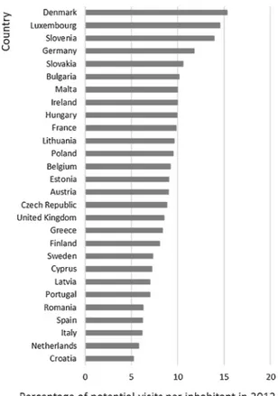
Highly populated countries, such as Germany, France and the United Kingdom, have larger actual flow because of the high demand for nature-based recreation driving the actual flow of the service. For a more meaningful comparison of the actual flow across countries, the use of the service needs to be expressed in relative terms, as the per-centage of potential visits per inhabitant.Fig. 7shows that Denmark and Luxembourg have the highest percentage of potential visits per inhabitant. This can be explained by the low proportion of the popu-lation considered as ‘unmet demand’ (22% in Denmark and 10% in Luxembourg), but also by a higher share of the population living very close (less than 2 km) to ‘high-quality areas for daily recreation’. Within this distance, the percentage of citizens engaging in ‘daily nature-based recreation’ is higher than further away (Fig. 4).
3.4. Accounting tables
At the EU level, the actual flow of nature-based recreation was va-lued at approximately EUR 50 billion in 2012. The supply table for nature-based recreation shows that woodland and forest are the eco-systems with the highest value at the EU level (Table 3). However, the country-level accounting Tables (Appendix E) show that different countries record higher nature-based recreation for different ecosystem types. For example, in the United Kingdom a high actual flow is
recorded for grassland, while in other countries, such as Germany, Italy and Poland, woodland and forest provide the highest actual flow.
Table 3reports the data in absolute terms. However, the actual flow expressed in relative terms as the value of potential visits per inhabitant shows a remarkable change in the ranking of countries (Fig. 8).
Germany is the most populated country in Europe and it records the highest value for nature-based recreation in absolute terms. If we consider the value of recreation per total inhabitants, then Estonia, Hungary and Slovakia record the highest values, while Germany ranks ninth.
3.5. Benefit assessment
We found a non-significant correlation between the actual flow of daily nature-based recreation in 2012 and the proportion of the popu-lation with different levels of satisfaction with recreational and green areas (Table 4). However, the proportion of the population considered as ‘met demand’ has a significantly positive correlation with the pro-portion of people highly satisfied with recreational and green areas. This demonstrates that countries with higher recreation potential within 4 km of residential areas, as assessed in this study, have greater satisfaction with recreational and green areas as measured by the sta-tistical indicator relevant to personal wellbeing. Measurements to re-duce the unmet demand (population living beyond 4 km from recrea-tional areas) may significantly contribute to increasing the level of satisfaction with recreational and green areas.
3.6. Trends in nature-based recreation
The actual flow of nature-based recreation increased by about 26% between 2000 and 2012. A more detailed analysis of the drivers of change in the service flow shows that the overall increase in the use and value of the service is mainly due to the increase in the recreation potential of 23%. To a lesser extent, the increase in the demand (po-pulation) of about 6% also plays a role in driving changes in the actual flow of the service.
For all EU-15 countries, the increase in recreation potential was significantly larger than the increase in demand, improving their si-tuation to potentially satisfy the demand for recreation. Belgium and Ireland showed the largest increases in the actual flow of the service (Fig. 9). However, whereas in Belgium the main driver of change in service use was an expansion of recreational areas, in Ireland this was not as important. Instead, the increase in the actual flow was also driven by higher demand.
4. Discussion
Ecosystem services accounting is a very useful tool to assess the role of ecosystems and socio-economics systems determining the ecosystem services flow, and to measure changes arising from the interaction of different ecosystem service components – service potential and demand (Fig. 1). The experimental accounts for nature-based recreation devel-oped in this study show the importance of spatially explicit models for assessing ecosystem services, in which different components can be mapped – ecosystem service potential, demand and actual flow in both biophysical and monetary units. Deriving maps of ecosystem service potential and demand is a key step in quantifying the actual flow of the service used, which is determined by the spatial relationship (i.e., proximity in the case of nature-based recreation) between SPA and SBA. In addition, spatially explicit data on the components of ecosystem services (i.e., maps) are useful for understanding the role of different drivers behind changes in the service flow and for supporting policy decisions related to the management of natural capital.
In this experimental account, we focused on assessing only daily nature-based recreation, without accounting for visits to natural areas for which motor transport is required. Therefore, what we present is
only one of a range of nature-based recreation possibilities and the results should be interpreted in the context of what is being measured. Different results would have been obtained if the focus was on areas that were far away from roads and settlements or those with medium potential for nature-based recreation. For this last option, a new method should have been developed, able to attribute different value to the different nature-based alternatives (i.e., areas far away and/or with medium recreation potential).
4.1. Ecological models in ecosystem services accounts
This study presents one of the first approaches of ecosystem services accounting at the EU level, following the guidelines provided in SEEA EEA and the SEEA technical recommendations (UN, 2017; UN et al., 2014b). National accounts are usually based on official data/statistics reported by countries; however, as illustrated in this study, accounts for ecosystem services require the use of spatially explicit models of eco-system services. Models were needed because data on the number of users related to daily nature-based recreation activity were missing. These data could be used to quantify the actual flow and the economic value of nature-based recreation. Some Member States (e.g., Italy and the United Kingdom) have started to collect nature-based recreation data (ISTAT, 2018; UK Government, 2014). However, using data on the real use of nature-based recreation would lack a linkage with ecosystem service potential, failing to capture the role of drivers of change in ecosystem service flow, namely service potential and demand (Fig. 9). In other words, we might find an increase in the number of users of green areas simply because the population has increased. The increase in actual flow driven by growth in demand could be masking changes in recreation potential, such as a reduction in the extent or quality of
Table 3
Supply and use tables for daily nature-based recreation.
Type of economic unit Type of ecosystem unit Primary
sector Secondarysector Tertiarysector Households Rest ofthe world – exports
Green urban areas
Cropland Grassland Heathland
and shrub Woodlandand forest Sparselyvegetated land Wetlands Rivers and lakes Coastal and intertidal areas Nature-based recreation
EU-28, EUR million
Supply table 2000 83 3464 6221 2618 26,936 1148 2019 277 63 2012 83 4022 7499 3249 30,781 1546 2831 303 78 Use table 2000 42,829 2012 50,393
Fig. 8. Comparison between absolute and relative values of the actual flow for nature-based recreation in monetary terms (2012). Table 4
Correlation between the actual flow and the proportion of the population with their need for daily nature-based recreation covered (‘met demand’) with the proportion of the population showing different levels of satisfaction with green and recreational areas.
Proportion of population with different levels of satisfaction with recreational and green areas (2012)
High Medium Low
Actual flow 0.00n.s. 0.08n.s. −0.04n.s. Proportion ‘met
demand’ 0.60** −0.22
n.s. −0.47*
Significance level: n.s., non-significant; **, < 0.01; *, < 0.05.
nature areas for recreation. In this sense, natural capital accounting would fail in its goal to measure changes in the stock of natural capital, as also formulated by Hein et al. (2016). Ultimately, data on the number of users would be useful to validate the model and relate real-use data to the ecosystem potential we modelled in this study.
Integrating spatial models in accounting is a key step in the devel-opment of robust accounts of ecosystem services, in which the spatial connection between ES potential and demand plays a key role. Ecosystem services integrate ecology and socio-economical analysis. In ecology, service potential is more frequently assessed than service de-mand, and the actual flow is only rarely quantified (Boerema et al., 2017; Mouchet et al., 2017; Verhagen et al., 2017). The assessment of the actual flow, required in accounting, involves a higher level of complexity that arises from integrating ecosystems (the service poten-tial) and socio-economic systems (the demand for the service). This integration, as demonstrated for nature-based recreation, requires the assessment of the spatial relationship between SPAs and SBAs. In the case of nature-based recreation, proximity between high-quality areas for recreation and population (users) is the key spatial parameter for estimating service flow using the mobility function. The spatial re-lationship between service potential and demand needs to be carefully established when quantifying the actual flow of ecosystem services; however, this relationship differs depending on the type of the eco-system service being assessed (Syrbe and Walz, 2012).
4.2. Flow of nature-based recreation: from ecosystems to people
Nature-based recreation accounts for 2012 show an actual flow of 40 million potential visits to ‘high-quality areas for daily recreation’, with a total value of EUR 50 billion. This demonstrates the important contribution ecosystems make to satisfy people's recreation needs, which has increased by 26% since 2000. Woodland and forest are the ecosystem types with the greatest contribution to the use of nature-based recreation by households, as shown in the supply and use tables. Households are the only economic agent considered a direct user of this service. Services related to tourism are a consequence of a high influx of visits to some natural area of interest: ad hoc satellite accounts are dedicated to tourism already (United Nations et al., 2010). The role of natural attractions in tourism should be further developed within these tourism satellite accounts for consistency with the core SNA and to avoid double counting.
The 40 million potential visits estimated in this study may look relatively small when compared with the approximately 500 million EU citizens. This is explained by three factors (in order of importance). First, the assessment of actual flow is based only on the proportion of the population considered as ‘met demand’ (i.e., living within 4 km of ‘high-quality areas for daily recreation’), which in the EU is 62% of the total population (Fig. 6). Second, the actual flow is calculated by a calibrated mobility function using an average percentage of visits of 17%. It implies that only this percentage of the ‘met demand’ visits ‘high-quality areas for daily recreation’ (Fig. 4). Third, the nature-based recreation potential includes only high-quality areas with high nature-based recreation opportunities that are close to settlements and roads. Therefore, the results should be interpreted given these assumptions. Loosening these rigid conditions would evidently increase the actual use reported in this paper.
In spite of the relatively small number of visits, the monetary value of nature-based recreation, estimated at EUR 50 billion annually, is higher than that of other ecosystem services at the European level. For instance, water purification is valued at EUR 16 billion per year (La Notte et al., 2017), while the value of total crop pollination in Europe amounts to EUR 14 billion per year (Gallai et al., 2009). Although there might be limits to comparing ecosystem services values based on dif-ferent valuation techniques, the threefold value of natubased re-creation may suggest a high importance of this service for society.
In fact, there is a growing demand for nature-based recreation in society, as shown by the positive population trends in the EU (except in Germany; Fig. 9). The increase in demand, but especially the en-hancement in recreation potential, led to an increase of 26% in the potential number of visits between 2000 and 2012 (Fig. 9), corre-sponding to an increase of 16% in the value of the service (Table 3). The increase in recreation potential is mainly due to two key drivers of the model: land cover and protected areas. In relation to land cover changes, ecosystem extent accounts, complementary to the service counts (SEEA EEA), would provide the data necessary to make an ac-curate interpretation of the role of land cover changes on increasing ecosystem service potential in each country. The key land-cover vari-ables leading to an increase in service potential are the expansion of forest and semi-natural areas. In some cases, urban sprawl may also play a key role if recreation hot spots become closer to residential areas, changing the spatial distribution between ecosystem services potential and demand.
Protected areas (‘Natura 2000’ sites), as included in the model, do not necessarily imply any improvement in the physical suitability or condition of the ecosystems supporting recreation. However, new pro-tected areas usually involve the development of recreation services and facilities, such as adding walking paths and informative signs about designated areas with high natural value, increasing the recreation potential. Although the nature-based recreation model excludes ‘strict nature reserves’ from analysis (where access is not permitted) (category Ia,Appendix C), recreational use of protected areas may compromise the conservation management of those areas. Ultimately, potential conflicts between nature conservation and recreation should be con-sidered in management strategies.
Working at the EU level imposes many limitations, such as data availability and consistency. As mentioned in Section2.3, for the bio-physical mapping, a procedure simplified from the original approach was applied, excluding data that cannot be compared over time such as High Nature Value Farmland (Paracchini et al., 2014). This may result in an underestimation of the ecosystem-based potential in some agri-cultural areas that should be taken into account. Availability of these data for different time periods would improve the assessment of changes in natural capital and the ecosystem services it provides. In addition, the mobility function for the EU-28 has been built using only data from England. The lack of data also prevented us from applying more appropriate valuation techniques, such as hedonic pricing, since spatially explicit data on housing pricing are not available at the EU level (European Environment Agency, 2010). Therefore, the travel cost method was the most suitable technique to calculate a proxy of the value of walking/biking trips consistently with the SNA. In future de-velopments of nature-based recreation accounts, alternative valuation methods, such as hedonic pricing, could also be compared once datasets become available. However, attention should be paid to harmonising this technique with SNA by avoiding double counting.
Another limitation of the valuation technique used is the lack of integration with congestion effects. Congestion is a social sustainability component that ideally would need to be accounted for when valuing the service in future applications. Crowded recreation areas may con-tribute less to wellbeing, thereby decreasing the benefit generated by the service and, consequently, its value. Congestion can also influence people to choose to go elsewhere if the location is too crowded, what is known as displacement (Manning and Valliere, 2001). One possible way of calculating congestion is to assess the number of visits per square metre of ‘high-quality areas for daily recreation’: the area's size on its own cannot provide a measurement for congestion unless it is considered together with the visiting ratio of the population. Where there are many inhabitants, larger-sized areas or many smaller-sized areas would be required to meet the demand for daily recreation in a socially sustainable way.
4.3. Application to land planning
The spatial analysis required for nature-based recreation accounting can be used to support policy decisions on land planning, to identify priority areas for ecosystem restoration. Priority should be given to enhancing the recreation potential of those areas with a high ‘unmet demand’ for the deployment of green infrastructure. This kind of measure can increase the equitability of access to natubased re-creation areas, and contribute to the achievement of the Sustainable Development Goal 11 (United Nations, 2015). As shown inFig. 6, 38% of the EU population has limited access to ‘high-quality areas for daily recreation’ (‘unmet demand’). Improving proximity to those areas (i.e., increasing the ‘met demand’) will have a positive impact on the po-pulation by increasing their level of satisfaction with recreational and green areas (Table 4), which is a component of life satisfaction. It is interesting to highlight that satisfaction with green areas is correlated with the proportion of the population with ‘met demand’, but not with the actual flow. This may suggest that those living within 4 km of ‘high-quality areas for daily recreation’ are also satisfied with the availability of recreational areas, regardless of the distance. This analysis con-stitutes an initial approach to assessing the benefits generated by nature-based recreation; however, further research would be needed to properly account for the benefits generated by visits to recreational areas. Importantly, the comparison of the nature-based recreation as-sessment with external and independent indicators, such as GREENSAT, may be interpreted as an ex-post validation of the assumptions made in our assessment, such as those taken for the delineation of ‘high-quality areas for daily recreation’ from the ESTIMAP model or the distances considered to distinguish between ‘met’ and ‘unmet demand’. 5. Conclusions
Ecosystem services accounting is still experimental and requires the development of a number of accounts for different types of ecosystem services. Practical examples of ecosystem services accounts, as shown in this study, are required to further develop the conceptual and
methodological framework proposed by the SEEA EEA. This study, using nature-based recreation as an example, highlights the importance of spatially explicit models for ecosystem services accounts, in which the different components of ecosystem services can be mapped, i.e., potential, demand and flow. Spatial models of ecosystems services are also required to properly address the drivers of changes in ecosystem services: changes in ecosystems (extent and condition) and changes in socio-economic systems or the spatial relationship between ecosystems and socio-economic systems. In addition, using biophysical spatial models in ecosystem services accounts contributes to the development of policy measures targeting the enhancement of natural capital, eco-system services and the benefits they provide.
The accounting tables completed for a representative number of ecosystem services may become a useful tool to aid the analysis of sy-nergies and trade-offs among services, including provisioning, regula-tion and maintenance, and cultural ecosystem services. Consistently applying the same accounting methodology across EU Member States will enable accurate comparisons between countries and over time. This is undertaken by employing the mechanism and rules of the SNA and the SEEA-EEA, allowing the integration of ecosystem services with traditional economic accounts so that environmental-economic ana-lyses can be undertaken.
Acknowledgments
The content of this publication does not reflect the official opinion of the European Union. Responsibility for the information given and views expressed in this paper lies entirely with the authors. This paper is a contribution to the phase 2 Knowledge and Innovation Project on an Integrated System of Natural Capital and Ecosystem Services Accounting in the EU (KIP INCA). This paper greatly benefited from the advice and comments of the KIP INCA partners and other colleagues on an earlier version: ESTAT (Anton Steurer, Lisa Waselikowski, Veronika Vysna); DG ENV (Laure Ledoux, Jakub Wejchert); EEA (Jan-Erik Petersen, Markus Erhard); and RTD (Nerea Aizpurua).
Appendix A. List of input data for the biophysical assessment of nature-based recreation. Ecosystem service component Variable Temporal
cov-erage Data source Ecosystem service
potential EB-P Land use (CORINE Land Cover) 2000, 2006,2012 CORINE Land Cover from the European Environment Agency(http://www.eea.europa.eu/data-and-maps) Protected areas 2000, 2006,
2012 World Database on Protected Areas( https://www.iucn.org/theme/protected-areas/our-work/world-database-protected-areas)
Bathing water quality 2000, 2006,
2012 State of bathing water( https://www.eea.europa.eu/themes/water/status-and-monitoring/state-of-bathing-water/state/state-of-bathing-water-3)
Distance to coast (sea and inland
water bodies) 2000, 2006,2012 CORINE Land Cover 1990, 2000, 2006 and 2012 from the European Environment Agency(http://www.eea.europa.eu/data-and-maps) Coastal geomorphology 2000, 2010 EUROSION Coastal Erosion Layer (Eurosion 2005)
Human
in-puts Tele atlasResidential areas 20132000, 2006, “Tele Atlas Map Insight”. Tele Atlas. Retrieved 2013 2012 CORINE Land Cover from the European Environment Agency(http://www.eea.europa.eu/data-and-maps) Demand Local administrative units (LAUs) 2015 http://ec.europa.eu/eurostat/web/nuts/local-administrative-units
Population 2000, 2015 Global Human Settlement Layer (http://ghsl.jrc.ec.europa.eu/ghs_pop.php)
Appendix B. Suitability of land to support nature-based recreation based on expert-based scoring
Grid code Corine land cover Score
1 Continuous urban fabric 0
2 Discontinuous urban fabric 0.1
3 Industrial or commercial units 0
4 Road and rail networks and associated land 0
5 Port areas 0
6 Airports 0
7 Mineral extraction sites 0
8 Dump sites 0
9 Construction sites 0
10 Green urban areas 1
11 Sport and leisure facilities 0.1
12 Non-irrigated arable land 0.3
13 Permanently irrigated land 0.3
14 Rice fields 0.4
15 Vineyards 0.5
16 Fruit trees and berry plantations 0.5
17 Olive groves 0.5
18 Pastures 0.6
19 Annual crops associated with permanent crops 0.3
20 Complex cultivation patterns 0.3
21 Land principally occupied by agriculture, with significant areas of natural vegetation 0.6
22 Agro-forestry areas 0.6
23 Broad-leaved forest 1
24 Coniferous forest 0.8
25 Mixed forest 1
26 Natural grasslands 0.8
27 Moors and heathland 0.8
28 Sclerophyllous vegetation 0.8
29 Transitional woodland-shrub 0.8
30 Beaches, dunes, sands 1
31 Bare rocks 0.8
32 Sparsely vegetated areas 0.7
33 Burnt areas 0
34 Glaciers and perpetual snow 0.8
35 Inland marshes 1 36 Peat bogs 0.8 37 Salt marshes 1 38 Salines 0.8 39 Intertidal flats 1 40 Water courses 1 41 Water bodies 1 42 Coastal lagoons 1 43 Estuaries 0.8
44 Sea and ocean 1
Appendix C. Cross-tabulation between management objectives and IUCN categories with the related scores for the recreation potential map
Management objective IUCN category
Ia Ib II III IV V VI
Protection of specific natural/cultural features – – 2 1 3 1 3
Tourism and recreation – 2 1 1 3 1 3
Education – – 2 2 2 2 3
Sustainable use of resources from natural ecosystems – 3 3 – 2 2 1
Maintenance of cultural/traditional attributes – – – – – 1 2
Score for the recreation potential map 0.0 0.6 0.8 0.6 0.6 1.0 0.8
Key: 1 primary objective; 2 secondary objective; 3 potentially applicable objective; − not applicable. Derived and modified fromEagles et al. (2002).
Appendix D. Illustration of the distance buffers from ‘high-quality areas for daily recreation’ in the surroundings of an urban area (Padova, Italy)
In red appear populated areas. In these areas, the number of inhabitants is then summed up for the different distance buffers where they are located. Green-shade scale buffers correspond to areas where the proportion of the population whose need for daily nature-based recreation is covered (‘met demand’). Grey areas represent the locations where the population without guaranteed access to ‘high-quality areas for daily re-creation’ (‘unmet demand’).
Appendix E. Extended supply and use tables for EU Member States Table E1 Supply table for year 2000.
Type of economic unit Type of ecosystem unit
Primary
sector Secondarysector Tertiarysector Households Rest ofthe world – exports
Green urban areas
Cropland Grassland Heathland
and shrub Woodlandand forest Sparselyvegetated land
Wetlands Rivers
and lakes Coastaland inter-tidal areas
Nature-based recreation
EUR million, year 2000
AT 0.74 24.22 67.86 25.72 333.34 76.96 5.75 4.64 – BE 2.65 71.15 64.91 23.30 401.22 2.70 17.90 4.60 3.10 BG 0.19 5.55 23.87 10.01 177.08 10.06 1.73 2.58 0.14 CY 0.22 0.44 0.22 3.71 34.43 1.10 0.12 0.45 0.38 CZ 0.48 78.16 60.40 0.84 489.06 0.14 4.30 1.76 – DE 37.08 1024.8 1956.62 87.11 8949.42 31.97 124.77 110.52 25.51 DK 12.21 126.12 92.67 106.75 459.38 17.73 135.17 6.05 44.71 EE 0.29 2.00 8.56 1.44 83.44 1.08 37.91 2.48 0.47 EL 0.07 75.87 128.68 211.90 549.10 39.71 9.79 6.32 13.81 ES 0.68 230.90 268.43 499.24 1221.61 93.88 14.81 16.56 21.23 FI 0.02 1.31 2.43 86.86 432.82 20.71 126.08 11.70 0.69 FR 1.36 367.80 706.41 130.42 2270.17 180.88 36.81 46.83 31.14 HR 0.30 11.52 19.03 5.85 152.70 3.00 7.72 6.79 0.24 HU 0.87 50.02 195.41 – 657.06 2.27 64.73 32.26 – IE 0.08 3.46 12.93 8.08 13.88 9.76 87.55 3.06 2.50 IT 2.51 259.63 420.53 257.45 2518.40 285.50 13.11 21.80 11.99 LT 0.30 20.04 5.50 0.43 111.60 0.35 7.65 3.21 0.01 LU 0.09 3.73 3.56 – 92.03 – – 0.34 – LV 0.25 11.38 6.90 – 86.80 0.21 10.31 1.81 0.01 MT 0.26 2.25 – 3.82 0.34 0.49 – – 0.16 NL 6.00 19.55 197.74 104.10 537.72 32.70 129.84 825.23 24.73 PL 1.50 382.53 355.95 1.92 3503.96 5.83 57.42 49.71 0.02 PT 0.27 254.93 52.07 199.39 744.65 40.61 1.50 10.96 41.87 RO 0.20 9.86 32.35 8.16 204.08 4.31 90.67 13.88 1.49 SE 0.97 2.94 21.58 241.32 611.41 83.31 134.65 33.02 0.34 SI 0.12 7.79 3.29 6.70 69.08 8.89 0.21 0.83 0.39 SK 0.15 56.47 58.38 9.13 851.81 7.63 2.79 4.89 – UK 7.84 318.97 1257.08 486.54 715.71 152.10 777.52 7.19 42.71 EU 77.68 3423.4 6023.36 2520.19 26,272.29 1113.9 1900.83 1229.49 267.63
Table E2 Use table for year 2000.
Type of economic unit Type of ecosystem unit
Primary
sector Secondarysector Tertiarysector Households Rest ofthe world – exports
Green urban areas
Cropland Grassland Heathland
and shrub Woodlandand forest Sparselyvegetated land Wetlands Rivers and lakes Coastal and inter-tidal areas Nature-based recreation
EUR million, year 2000
AT 539.22 BE 591.51 BG 231.21 CY 41.07 CZ 635.13 DE 12,347.81 DK 1000.79 EE 137.67 EL 1035.25 ES 2367.35 FI 682.62 FR 3771.81 HR 207.15 HU 1002.62 IE 141.30 IT 3790.91 LT 149.10 LU 99.75 LV 117.67 MT 7.32 NL 1877.60 PL 4358.84 PT 1346.25 RO 365.01 SE 1129.54 SI 97.30 SK 991.25 UK 3765.67 EU 42,828.74
Table E3 Supply table for year 2012.
Type of economic unit Type of ecosystem unit
Primary
sector Secondarysector Tertiarysector Households Rest ofthe world – exports
Green urban areas
Cropland Grassland Heathland
and shrub Woodlandand forest Sparselyvegetated land
Wetlands Rivers
and lakes Coastaland inter-tidal areas
Nature-based recreation
EUR million, year 2012
AT 1.01 34.69 93.19 33.19 456.08 95.32 7.44 6.55 – BE 2.57 89.36 90.81 15.40 678.66 1.76 12.35 4.61 5.51 BG 0.20 85.76 100.39 7.06 791.43 12.49 2.69 13.94 0.17 CY 0.18 2.08 1.56 13.50 40.99 2.20 0.10 0.60 0.37 CZ 0.43 72.10 78.59 0.68 564.42 0.12 4.55 3.43 – DE 28.94 876.96 1782.37 68.42 7732.75 21.45 103.47 96.47 20.12 DK 11.38 123.72 75.37 84.51 406.02 14.19 104.11 8.04 39.54 EE 0.43 10.27 8.90 1.25 154.75 0.56 39.15 1.49 0.17 EL 0.08 74.61 92.03 148.40 362.03 25.67 5.37 4.87 7.08 ES 1.16 373.79 433.70 762.67 1864.78 136.36 21.45 29.14 30.21 FI 0.02 2.14 1.96 70.33 394.19 16.78 103.50 11.80 0.60 FR 2.18 546.22 1060.64 212.32 3568.07 228.13 45.53 66.57 37.19 HR 0.25 12.36 16.88 5.73 145.83 2.65 6.40 5.83 0.27 HU 1.04 99.56 358.07 – 1345.29 2.59 85.05 64.86 – IE 0.15 11.27 34.95 14.71 52.39 16.20 169.06 5.57 4.75 IT 4.25 387.19 569.86 350.20 3463.47 405.56 18.15 34.50 15.34 LT 0.59 42.27 13.71 0.77 282.63 0.67 15.40 7.03 0.02 LU 0.05 4.68 3.16 – 54.34 – 0.01 0.17 – LV 0.25 10.64 7.72 – 83.12 0.49 9.95 1.85 0.01 MT 0.40 5.51 – 8.00 0.56 0.73 – – 0.32 NL 4.80 19.02 134.90 64.95 346.16 19.97 86.13 480.76 14.64 PL 1.29 311.70 346.51 1.34 2836.67 4.21 41.62 45.26 0.10 PT 0.31 278.49 52.06 202.85 799.43 41.59 1.56 15.85 44.36 RO 0.34 71.34 234.43 22.81 1208.06 6.72 115.91 45.47 1.69
SE 1.07 3.87 20.27 220.73 676.11 75.84 134.49 38.28 0.35
SI 0.05 15.41 11.36 3.04 159.04 3.76 0.73 1.01 0.14
SK 0.18 73.96 73.97 7.63 1210.04 6.60 3.08 6.86 –
UK 13.47 434.07 1784.59 776.16 1045.78 208.75 1158.70 14.18 55.86
EU 77.08 4073.05 7481.97 3096.66 30,723.08 1351.3 2295.95 1014.96 278.82
Table E4 Use table for year 2012.
Type of economic unit Type of ecosystem unit
Primary
sector Secondarysector Tertiarysector Households Rest ofthe world – exports
Green urban areas
Cropland Grassland Heathland
and shrub Woodlandand forest Sparselyvegetated land Wetlands Rivers and lakes Coastal and inter-tidal areas Nature-based recreation
EUR million, year 2012
AT 727.48 BE 901.03 BG 1014.13 CY 61.58 CZ 724.33 DE 10,730.96 DK 866.89 EE 216.95 EL 720.15 ES 3653.25 FI 601.33 FR 5766.85 HR 196.21 HU 1956.46 IE 309.04 IT 5248.52 LT 363.10 LU 62.41 LV 114.03 MT 15.51 NL 1171.32 PL 3588.69 PT 1436.49 RO 1706.77 SE 1171.02 SI 194.53 SK 1382.32 UK 5491.55 EU 50,392.90 References
Bagstad, K.J., Villa, F., Batker, D., Harrison-Cox, J., Voigt, B., Johnson, G.W., 2014. From theoretical to actual ecosystem services: mapping beneficiaries and spatial flows in ecosystem service assessments. Ecol. Soc. 19, 64. https://doi.org/10.5751/ES-06523-190264.
Barton, H., Tsourou, C., 2013. Healthy Urban Planning. Routledge, London.
Boerema, A., Rebelo, A.J., Bodi, M.B., Esler, K.J., Meire, P., 2017. Are ecosystem services adequately quantified? J. Appl. Ecol. 54, 358–370. https://doi.org/10.1111/1365-2664.12696.
Bowler, D.E., Buyung-Ali, L.M., Knight, T.M., Pullin, A.S., 2010. A systematic review of evidence for the added benefits to health of exposure to natural environments. BMC Public Health 10, 456.https://doi.org/10.1186/1471-2458-10-456.
Burkhard, B., Maes, J., 2017. Mapping Ecosystem Services. Pensoft Publishers, Sofia, Bulgaria.
Dudley, N. (Ed.), 2008. Guidelines for Applying Protected Area Management Categories. IUCN, Gland, Switzerland. Retrieved fromhttps://portals.iucn.org/library/sites/ library/files/documents/PAG-021.pdf.
Eagles, P., McCool, S., Haynes, C., 2002. Sustainable Tourism in Protected Areas: Guidelines for Planning and Management. IUCN, Gland, Switzerland/Cambridge, UK. Ekkel, E.D., de Vries, S., 2017. Nearby green space and human health: evaluating
ac-cessibility metrics. Landsc. Urban Plan. 157, 214–220.https://doi.org/10.1016/j. landurbplan.2016.06.008.
European Commission-Joint Research Centre, Columbia University, Center for International Earth Science Information Network – CIESIN, 2015. GHS Population Grid, Derived from GPW4, Multitemporal (1975, 1990, 2000, 2015). European Commission and Joint Research Centre (Jrc) [Dataset]. Retrieved fromhttp://data. europa.eu/89h/jrc-ghsl-ghs_pop_gpw4_globe_r2015a.
European Environment Agency, 2010. Land in Europe: Prices, Taxes and Use Patterns, EEA Technical Report No. 4/2010. Office for Official Publications of the European Union, Luxembourg. Retrieved from https://www.eea.europa.eu/publications/land-in-europe.
Ferrini, S., Schaafsma, M., Bateman, I., 2015. Ecosystem services assessment and benefit transfer. In: Johnston, R.J., Rolfe, J., Rosenberger, R., Brouwer, R. (Eds.), Benefit Transfer of Environmental and Resource Values. Springer, Dordrect.
Fisher, B., Turner, R.K., Morling, P., 2009. Defining and classifying ecosystem services for decision making. Ecol. Econ. 68, 643–653.https://doi.org/10.1016/j.ecolecon.2008. 09.014.
Gallai, N., Salles, J.-M., Settele, J., Vaissière, B.E., 2009. Economic valuation of the vul-nerability of world agriculture confronted with pollinator decline. Ecol. Econ. 68, 810–821.https://doi.org/10.1016/j.ecolecon.2008.06.014.
Geurs, K.T., Ritsema van Eck, J.R., 2001. Accessibility Measures: Review and Applications, RIVM Report 408505 006. . Retrieved fromhttp://www.rivm.nl/ dsresource?.objectid=171931c0-1023-4d50-8a3e-99f8ea126b74&type=org& disposition=inline.
Ghermandi, A., 2015. Benefits of coastal recreation in Europe: identifying trade-offs and priority regions for sustainable management. J. Environ. Manage. 152, 218–229.
https://doi.org/10.1016/j.jenvman.2015.01.047.
GRASS Development Team, 2017. Geographic Resources Analysis Support System (GRASS) Software, Version 7.2. Open Source Geospatial Foundation. https://grass. osgeo.org.
Hein, L., Bagstad, K., Edens, B., Obst, C., de Jong, R., Lesschen, J.P., 2016. Defining ecosystem assets for natural capital accounting. PLoS ONE 11, e0164460.https://doi. org/10.1371/journal.pone.0164460.
ISTAT, 2018. Attività Ricreative. Retrieved from https://www.istat.it/it/archivio/attivit %C3%A0 ± ricreative (accessed March 2018).