UNIVERSIT `
A POLITECNICA DELLE MARCHE
Facolt`
a di Economia G.Fu`
a
DIPARTIMENTO DI SCIENZE ECONOMICHE E SOCIALI (DISES) Ph.D. degree in Economics - XXXI cycle
Doctoral Thesis
A Multi-parallel BMA approach
for Generalized Linear Models in Gretl
Author:
Luca Pedini
Supervisor:
Abstract
The impossibility of recognizing the Data Generating Process leads to poten-tial uncertainties in model specification that are often ignored in common selection methodologies: the model averaging approach is a promising alternative which di-rectly deals with this issue by simply considering a quantity of interest across the model space, with the obvious advantage of avoiding possible miss-specifications or wrong conclusions induced by the choice of a single “best” model.
From a practical viewpoint, model averaging belongs to both the Frequentist and the Bayesian framework, but in the present dissertation, I will follow the second one due to its major flexibility and potentiality: in particular, a Bayesian Model Aver-aging (BMA) scheme based on Markov Chain Monte Carlo (MCMC) simulations, which jointly samples parameters and models, is proposed for Generalized Linear Models. The interest in Generalized Linear Models finds its motivation in Microe-conometrics where, for instance, binary choice models are in common use and where the application of such techniques is still an unexplored field.
A software implementation in Gretl, via a package of functions, is then provided, having care of addressing new computational challenges, mainly the parallelization of the process via MPI (Message Passing Interface): parallelization is somehow a typical routine in standard Monte Carlo experiments, where, due to the independence of the sampling procedure, the maximal benefit in terms of CPU time gain could be achieved; however the same is not so straightforward in MCMC experiments. I will show how a simple application of parallelization in MCMCs is still useful, both in terms of a better exploration of model and parameter space and in terms of time savings. Finally, the afore-mentioned Gretl package opens the possibility of an automated procedure ready for use for the common user too, with the implicit recommendation of “reading carefully the package leaflet”.
The economic implications of model averaging are explored in a Treatment Evalu-ation problem with Propensity Score matching: model averaging is commonly used in forecasting problems with linear models, where the driving-idea of producing an esti-mate which balances the ones of each specification (properly weighted) leads to more robustness with respect to “guessing” any single one. In Propensity Score evaluation the choice of which variables should be included is often ignored, and the consequent specification could be determinant in the final treatment effect estimation; a simi-lar argument can be, therefore, applied: could model averaging be profitable in the Propensity Score definition instead of guessing which variable should be included?
I will investigate, as empirical illustration, the economic effect of tax rebates on consumption, using as case study the 2014 Italian income tax rebate, which intro-duced an increase in individual monthly salary of 80e to employees. A dataset from
4
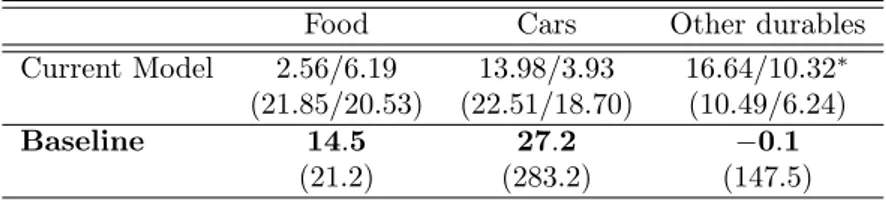
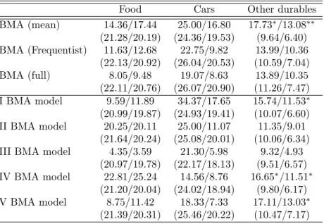
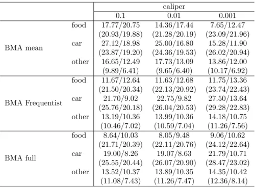
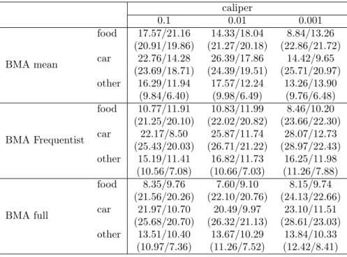
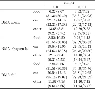
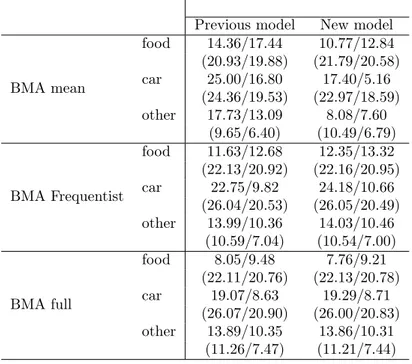
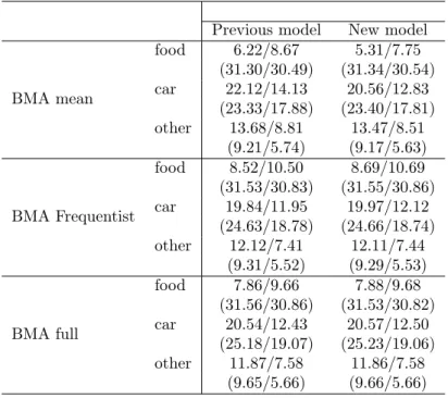
the “Survey on Household Income and Wealth” (SHIW) held by the Bank of Italy is built and three different techniques concerning model averaging are compared: a first one, which uses the model averaged posterior mean of the parameter of interest to build the Propensity Score, and then performs matching and treatment evaluation in the Frequentist manner; a second one averages the Frequentist treatment effects across the different models recognized by the BMA procedure, using as weight the posterior model distributions; and finally, a fully Bayesian procedure in which each sampled parameter by the BMA procedure defines a propensity score used to derive a model specific treatment effect, which is then aggregated according to the model probabilities. Matching is performed via pairwise nearest neighborhood under dif-ferent caliper and difdif-ferent data order: the last two BMA methodologies balance the estimates between different specifications, leading to a treatment evaluation less affected by the discretion in the choice of which variables include in the Propen-sity Score definition; the first proposed BMA technique, instead, does not always guarantee this condition. Moreover, it manifests a higher variability across different matching set-ups, as opposed to the fully Bayesian method which shows the highest robustness taking into account an additional source of uncertainty: the propensity score distribution.
Acknowledgments
I believe that words are imperfect means for perfect purposes, they can convey wonderful ideas, but in the end they are not complete since they are affected by interpretation, any word has a certain degree of vagueness.
However, words in their uncertainty, can express emotions: a good writer (not my case) would keep the reader stuck in his story; a good storyteller would charm people with his speeches; a good philosopher would make people wonder about what he has said.
The word is an art which, in its incompleteness, is a channel for that secret chamber inside each one, which hides different thoughts, different memories, different sensations: those aspects which are fragments of a whole puzzle, in which every individual has its own dimension.
For this reason, I would like to use, here, some words to thank those people who think have contributed to my life so far, and especially to these last three years (only three?!) of PhD.
I would start by thanking my family, for all the support provided so far, even though we have come across bad and good moments, I can always count on you, my dear family.
I would thank, then, my “big and little” brother Federico: despite the distance and the different routes we have decided to follow, it is like we are the same little boys we used to be.
My thanks also goes to all the people, friends, that I have met during my uni-versity studies and have decided to be by my side till now, thank you Silvano and Elisabetta.
I thank my colleagues, and in particular Andrea, Diego, Gloria, Raffaele, Sabrina, Thomas and Visar for every single discussion, fun moment that we had. Special mentions to Emanuele, Chiara and Francesco: I would like to thank Emanuele for the time we worked in the same “office” and for every single chat we had.
As regards Chiara and Francesco, probably this whole section would not be enough to express my sincere gratitude since their contribute is far beyond what common words can say: they have accompanied me in every step, they have “put up with” my craziness and together we have shared a lot of experiences. It is quite rare to find such good companions, and I sincerely hope that we will travel together for a little bit longer.
Last, but not the least, I would like to thank my supervisor and mentor Jack: if I had not attended his Econometrics class seven years ago, I would have had another job now, probably much more boring. Thanks to him, I have appreciated
6
the craftsmanship, which lies inside the world of Econometrics, and thanks to him I have known the Gretl project. He is truly an inspiration to me.
Thanks to you all, Luca
Contents
Abstract 3 Acknowledgments 5 1 Literature review 9 1.1 Introduction . . . 9 1.2 Selection . . . 101.2.1 Selection based on Information . . . 12
1.2.2 Selection based on Testing . . . 14
1.2.3 Model Confidence Set . . . 16
1.2.4 Shrinkage regression and LASSO type estimators . . . 17
1.3 Model Averaging . . . 19
1.3.1 Frequentist Model Averaging . . . 20
1.3.2 Bayesian Model Averaging . . . 26
1.3.3 BMA in practice . . . 36
2 RJMCMC and Parallelization in Gretl 39 2.1 Statistical background: GLMs . . . 40
2.2 BMA in GLMs: a brief overview . . . 43
2.3 Reversible Jump Markov Chain Monte Carlo . . . 44
2.3.1 An automated RJMCMC for GLM . . . 46
2.3.2 Prior choices and how to approximate µ and V . . . 47
2.3.3 The RJMCMC “in a nutshell” . . . 48
2.4 Parallel MCMCs . . . 49
2.4.1 Convergence in parallel . . . 51
2.5 The package . . . 54
2.5.1 The public function . . . 54
2.5.2 Private functions: the model ID set-up . . . 56
2.5.3 Private functions: the RJMCMC . . . 57
2.5.4 Private functions: the model dynamics . . . 57
2.5.5 MPI implementation . . . 58
2.5.6 A brief analysis of currently available RJMCMC and BMA packages . . . 60
2.6 Empirical example . . . 62
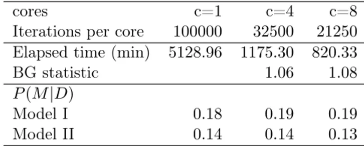
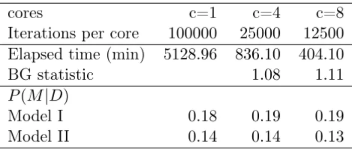
2.6.1 The importance of being parallelized . . . 66
2.6.2 Summary . . . 67 7
8 CONTENTS 3 A BMA analysis of Propensity Score Matching 69
3.1 Introduction . . . 69
3.2 Propensity Score matching and uncertainty . . . 71
3.2.1 A quick overview on Propensity Score . . . 71
3.2.2 The Bayesian Treatment evaluation . . . 72
3.2.3 Model Uncertainty issues . . . 74
3.3 Empirical analysis . . . 76
3.3.1 The 80e tax credit and some economic background . . . 77
3.3.2 Dataset and a first analysis . . . 79
3.3.3 A Bayesian Model Averaging counter-analysis . . . 83
3.3.4 More checks . . . 87 3.3.5 An additional experiment . . . 91 3.3.6 Summary . . . 93 Conclusion 95 Bibliography 97 Appendices 109 A Balancing properties 111
B RJMCMC output for the miss-specification example 115
C Parallelization in the tax rebate example 117
Chapter 1
Literature review
1.1
Introduction
Economists have inherited from physical sciences the myth that scientific inference is objective, and free of personal prejudice. This is utter nonsense. All human knowledge is human belief; more accurately human opinion. What often happens in physical sciences is that there is a high degree of conformity of opinion. When this occurs, the opinion held by most as asserted to be an objective fact, and those who doubt it are labeled as “nuts”. [...] The false idol of objectivity has done great damage to economic science.
E. Leamer, 1983
By using these words Edward Leamer cast doubt on most empirical works of the time: Economics was apparently following the right route, but in the end, it was just wandering into the fog: as is often the case, practitioners had in mind a representation of the reality, which, in theory, should have helped to simplify the understanding of the world, but in practice was advocated as an absolute truth.
This misleading behavior was mainly due to two different tendencies: a theory-driven one where empirical results were secondary and on the other hand, just the opposite, a data-driven approach. The former could easily lead to a dogmatic and aseptic scenario where theory is totally disconnected from reality; whereas the latter is what Leamer would address as Sherlock Holmes inference (Leamer, 1974, 1983), where the detective weaves together all pieces of the evidence into a plausible story, what is inferred without data is considered biased and finally the “culprit” confess! The consequence is the impoverishment of the Science, with even worst effects when this is translated into action.
It is quite clear how both approaches are not antithetical but should coexist and a fair compromise is the equilibrium between what can be inferred from data, what data really say and what the scientist has in his mind. Science is a public process, where ideas are continuously judged; nothing, in general, is eternal just because is human thought1: if exceptions are initially regarded with suspicion, when many
appear, a shift in knowledge (Kuhn, 1962; Lakatos, 1976) occurs which reshapes previous thoughts. The main ingredient and, at the same time, the main output of the whole process is the notion of model. A model is a simplification of the
1
Leamer (1974).
10 CHAPTER 1. LITERATURE REVIEW world, a caricature that cannot say the whole story in every detail, but can help in understanding the main drivers of a phenomenon thanks to its simplicity, in a similar fashion as a geographical map leads to a destination even though it does not represent the real space2.
This line of reasoning becomes particularly interesting in Economics, where there is no room for a correct experimental design like in physical sciences: the object of interest is the human behavior whose determinants are variable, numerous and inter-dependent. A model in Economics still has a raison d’être, but it should be handled much more carefully, because of its complex nature: we have just partial informa-tion and the Data Generating Process (DGP) is even more mysterious than in other cases. When we hear about the bad consequences of econometric models we should ask whether the motivation lies in this miscalculation: to quote Hendry (1980), for many years economists have been proud of the discovery of some philosopher’s stone, but history teaches that transmuting metal into gold is a taboo.
Starting from this premise the correct way of facing the problem is not surely the fear of acting, but it should be the fear of not acting properly: in order to let Economics gain a “general” and “resonated” consensus, we should consider our “experimental” design accurately, the context, the analytical tools, their motivations and assumptions as expressed by Angrist and Pischke (2010).
What I will present in this Chapter is a brief overview of the main techniques of model building, in particular: Section 1 is concerned with the model selection approach, where, given a set of rival specifications the interest is in finding the best one according to some criteria; in Section 2, I will consider a totally different view: model averaging. The idea behind is that choosing a single model implies many uncertainties (Chatfield, 1995), so it could be a reasonable alternative calculating our interest quantities over a set of specifications, weighted according to the probability of each model to be “true”.
A final remark is necessary: model selection will be mainly analyzed from a Frequentist perspective, whereas model averaging from a Frequentist and Bayesian one; this choice can be motivated by the fact that Bayesian selection is extremely close, in the methodologies used, to the model averaging one, so I will postpone any comments in that Section.
1.2
Selection
The model building process could be thought, in its simplest form, as a reply to three main questions:
• Which kind of relationship exists between the variables? • Which variables are important?
• How to make proper inference once answered the previous ones? Using mathematical notation, we can represent a model as:
y= f (X) + ε
2
1.2. SELECTION 11 where y is the dependent variable, X the matrix of independent variables, ε the error term, and f() a generic function, such as a linear one (linear model).
Our set of questions could be reformulated in: how to choose f, which elements of X are relevant and how we can use the whole expression to make, for example, forecast or further analysis.
Unfortunately, the first topic will remain mostly unexplored in this work, not because of its lack of importance, but because some route choices have to be made; hence we will assume the functional form f() as known and fixed for each speci-fication: sometimes, actually quite often, this is synonymous with nesting, which actually leads to the second question, variable selection.
In this case, two key notions seem to be parsimony and encompassing. Let us suppose to choose between a general and a restricted model, i.e. obtainable omitting variables from the general one, regardless of the choice we incur in the so-called bias-variance trade-off: the more variables we use, the less we are prone to omit relevant information but at the potential cost of less efficiency (bigger variance); conversely if we use few regressors we may face the opposite problem, biases3.
The concept of parsimony tries to balance the two; a useful analogy could be the Occam’s razor principle: focusing only on the relevant information and shaving every useless repetition.
Encompassing is the tool used to reach this equilibrium: it is said of a model to encompass another one if it coveys the same amount of information, with the implicit consequence that a small specification encompassing a bigger one is a more appropriate choice (parsimony); the problem is how to establish this condition and following both the literature and the common routines applied in practice, the two major guidelines are surely Information measures and testing.
What is implicitly assumed throughout the thesis is the adherence to the so-called M-closed framework: in the Bayesian literature (Bernardo and Smith, 1994), model comparison problems can be distinguished into three different categories, the M-closed, the M-complete and the M-open settings. The M-closed one assumes that the DGP is included in the model space, i.e. the set of models of interest, and it represents the predominant assumption in both model selection and model averaging works. However, the underlying idea is quite restrictive, since DGP can be too complex or totally unknown, so more general perspectives, i.e. the M-complete and the M-open settings, could be necessary. In particular, the M-complete framework assumes that the DGP is known, but is too complex to be implemented and so it is excluded from the model space. In this way every specification is seen as an approximation which tries to balance accuracy and simplicity. The M-open setting is even more extreme, as it postulates either the totally ignorance of the DGP or the knowledge of it, but the impossibility of obtaining any consistent approximation4.
Despite the fact that this distinction has been enlarged to embrace the Frequentist
3
This is actually much more complicated: as explained in De Luca et al. (2018), adding more variables does not always mean reducing the bias of the parameter of interest, since this is only valid when the general model coincides with the DGP. When restricted and general models are both underspecified, i.e. smaller that the real DGP, adding more variables does not mean necessarily improving the omitting variable bias. Conversely, bigger specifications do not always lead to less efficient estimates: in homoskedastic linear models, restricted regression coefficients will be more efficient than the general counterparts, but the condition is no more guaranteed outside this context.
4
12 CHAPTER 1. LITERATURE REVIEW perspective, the M-complete and M-open assumptions are extremely challenging, even though some recent works have started to be concerned with them (Hoeting et al., 1999; Clyde and Iversen, 2013; Lu and Su, 2015; Zhang et al., 2016; Ando and Li, 2017); as a consequence any discussion related to these settings will be avoided and the M-closed framework is assumed unless otherwise specified.
Moreover, the general set-up assumes less regressors than observations (despite the brief overview in subsection 1.2.4), so big data analysis is not of primarily concern, but will be of course covered in future developments.
1.2.1 Selection based on Information
The idea behind the Information-based approach starts with the so-called Kullback-Leibler (KL) information measure (Kullback and Kullback-Leibler, 1951): given an unknown density function f and an approximation g(|θ) which depends on some parameters θ, the KL measure is defined as5:
KL(f, g) = ∫︂
f(x)[log f (x) − log g(x|θ)]dx = Ef[log f (x)] − Ef[log g(x|θ)] (1.1)
Equation (1.1) represents the discrepancy between the theoretical distribution and its approximation: the impossibility of knowing f (hence its expected value Ef[log f (x)])
and the parameter θ, which needs to be estimated, prevents us to employ (1.1) di-rectly. This turns out to be a minor issue, because the element Ef[log f (x)]simplifies
when comparing different models based on the same distribution, as in the following example
KL(f, gi) − KL(f, gj) = Ef[log f (x)] − Ef[log gi(x|θ)] − Ef[log f (x)] + Ef[log gj(x|θ)]
= Ef[log gj(x|θ)] − Ef[log gi(x|θ)]
where gi and gj correspond to two different model specifications.
We should, thus, restrict the attention to Ef[log g(x|θ)]. In this case, we
can-not directly compute this quantity because the expectation operator depends on f. However we could overcome this obstacle, by simply moving to Ey[Ef(log g(x|θ))],
where y denotes the data.
It can be proved, following Akaike (1998), that the log-likelihood of the selected model g(x|θ) evaluated in its maximum ̂θM L, i.e. log p(y|̂θM L) = l(̂θM L) plus a
correction term asymptotically equal to the number of regressors k, is an unbiased estimator of this quantity:
Ey[Ef(log g(x|θ))] = l(̂θM L) − k
this leads ultimately to the celebrated Akaike’s Information Criterion:
AIC = −2l(̂θM L) + 2k (1.2)
Given a set of concurrent models, the AIC identifies the loss given by the KL divergence, so hypothetically the specification which minimizes it, is the most adher-ent to f(x). From Akaike’s discovery, several aspects of the Information approach
5Notice that f does not depend on parameters. According to the original framework: “parameters
1.2. SELECTION 13 were questioned: the implicit assumptions that among the set of models the correct one exists or the asymptotic nature of the results. The former was dealt by Takeuchi (1976) with the derivation of a possible generalization, often named nowadays as Takeuchi’s Information Criterion (TIC, in brief). The second issue, instead, was partly addressed by Sugiura (1978); Hurvich and Tsai (1989) who derived a cor-rected version of AIC (AICc) when the sample is “relatively” small in relation to the
regressor number6. Both of them were characterized by the adjustment of the
penal-ized term 2k, which conducts to a even more general representation of Information Criteria:
IC = −2l(̂θM L) + p(n, k) (1.3)
where p(n, k) represents a penalty function depending on the sample size n and the number of regressors k. However, only Akaike’s IC and the two aforementioned extensions (TIC, AICc), following Burnham and Anderson (2003), are Information
Criteria per se, since they directly derive from the “Information theory”; a wide and quite acknowledged category composed by the Bayesian IC (BIC, Schwarz (1978)) or the Hannan-Quinn IC (Hannan and Quinn, 1979), despite the fact that they can be obtained from (1.3), convey a different information. Consider as an example the BIC:
BIC = −2l(̂θM L) + k log n
In Burnham and Anderson (2003), the BIC is categorized as a dimension con-sistent Information Criterion, which implies a balance between the loss given by the KL measure and the number of regressors, assuming that the fewer variables we use the better our approximation is. In other words if we assume a set of different specifications, a model which is favorite by the AIC, could be easily outperformed by another one according to the BIC if the difference in the KL is small and has fewer variables.
From a historical point of view, moreover, the BIC arises in Bayesian Statistics as a crude approximation of the posterior model probability, once a non-informative prior is assumed. We will deepen these definitions later, for the moment it is enough to state that by posterior model probability P (Mi|y), where y identifies the data and
Mi a specific model in a model space M, we mean the probability of the selected
specification to be the true one, after our initial idea provided by the prior is updated through the data. In particular, following Raftery (1995):
P(Mi|y) ≈
exp (−12∆BICi)
∑︁M
j=1exp (−12∆BICj)
where ∆BICi = BICi− BIC∗, with BICi as the BIC of the i-th model (Mi) and
BIC∗ as the minimum BIC obtainable in the set M.
It is quite clear how, at least from this perspective, the Bayesian Information Criterion has little to do with the KL measure in its original formulation, but actually, an artificial relationship can be built thanks to the general formula (1.3).
6The thumb rule is n/k < 40 where n and k are respectively the number of observations and of
14 CHAPTER 1. LITERATURE REVIEW
1.2.2 Selection based on Testing
The second, and probably most known, approach for undertaking model selection is testing, i.e. verifying if a parameter is significantly different from zero through a simple t-test or F-test7.
Despite its simplicity, many drawbacks can be found. The main one, in order of importance, is inferential: as noted in many works such as Chatfield (1995); Magnus and Durbin (1999) when a specification is selected, the inference is conditioned on that one, a fact that is quite often ignored. It can be shown that the conditioning is likely to imply biases in the estimator (if the selected model is not “true” or at least it is not a good approximation of the DGP), hence all derived conclusions could be misleading.
Another theme that happens to be crucial is the reuse of the same data set: virtuous practice implies the division of the sample into three different sets, a training set for estimation, a validation and testing one for verifying the fit. When the same data are repeatedly exploited for the same scope such as iteratively testing some hypothesis, i.e. data mining, spurious relationships may appear. Using an example illustrated by White (2000), let us suppose to send to a large number of individuals a free copy of a stock market newsletter: the group, in particular, is split into two on the basis of the type of the news, on the one hand an upward prediction, on the other a downward one. The next week only the group who receives the correct prediction will have a new copy, and the sub-division is then repeated. After several months there can still be a rather large group who have received perfect predictions, and who might pay for such “good forecasts”, but in fact, this is merely a coincidence!
Actually, the data mining problem deserves a closer look: especially in recent years, a renewed interest in the theme has been brought into attention thanks to the so-called machine learning techniques. Following these procedures, it is possible to build algorithms which, given a big dataset, can recollect the “correct” pattern among variables (a model) adjusting iteratively their output to the desired level of goodness of fit. It could appear a bit confusing considering data mining positively given the previous argument, but “carving” information in the same dataset could not be so negative if some conditions are met, such as high dimensionality of the sample.
A similar thesis is shown in our context of testing by White (1990): for a given set of models and a battery of tests, the more the sample size grows (toward infinity) and the smaller test sizes are employed, the more likely tests will select the correct specification. Thus type I and type II errors fall asymptotically to zero, and only the true specification survives8.
Therefore, stepwise procedures, i.e. testing iteratively if a variable is significant or not, could make sense provided asymptotic theory could apply and some further reg-ularities are met: two common views are specific-to-general and general-to-specific.
Specific-to-general starts with an essential specification, quite often the null model with the only constant as regressor, and then adds a variable at each step: if the addition improves the fit according to a goodness measure or simply through
7As a matter of fact there are also alternatives such as the more general Wald test, or the other
Likelihood based tests, such as the LM or LR tests.
8It is worth noting, however, that the bias issue illustrated at the beginning of the section still
1.2. SELECTION 15 a comparison test (F or W ) between the initial model and the new one, then the new variable is retained and the procedure is repeated. General-to-specific works in the opposite direction: a wide model (GUM, Generalized Unrestricted Model) is simplified till every remaining variable is rejected to be discarded.
PC-GETS and Autometrics
General-to-specific has known a very interesting development towards automati-zation in recent years: in case of linear or Augmented Distributed Lag (ADL) models it is possible to build a stepwise procedure with some interesting features known as PC-GEtS9(Hendry and Krolzig, 1999).
The differences with respect to the standard procedure mainly lie in10: a) the
validation of some desirable property on the residuals of each model (congruence11),
which, if not verified, prevents the deletion of the variable until the condition is restored; b) the dynamics of the deletions.
The removal of a regressor is analyzed through a multi-path search: every irrel-evant variable defines a deletion path in which the stepwise regression is separately held together with the congruence analysis and where each initial model has the related insignificant regressor omitted by default. With k irrelevant variables, multi-path search produces k final models that could be different, in which case the final choice is driven by the minimum BIC.
Deletions are performed via simple t-test or F-test in case of blocks of variables; moreover, in order to enhance the whole procedure, two common extensions are: pre-search, which runs initial significance tests with particularly high size to remove highly insignificant variables; and post-search (Hendry and Krolzig, 2004) which, in turn, implies the repetition of the multi-path search or a simplified version when different final specifications are obtained before advocating the use of BIC.
Automated GEtS possesses some interesting and potential pros such as consis-tency in model selection if all assumptions are met (Campos et al., 2003) and a possible extension if there are more variables than observations (Doornik, 2009b), but several cons too, which can be split into computational ones and statistical ones. In the first category we find the useless repetitions of the same models during multi-path search and the continuous congruence testing. Both of them are, in fact, dealt in an evolution of GEtS, Autometrics (Doornik, 2009a). Autometrics is based on the same principle with the not negligible difference of implementing a tree structure search, where from the initial GUM several branches, corresponding to models with an insignificant variable less, are produced via testing until the whole model space is analyzed, having care of skipping or pruning already encountered specifications: if a deletion test is rejected and a model could not be furthermore simplified it is named as “terminal”. Only terminals are tested for congruence: if this condition is not met, the model is discarded and we backtrack to its first parent which respects the criterion. All these models are then collected and the procedure repeated until only relevant variables are held or the most simplified congruent model is achieved.
9
PC-Gets is actually the name of the package which implements this procedure in the software Ox.
10
See Granger and Hendry (2005) for further details.
11It is a said of a model to be congruent if its residual are homoskedastic (both conditionally and
16 CHAPTER 1. LITERATURE REVIEW The statistical drawbacks, excluding the common stepwise issues12, concern
pri-marily the so-called cost of inference and cost of search, which, respectively, identify the problem of detecting relevant variables and of retaining insignificant ones. As a matter of fact, when a variable of interest has a near-zero value coefficient, the stepwise procedure struggles to retain it (Castle et al., 2013), while in the case of cost of search, unless we imply a strict significant test size α, we will always have an expected number of adventitious variables equal to ̄k = αk where k is the number of irrelevant covariates.
Finally, another aspect should be considered, the lack of flexibility: despite Au-tometrics seems to work even in more general context than linear models, this op-portunity does not seem fully explored; moreover when the congruence conditions are not met, it is not really clear how to proceed: it is possible to lower the tolerance (the size of the tests) but the properties of the whole procedure are not guaranteed anymore. For these reasons some alternatives are worth of interest.
1.2.3 Model Confidence Set
A quite different approach to selection, even though it is often categorized as a selection one, is the model confidence set (MCS) by Hansen et al. (2011). A very elementary introduction could be the following: building a set of models that contains the best one with a certain probability according to some criteria, in a similar way like the usual confidence interval works for estimators.
As a matter of fact, MCS aims to construct a set of plausible models with similar explicative power, so in general its definition becomes highly dependent on the data availability: with less informative data it is likely to have a wide model set (sometimes correspondent to the whole model space), whereas in the opposite case a small one13.
The formal description starts with a set of concurrent models M0, whose
ele-ments are checked via an equivalence test δMfor their equal “goodness”. When δMis
rejected, the equivalence is not verified, so an elimination rule eMdeletes the bad
per-formance models; the procedure is repeated until the first acceptance14 occurs. The
individual specifications inside M0 are evaluated in terms of a loss function LMi
15,
where Mi identifies the i-th element of M0. The losses are then mutually compared
using d(Mi, Mj) = LMi− LMj which is the main ingredient for the equivalence test;
it is possible to state the null hypothesis as:
H0 : E(d(Mi, Mj)) = 0 ∀ i, j ∈M0
where E() identifies the expected value operator. The whole algorithm is summarized as follows:
1. Define the set M0 and calculate d(Mi, Mj) = LMi− LMj for each element; 12
The afore-mentioned biases and small sample problems.
13
This feature opens the possibility of model uncertainty (Chatfield, 1995) as we will see more accurately in the next section.
14
The authors underline the similarity of the MCS procedure with the trace-test for selecting the rank of matrix such as Anderson (1984); Johansen (1988). Notice, moreover, that the problem of sequential testing, in this case, is avoided because the procedure is halted when the null is accepted.
15As an example if y is the dependent variable and ̂y its forecast, the loss is any function of their
1.2. SELECTION 17 2. Test H0 as above, via the equivalence test δM with size α;
3. If the null hypothesis is accepted, stop the precedure and define M0 =M∗1−α
where M∗
1−αis the Model Confidence Set for 1−α; otherwise use the elimination
rule to reduce M0 and repeat from Step 2.
As for the elimination rule we can assume many different formulations, as long as models contributing the most to E(d(Mi, Mj)) i.e. the worst ones, are erased
firstly; what should be verified is the so-called coherency between equivalence test and elimination rule. The coherency condition guarantees that the probability of our final model set asymptotically tends to the selected confidence 1 − α and from a practical point of view, it assures to avoid anomalies which can emerge from absurd combinations of δM and eM.
Finally, in Hansen et al. (2011) we found a disclosure of some common examples of equivalence tests and elimination rules too: some interesting ones can be mutated from the common quadratic-form test or t-test, whereas another category, based on linear regression models, is based on a likelihood framework which links MCS to the Information Criteria.
Except for the quadratic-form equivalence test which has a χ2 distribution, the
other ones do not have a standard one, so bootstrap methods are required with a slight modification to the original framework16.
1.2.4 Shrinkage regression and LASSO type estimators
The availability of bigger and bigger datasets, which turns to be a major theme in recent years, poses new questions and challenges to variable selection problems, in particular how to handle situations of few significant variables among a huge amount of not significant ones (sparsity), where there are potentially more regressors than observations.
Under this second scenario traditional least squares methods become problematic; consider as an example a linear model y = Xβ +ε where y is the dependent variable, X a matrix of regressors and ε the error term; then the solution of the optimization problem
min (y − Xβ)T(y − Xβ)
is not unique anymore17.
But even assuming less variables than observations in a big dataset with many regressors makes common selection routines unfeasible: quite rarely coefficients are set to zero during the estimation process so testing is strongly required, but as we have seen, spurious relationships may be included and biases can heavily undermine each conclusion. Information Criteria are equally troublesome, since all models need to be investigated, leading to a computational complexity which grows exponentially in the number of regressors (with k variables, 2k models are available).
16
It should be noted how de facto the quadratic-form has little application in practice compared to the correspondent t-test version: this is mainly due to the estimation of the variance matrix which could become easily not feasible.
17In this subsection I will focus on linear models, but the same argument can be easily extended
18 CHAPTER 1. LITERATURE REVIEW A plausible solution could be imposing some regularization inside the estimation procedure, which, loosely speaking, corresponds to imposing a constraint on the coefficients in the optimization problem of least squares:
min (y − Xβ)T(y − Xβ) subject to f(β) ≤ t (1.4)
with f() as a constraint function and t a given threshold.
Equation (1.4) identifies the shrinkage regression framework, where depending on the choice of the constraint function, different estimators with different properties are obtained. A common choice in variable selection problem seems to be the l1
norm ∥∥1, which leads to the celebrated LASSO estimator by Tibshirani (1996):
min (y − Xβ)T(y − Xβ) subject to ∥β∥
1 ≤ t (1.5)
Notice that the peculiar shape of the constraint imposes sparsity in the coeffi-cients, so not only some parameters are shrunk exactly to zero, but also assuming the number of significant regressors always smaller than the number of observations, implies the uniqueness of LASSO estimator even if there are more regressors than observations. Finally the choice of the threshold t is fundamental as well because it determines the magnitude of the shrinking effect: some common methods used for choosing this value range from cross-validation to the minimization of goodness of fit measures.
It appears that LASSO is the solution to all variable selection problems, but there are many aspects that merit a closer look: hypothetically, we would like to have a procedure which classifies all zero coefficients with probability tending to one and whose asymptotic distribution for non-zero coefficients is the same as if only those significant variables are included18. If this is the case, the obtained estimator
is defined as oracle efficient, but LASSO does not guarantee this condition; in fact, zero coefficients may have a probability mass at zero, but this probability is not tending to one and the non-zero coefficient estimates have an asymptotic bias.
An oracle consistent estimator could be easily obtained from LASSO by adjusting the shrinkage induced in the constraint function: Zou (2006) shows that weighing coefficients inside the penalty function by the inverse of the absolute value of their OLS estimate, produces a LASSO estimator with the oracle property (the so-called adaptive LASSO).
Some final remarks seem to be necessary since oracle property and adaptive LASSO have limitations: oracle property induces a problem of efficiency in the final estimator, and even if an equivalent condition for finite sample can be established, when data are not (much) sparse, the robustness of the procedure is affected. For these reasons second generation LASSO estimators (often named as debiased or desparsified LASSO19) have been introduced: these kind of methods simply estimate
standard LASSO coefficients in a first step, and then correct for their bias in the second one; it could be proven that debiased estimators are more efficient, robust and finally are easily usable for inference too20.
18Hence obtainable using simple least squares. 19
Van de Geer et al. (2014).
20Remember that LASSO requires simulated methods for inference or post-model-selection ones
1.3. MODEL AVERAGING 19
1.3
Model Averaging
Model building, as we have seen so far, is often concerned with the selection of an optimal model in order to explain data at best: the main issue is that, in practice, we do not know exactly the Data Generating Process (DGP), so we cannot have the certainty to choose the correct specification (model uncertainty); and if we still want to select one, we are prone to make inference conditional on this selection, often incurring in biases and, sometimes, in even worst consequences21.
Possible solutions are the aforementioned Model Confidence Set approach or shrinkage methods but in the model selection literature, an appealing alternative, which takes into account both previous problems, is known as model averaging22.
The idea of model averaging is quite simple: considering the estimates across many specifications, instead of focusing only on a single one and building the related in-terest quantity (e.g. a simple estimator or a forecast) as an averaged measure over the model space, i.e. the set containing models.
In mathematical terms: f(β)AV = M ∑︂ i=1 f(βi)ωi (1.6) 0 ≤ ωi≤ 1 M ∑︂ i=1 ωi = 1
where β is the parameter of interest, f() a generic functional form, βi and ωi are
respectively the parameter and the weight attached to the i-th model, where we assume that our model space M contains M different specifications.
The advantages of considering more than one model allow precisely to not ignore information that sometimes (actually quite often) the selection of a unique model excludes and that can be useful.
For this reason model averaging in Economics has quickly enjoyed popularity in recent years: in economic growth literature, for example, model averaging techniques have led to a much more complete and balanced inference about the growth determi-nants, with particular reference to the role of geography, integration and institutions, which were only partially analyzed in previous works. Some example of such model averaging literature are Brock and Durlauf (2001); Fernandez et al. (2001b); Sala-i MartSala-in et al. (2004); ESala-icher and NewSala-iak (2013); LenkoskSala-i et al. (2014); Durlauf (2018).
Koop et al. (1997), instead, exploits the use of Bayesian Model Averaging in au-toregressive (fractional) integrated moving average (ARIMA and ARFIMA) models for evaluating the real GNP; Cogley and Sargent (2005) consider the use of model av-eraging for analyzing inflation; Strachan and Van Dijk (2013) explore Bayesian Model Averaging methods with dynamic stochastic general equilibrium (DSGE) models, whereas George et al. (2008); Koop (2017) propose application of model averaging
21
Chatfield (1995) is a wonderful reference point for understanding the pros of model uncertainty.
22As a matter of fact model averaging can be considered as a shrinkage method too, at least in
20 CHAPTER 1. LITERATURE REVIEW to Vector Autoregression Models (VAR) 23. In Microeconometric literature some
examples are Van den Broeck et al. (1994) which deals with uncertainty in produc-tion modeling via stochastic frontier models or Sickles (2005) which examines firm inefficiency through Bayesian Model Averaging.
What remains to be explained is how to deal with model averaging; in particular, two main perspectives are available: on the one hand, the Bayesian viewpoint and on the other the Frequentist one. The former focuses on the posterior distribution of the parameter, so our f(β) is a density or a probability distribution; the latter, instead, simply replaces f(β) with the (Frequentist) parameter estimator, let us say
̂
β. The weight ωi represents in both cases a measure of the probability of a model
to be the appropriate one; in the Bayesian case we will use the so-called posterior model distribution, whereas in the Frequentist one some “Information Criteria” based measure.
Finally it is worth mentioning how the so-called hybrid methods have reached great consensus recently too. By hybrid methods we generally mean model averaging techniques which combine aspects from the Frequentist and Bayesian perspective in order to achieve a grater flexibility: the major examples are Bayesian Average of Classical Estimates (BACE) by Sala-i Martin et al. (2004), Weighted-Averaged Least Squares (WALS) by Magnus and Durbin (1999); Magnus et al. (2010) and Bayesian Averaging of Maximum Likelihood Estimates (BAMLE) by Moral-Benito (2012).
I will analyze only the strictly Bayesian and the strictly Frequentist method-ologies throughout this work, postponing the analysis of hybrid methods for future developments: I will start from the Frequentist Model Averaging (FMA) framework, where the main issues are how to deal with weights24and how to make inference with
the new averaged quantities (multimodel inference, Burnham and Anderson (2003)). I will then cover the Bayesian framework, having care of analyzing the main ingredi-ents of the recipe even though some details will be left for the next Chapter, where a suitable scheme for Generalized Linear Model is provided25.
1.3.1 Frequentist Model Averaging
Despite the fact that some applications of model averaging in a Frequentist sense can be dated back to Box and Jenkins (1970), a correct and rigorous dissertation of this method should be considered as a reply to some (computational) difficulties of its Bayesian counterpart. Since throughout this work I will favor the Bayesian perspective, I will try to sketch a brief description of FMA before the analysis of Bayesian Model Averaging: in doing so I will lose the chance of drawing any useful parallelism but the benefit will be a major adherence to the structure of this work.
In the FMA framework we are interested in weighing a Frequentist estimator ̂β or some function of it across several specifications; just as an example consider the linear model:
23
This is only a short overview of some applications of model averaging in Economics. For a more detailed analysis see Steel (2018)
24
Remember that the quantity of interest is simply the estimate of the parameter, which can be obtained straightforwardly in Frequentist case.
25
More detailed overviews on specific model averaging techniques include Clyde and George (2004); Claeskens and Hjort (2008); Wang et al. (2009); Moral-Benito (2015); Magnus and De Luca (2016); Steel (2018).
1.3. MODEL AVERAGING 21
y= Xβ + ε
where y is a n×1 vector of response variable, X is the n×k matrix of explanatory variables and ε the usual disturbance term.
Using the same notation of the previous section the Frequentist correspondent to equation (1.6) is: ̂ βAV = M ∑︂ i=1 ωiβ̂OLS,i, M ∑︂ i=1 ωi= 1
where ̂βOLS,i is simply the OLS estimator of the correspondent model, where we
set ̂βi,j = 0 if the j-th regressor is absent from the model i.
The definition of the weight ωi becomes crucial, since all the properties of the
averaged estimator are a consequence of this choice: there is not an unique solution and the possibility to make proper inference becomes unclear due to the complexity involved in the calculation of standard errors or asymptotic distributions (Burnham and Anderson, 2003, 2004).
Some common choices are presented in the following subsubsections. FMA with IC weights
One of the first method implied to calculate weights was due to Buckland et al. (1997): in particular recalling the definition of Information Criteria given in (1.3) and assuming the same notations as before,
IC = −2l(̂θM L) + p(n, k)
after some rearrangements and by taking the exponential operator we obtain a measure of the “penalized” likelihood:
exp(−1
2IC) = L(̂θM L) exp(− 1
2p(n, k)) (1.7) where L is the likelihood of the model. Normalizing (1.7) over the whole model space allows us to treat it as a probability, but also as a weight of the i-th model:
ωi = exp(−1 2ICi) ∑︁M j=1exp(−12ICj) (1.8) where to a higher ωi corresponds a high probability of the model to be plausible.
For computational easiness Burnham and Anderson (2004) proposes a slightly different version26: ωi= exp(−1 2∆i) ∑︁M j=1exp(−12∆j) (1.9) with: ∆i = ICi− ICmin 26
22 CHAPTER 1. LITERATURE REVIEW where ICmin is the minimum of the M different IC values.
As for the choice of the Information Criterion, Akaike’s Information Criterion (AIC) and Bayesian Information Criterion (BIC), with the same difference in usage as the one previously sketched in subsection 1.2.1, are the main options.
It is worth noting that a quite different alternative is provided in Hjort and Claeskens (2003) with the Focussed Information Criterion (FIC): while in IC model averaging the weight calculation does not consider the scope of the averaging proce-dure, mainly because the commonly applied IC are built for only model comparison purposes, the FIC and its derived weights are meant to take into account the “use” of the model. In other words it can easily happen that the weights chosen to be optimal for inference, cannot be equally good for forecasting or analysis of variance: in order to fulfill this task the author introduce an objective function of the parameter of interest, which embodies this “scope”27, and define a related Information Criterion,
the FIC, as asymptotic approximation of the Mean Squared Error of this function. A curious fact that deserves more attention and could affect the effectiveness of this measure is the dimensionality: it turns out that the structure of the chosen function could lead to have a multidimensional FIC (vector) for each model; in these cases its interpretation could be quite challenging and a lot depends on the context of the analysis.
FMA with Mallow’s C based weight
Information Criteria weights derived from AIC or BIC provide a compromise between computational easiness and the benefits of averaging28; however, little is
said about efficiency, i.e. the possibility of building weights so as a corresponding measure of risk is minimized29, hence a potential most efficient estimator among the
averaged ones.
A first attempt in this direction is the afore-mentioned FIC by Hjort and Claeskens (2003) which, depending on the function of interest chosen, produces a more efficient model averaging estimator than the standard IC-based ones; how-ever, in the context of homoskedastic linear models, Hansen (2007) shows how it is possible to reach the most efficient model averaging estimator by simply choosing the weights so as the Mallows’C criterion is minimized: it is proved that Mallow’s C is asymptotically equivalent to the average squared error L(ω) = (Xβ − X ̂βAV(ω))T(Xβ − X ̂βAV(ω)), where ̂βAV(ω)is the model averaging estimator
considered as a function of the weight ω, so the weight ω which minimizes it, defines the most efficient estimator.
Following the author, the standard linear model scenario is slightly changed: let (yi,xi), i = 1..nbe a random sample with xi = (xi1, xi2, ...) the vector of variables;
27
A useful example is the function used for forecasting in linear model, defined as: Xβ where X is the matrix of regressors, and β the parameters.
28
Burnham and Anderson (2004) show the gains of Akaike’s and BIC weights in terms of MSE compared to standard procedures.
29
1.3. MODEL AVERAGING 23 the regression set assumes infinite covariates30 so,
yi= ∞ ∑︂ j=1 βjxij+ εi → yi= xTi β+ εi (1.10) where ε ∼ N(0, σ2) and ∑︁∞ j=1βjxij converges in mean-square.
Consider now m = 1...M models where each one contains the first km elements31
of xi with 0 ≤ k1 < k2< ... and km≤ n. The m-th model is:
yi= km
∑︂
j=1
βjxij + ei, → yi= xTi,mβm+ ei (1.11)
where ei=∑︁∞km+1βjxij + εi is the new error term.
In matrix notation: y = Xmβm+ e (1.12) with: y = ⎛ ⎜ ⎜ ⎜ ⎜ ⎜ ⎜ ⎝ y1 y2 . . . yn ⎞ ⎟ ⎟ ⎟ ⎟ ⎟ ⎟ ⎠ ; Xm = ⎛ ⎜ ⎜ ⎜ ⎜ ⎜ ⎜ ⎝ xT 1,m xT 2,m . . . xT n,m ⎞ ⎟ ⎟ ⎟ ⎟ ⎟ ⎟ ⎠ ; βm= ⎛ ⎜ ⎜ ⎜ ⎜ ⎜ ⎜ ⎝ β1 β2 . . . βkm ⎞ ⎟ ⎟ ⎟ ⎟ ⎟ ⎟ ⎠ ; e = ⎛ ⎜ ⎜ ⎜ ⎜ ⎜ ⎜ ⎝ e1 e2 . . . en ⎞ ⎟ ⎟ ⎟ ⎟ ⎟ ⎟ ⎠
The typical OLS estimates are: ̂
βm= (XmTXm)−1XmTy
Therefore, the model average estimator over the set M is defined as: ̂ βAV = M ∑︂ m=1 ωmβ̃m (1.13)
where ̃βm is ̂βm filled with zeros where regressors are excluded in the m-th model
(to make the summation conformable)32.
A closely related quantity is the fitted value ̂yAV :
̂ yAV = PXm(ω)y, PXm(ω) = M ∑︂ m=1 ωmPm (1.14) 30
With a finite set the results are unchanged, even though it is requested in general an high number.
31
Notice that each kmhas to be defined, Hansen (2014) suggests each group differs from the other
by 4 variables, i.e. km= 4m, for further details see the related work. 32
The impact of each βm on the whole averaged estimator depends heavily on the order of the
variables: in other words as each specification is based on the previous one plus some new variables, the first regressors are weighted in each model whereas the last one only in the final.
24 CHAPTER 1. LITERATURE REVIEW Pm is the projection matrix33 Xm(XmTXm)−1XmT.
Hansen’s result follows from the definition of Mallow’s C based on the averaged estimator:
C(ω) = ̂eT̂e + 2σ2K(ω) (1.15) where ̂e = y − ̂yF M A and K(ω) = ∑︁Mm=1ωmkm.
Taking the expectation and calling the average squared error L(ω) = (Xβ − X ̂βAV(ω))T(Xβ − X ̂βAV(ω))we obtain:
E(C(ω)) = E(L(ω)) + nσ2
where the following result is exploited:
E(̂eT̂e) = E(L(ω)) + nσ2− 2E(εTPXm(ω)ε) = E(L(ω)) + nσ
2− 2σ2K(ω)
Mallow’s C is an unbiased estimate of the expected squared error plus a constant; moreover (and above all) it is possible to rewrite (1.15) as:
C(ω) = ωTeTe ω+ 2σ2KTω (1.16) where ω is the M × 1 vector of weights; e is a n × M matrix which collects the M residuals of each model in (1.11); K a M × 1 vector of the number of parameters. Equation (1.16) displays how the Mallow’s C is a quadratic function, so that its minimization should not be problematic; in particular if we choose the minimizing vector ω∗ = argmin C(ω), under the constraint ∑︁M
m=1ωm = 1, as long as the
following requirements are met: a) (yi,xi) are i.i.d.;
b) a homoskedastic linear framework is used; c) nesting;
d) the weight set should be restricted to a finite one of the form ωi∈ {0,1c,2c, ...,1}
for some constant c;
then, ω∗asymptotically minimizes the squared error based on averaged estimators
with respect to any other choices of ω ∈ W , where W is the set of weights consistent with the above constraint:
L(ω∗) infW L(ω)
p
→ 1
Conditions a)-d) have been the object of many analysis in further studies, since if on the one hand, they guarantee the final result, on the other hand, they appear a bit binding: condition a) is extremely difficult to be relaxed as the applicability of asymptotic theorems depends heavily on this one; b) can be split into two dif-ferent cases: departure from linear models and heteroskedasticity. The former is
33Notice that P
Xm(ω) is symmetric but, in general, not idempotent. However it has other
1.3. MODEL AVERAGING 25 quite challenging too, because Mallow’s C is closely linked to linear specifications, so embracing a wider perspective means finding an equivalent measure with similar properties for non-linear cases, a task still unexplored. Heteroskedasticity, instead, has been addressed directly by Hansen and Racine (2012) which proposes, following quite the same procedure as before, a robust average least squares estimator with jackknife weights (leave-one-out cross validation); and by Liu et al. (2016) with a Feasible Generalized Least Squared approach. Finally assumptions c) and d) are both modified in Wan et al. (2010) achieving similar conclusions.
Multimodel inference
Frequentist Model Averaging is primarily used in forecasting, so little attention is devoted to inference aspects: what is requested to the averaged estimator is con-sistency, a property which is easily satisfied both with IC weights and Mallow’s C ones.
However, overcoming this limitation is fundamental to expand the applicability of Frequentist Model Averaging: a first attempt in this direction is the standard error estimation by Buckland et al. (1997).
Assuming that the parameter vector of interest β is common to all specifications34
and the weights are known (not random), we can calculate the variance of (1.6) as: V( ̂βAV) = M ∑︂ i=1 ωi2V( ̂βi) + M ∑︂ i=1 ∑︂ j̸=i ωiωjCov( ̂βi, ̂βj)
which can be rewritten as: V( ̂βAV) = M ∑︂ i=1 ω2iV( ̂βi) + M ∑︂ i=1 ∑︂ j̸=i ωiωjρi,j √︂ V( ̂βi)V ( ̂βj) (1.17)
where ρi,j is the correlation between parameter i and j. The principal problem
in (1.17) is exactly ρi,j: in the extreme cases of perfect correlation (less probable) or
uncorrelation, we obtain simplified versions of (1.17), which respectively are V( ̂βAV) = [︃M ∑︂ i=1 ωi[V ( ̂βi)] 1 2 ]︃2 (1.18) and V( ̂βAV) = M ∑︂ i=1 ω2iV( ̂βi)
It is obvious that choosing one of the two is quite challenging, since it is rare to have such particular situations, so what is suggested is to consider the above formulas as simple starting points. Intermediate cases (0 < ρi,j < 1) are surely
more interesting but require a different approach to the problem, such as simulated inference (bootstrap).
34This should also imply the case in which one or more parameters are excluded from the model,
26 CHAPTER 1. LITERATURE REVIEW Two elements, however, are worth noting: in the original framework the variance of each parameter is substituted by their MSE, so for instance (1.18) becomes:
V( ̂βAV) = [︃M ∑︂ i=1 ωi[V ( ̂βi) + b2i] 1 2 ]︃2
where bi = βi− β is the misspecification bias which arises in estimating β in the
i-th model and it is calculated by using ̂bi= ̂βi− ̂βAV.
The second element is just a refinement by Burnham and Anderson (2003): if we do not want to rely on simulated inference, the previous variance equations seem to perform badly when nesting is assumed, so an alternative version of (1.17) is provided as a possible solution35:
V( ̂βAV) = M
∑︂
i=1
ωi[V ( ̂βi+ b2i)]
which can also be extended into the original framework36.
Turning the discussion to the asymptotic distribution of (1.6), it is appealing to apply the result that a linear combination of Normal variables is Normal too; nevertheless this is not always the case since a lot depends on the assumptions of randomness of the weights: Hjort and Claeskens (2003) show how, depending on the type of weights and on the framework, not standard distribution could arise and the Normal approximation becomes not so advisable. A bias corrected procedure, together with a plausible general framework for asymptotic distribution, is then derived following a Focussed Information Criterion driven perspective: this could appear a huge advance, but as a matter of fact the same problems encountered in the derivation of FIC (multidimensionality) still persist.
1.3.2 Bayesian Model Averaging
From a historical perspective Bayesian Model Averaging (Madigan and Raftery, 1994; Raftery, 1996; Hoeting et al., 1999) was the first attempt to consider the model averaging idea in a coherent and consistent framework, and, thanks to the flexibility of the Bayesian set-up, it surely has the advantage to lead to a clearer and more immediate inference about model comparisons or variable inclusions, an aspects that is not directly available in FMA. Accordingly, model averaging weights implied in FMA, are not always imputable as model probabilities, e.g. consider FIC weights which derives from an optimization procedure based on a specific chosen function37.
It is a well known fact that in Bayesian statistics we consider the parameter of interest, let us say β, as a random variable, so talking of its distribution should not surprise; in particular we refer to its posterior distribution as p(β|y), where y identifies the data. In math terms:
35
Even in this case however we are using an approximation!
36An apparently different approach is provided in Magnus et al. (2010). 37
AIC and BIC weights, instead, can be thought as model probabilities: Burnham and Anderson (2003), in particular, show how both ones can be represented as approximations of posterior model probabilities (see next sections) under particular conditions.
1.3. MODEL AVERAGING 27
P(β|y) ∝ p(y|β)P (β)
where p(y|β) is the likelihood of the parameter38, and P (β) its prior distribution,
that is our initial idea about the parameter of interest. The correspondent model averaged quantity is thus:
P(β|y) =
M
∑︂
i=1
P(β|Mi, y)P (Mi|y) (1.19)
where Mi represents the i-th model drawn from a model space M = (M0, M1, ..),
P(β|Mi, y) is the posterior distribution of the parameter in model Mi and P (Mi|y)
the posterior model distribution. Notice, how in the Bayesian framework a model Mi is seen as a “parameter” too, in particular, it is often labeled as a categorical
variable which embodies the link between dependent and independent variables. Model averaging expected value and variance are:
E(β|y) = M ∑︂ i=1 E(β|y, Mi)P (Mi|y) (1.20) V(β|y) = M ∑︂ i=1
[︁V (β|y, Mi) + E(β|y, Mi)2]︁P (Mi|y) − E(β|y)2 (1.21)
with E(β|Mi, y), V (β|Mi, y)as, respectively, the expected value and the variance of
the parameter in the i-th model.
In general, we are more interested in these two last expressions, but if we can find a way to easily compute the posterior distribution too, these are obtained straight-forwardly from it and the additional gain could be potentially high.
We will see in the next part, that an effective method of doing this could be sampling, that is obtaining a sample of parameter drawings whose distribution and moments (obtained easily by their sample counterparts) should reflect the poste-rior. In model averaging, however, some additional difficulties which can undermine canonical sampling schemes for the parameter, are encountered, as a consequence, a more general framework needs to be defined.
Finally the model posterior P (Mi|y) is the weight attached to each element in
the above equations and defines how much each specification is plausible, but, un-fortunately, its computation is pretty challenging.
From this brief introduction, it could appear how BMA is extremely complex to be performed especially in comparison to its Frequentist alternative and, as a matter of fact, it is. However the potential gain in terms of higher information provided and in terms of applicability are surely more substantial than the costs.
In the following subsection, I will draw reader’s attention to the two main ele-ments of (1.19) taken each one individually; I will provide only afterwards a more complete and scrupulous disclosure on how model averaging is performed in practice.
38
28 CHAPTER 1. LITERATURE REVIEW Posterior parameter distribution: the linear case
Posterior parameter distribution can be obtained using either analytical formulas or sampling. In the first case a common example is the linear model:
y= Xβ + ε, ε ∼ N(0, σ2I)
where y is a n × 1 dependent variable, X a n × k matrix of k covariates, ε the error term and I the identity matrix.
In order to obtain the posterior P (β, σ2|y) ∝ p(y|β, σ2)P (β, σ2), the canonical
way to proceed is assuming a Normal-Inverse Gamma conjugate prior39:
P(β, σ2) = P (β|σ2)P (σ2) = N (µ0, σ2V0)IG(a0, b0)
where β|σ2 ∼ N (µ
0, σ2V0), σ2 ∼ IG(a0, b0), with µ0, σ2, a0, b0 as the related
param-eters. It is a common convention to write in compact form this whole distribution as NIG(µ0, V0; a0, b0), the Normal-Inverse Gamma.
The likelihood function is defined as: p(y|β, σ2) = (︃ 1 2πσ2 )︃n2 exp [︃ −1 2 (y − Xβ)T(y − Xβ) σ2 ]︃
where n identifies the number of observations.
The posterior, after some rearrangements can be seen as: p(β, σ2|y) ∝(︃ 1 σ2 )︃k2 exp [︃ − 1 2σ2(β − µ) TV−1 (β − µ) ]︃ ×(︃ 1 σ2 )︃a2+1 exp [︃ − 1 2σ2b ]︃ with: µ= [V0−1+ XTX]−1(XTy+ V0−1µ0) V = (XTX+ V0−1)−1 a= a0+ n 2 b= b0+ 1 2[µ T 0V −1 0 µ0+ yTy − µTV−1µ] That is a NIG(µ, V ; a, b).
In order to have the posterior on a particular model Mi, assuming nesting, all
we have to do is just selecting the related variables in X and adapting priors and likelihood.
A sampling approach from the NIG posterior is equally simple: in Bayesian framework it is quite common to simulate a target distribution, in our case the posterior, especially if not of a standard form: among the various procedures ranging from standard Monte Carlo experiments to Importance Sampling, the most known for its flexibility is the Markov Chain Monte Carlo simulation. In a MCMC experiment a stochastic process governed by the Markov property is constructed such that, after
39
A conjugate prior, once combined with the likelihood, yields a posterior falling in the same distribution family. A natural conjugate prior has the additional property that it has the same functional form as the likelihood function.
1.3. MODEL AVERAGING 29 some burn-in iterations, it converges to the desired distribution. In the linear case we can use the Gibbs MCMC, i.e. starting from an initial value for σ2, sample β
from a multivariate Normal with mean µ and covariance matrix σ2V. Then sample
σ2 from a IG(a, b), where the parameter b is currently updated with β. The process is then iterated, and the resulting sampled {β; σ2} represents the joint distribution,
while each component individually provides the marginal posterior distribution. The prior for model parameters
Prior distributions represent the information available before analyzing the data and that it could be meaningful to include as part of the posterior; despite from a theoretical point of view any plausible distribution can be considered, in practice some common choices are made in order to make computation much easier. The previous conjugate prior is an example, but for what concerns the present work whose first aim is BMA, the solution proposed by Fernandez et al. (2001a) is particularly appealing and so it will be briefly described40.
Let us rewrite the linear model framework as:
y= ια + Xβ + ε, ε ∼ N(0, σ2I)
where we expressly exclude the constant term ι (a vector of ones) and its parameter α from the set of regressors X. This choice is easily motivated by the assumption of the constant term always included in every specification: when a parameter is common to all models, Fernandez et al. (2001a) show how an improper prior41can be placed
on that parameter with no significant consequences to the general framework and with potential great interpretative and computational benefits.
As a consequence, they assume not only a common α, but also a common σ2
with prior distributions:
P(α) ∝ 1 P(σ2) ∝ σ−2
Furthermore, a diffuse improper prior on the constant term often leads to assume its independence with respect to the other regressors, a condition easily achievable by simply centering all the covariates (ιTX = 0).
Model specific parameters, βi, instead, requires only proper priors42, and in our
case:
P(βi|Mi, σ2) ∼ N (0, σ2g(XiTXi)−1)
where Xi identifies the matrix of covariates included in model Mi, and g > 0 a
parameter. Such peculiar structure is known as Zellner’s g-prior (Zellner, 1986),
40
As a matter of fact Fernandez et al. (2001a) propose a disclosure of different priors, but what will be presented here is probably the most used in BMA analysis.
41Improper priors are not actually probability distributions, as they do not integrate to unity over
its domain; nevertheless they can be equally useful because they express uninformative conditions.
42The posterior model distribution will be not determined in case of diffuse priors of model specific
30 CHAPTER 1. LITERATURE REVIEW where the covariance matrix “reproduces” the one of a standard OLS estimator. A common alternative could be the so-called ridge prior covariance, cI, with I as the identity matrix and c > 0 as a shrinkage parameter: it implies the a priori independence of coefficients and it tends to reduce the impact of the likelihood; however for the moment I will draw reader’s attention to the Zellner’s prior following Fernandez et al. (2001a).
Under this peculiar set-up, βi becomes the main parameter of interest and its
posterior distribution is given by a Student t, with respectively posterior mean and variance as: E(βi|Mi, y) = g 1 + gβ̂OLS,i V(βi|Mi, y) = (y − ̄yι)T(y − ̄yι) n −3 g 1 + g (︃ 1 − g 1 + gR 2 i )︃ (XiTXi)−1
where ̂βOLS,i is the OLS estimator for model Mi, ̄y is the mean of the dependent
variable, n the number of observations and R2
i the OLS R-squared for model Mi.
It is quite clear how the choice of the scalar g is determinant since it works as a regularization parameter: a high value of g is associated with a higher impact of the likelihood function in the posterior, whereas a small value favors the prior distribution impact.
Two common approaches used for defining g are to choose a fixed value which reflects some desirable properties or to place an hyperprior. The first one is often more convenient, even though its real contribution should be analyzed with care, because some fixed choices of g can lead to counterintuitive results in model comparison contexts (Liang et al., 2008), so it is highly recommended to verify the impact of different fixed choices before choosing the final value. Some common values are:
• g = n, with n as the number of observations, which represents the so-called Unit Information Prior (UIP) by Kass and Wasserman (1995);
• g = k2 with k as the number of regressors in the full model, as suggested by
the Risk Inflation Criterion (RIC) by Foster and George (1994); • g = n/ki with ki as the number of covariates in model Mi;
• g =√n;
• g = max(k2, n), the so-called benchmark prior by Fernandez et al. (2001a).
Placing an hyperprior on g, instead, would mean building a hierarchical Bayesian model: in other words, g is considered as a random variable with a given prior distri-bution defined hyperprior, which in turn depends on some parameter (hyperparame-ters) chosen by the researcher. In this way the estimation proceeds as a chain from the hyperprior to the prior to the final posterior; the use of hyper-priors is very com-mon in Bayesian Statistics or Econometrics as it allows to avoid the choice of a fixed value parameter which can be sometimes quite arbitrary, enhancing the flexibility and the precision of the method. The choice of hyperpriors and hyperparameters, moreover, is not so strict as the one requested for the typical prior and its parameter.