POLITECNICO DI MILANO
FACOLTA DI INGEGNERIA DELL’INFORMAZIONE
MASTER OF SCIENCE IN ENGINEERING OF COMPUTING SYSTEMS
BENCHMARKING AND MODELING OF MULTI-THREADED MULTI-CORE PROCESSORS
Supervisor: Prof. Paolo CREMONESI
Co-Supervisor: Mr. Andrea SANSOTTERA
Master Thesis of
Rustam SAIDOV, MATRICOLA: 764648
ii
Abstract
In this master thesis a specific type of multithreading technique – Simultaneous Multithreading (SMT) is investigated. All experiments are conducted with Intel’s proprietary implementation of it, officially referred to as Intel Hyper - Threading Technology (HTT), which in fact represents two-way SMT.
Simultaneous Multithreading aims to improve the utilization of processor resources by exploiting thread-level parallelism at the core level, resulting in an increase in overall system throughput. Intel uses this technology ubiquitously in its latest series of processors.
An extensive number of benchmark runs have been performed to understand the performance impact of HTT resulting in around 90 hours of run under different configurations of the system under test (SUT). Two different benchmarking suites with their own features and measuring approaches have been utilized for this purpose: SPEC Power SSJ 2008 benchmark and a synthetic benchmark stressing both ALUs and memory hierarchy. It has been experimentally proven that SMT, and HTT in particular, has the potential to dramatically improve utilization of the processor, increase overall throughput of the system (up to 33%) and decrease the system response time.
Unfortunately, modeling of SMT in Queuing Networks is still an open problem. Hence, we propose two Queuing Network models able to adequately predict performance impacts enabled by the technology. The first model is based on a birth-death Markov chain and the second is based on a Queuing Network with Finite Capacity Region (FCR). We validated the two proposed models on the datasets obtained from benchmark runs and observed that they achieve good accuracy with estimation error within the 3% - 10% interval. Lastly, we performed extensive comparisons between our models and the state of the art.
iii
Sommario
In questa tesi prendiamo in considerazione una particolare tecnica di multithreading, il Simultaneous Multithreading (SMT). Gli esperimenti sono stati effettuati sull'implementazione proprietaria realizzata da Intel, chiamata ufficialmente Intel Hyper-Threading Technonlogy (HTT), che è sostanzialmente un SMT a due vie.
Il Simultaneous Multithreading ha lo scopo di migliorare l'utilizzo delle risorse del processore sfruttando il parallelismo a livello di thread, risultando quindi in un aumento del throughput del sistema. Intel usa questa tecnologia nelle più recenti serie dei sui processori.
Sono stati effettuati un vasto numero di benchmark per valutare l'impatto dell'HTT, per un totale di 90 ore, utilizzando differenti configurazioni del sistema di test (System Under Test - SUT). Due differenti suite di benchmark, con differenti caratteristiche e approcci di misurazione, sono state utilizzate per questo scopo: SPEC POWER SSJ 2008 e un benchmark sintetico che stressa sia le ALU che la gerarchia di memoria. Abbiamo mostrato sperimentale che il SMT, e l'HTT in particolare, hanno il potenziale di migliorare l'utilizzo del processore, incrementare drammaticamente il throughput del sistema (sino al 33%) e abbassare il tempo di risposta del sistema.
Sfortunatamente, modellare il SMT nelle reti di code è ancora un problema aperto. Pertanto, proponiamo due modelli a code in grado di predire l'impatto prestazione della tecnologia e valutiamo la loro accuratezza sui data-set ottenuti dall'esecuzione dei benchmark. Il primo modello è modello è basato una catena di Markov nascita-e-morrte e il secondo è basato sulle reti di code con regioni a capacità finita (Finite Capacity Region - FCR). Abbiamo validato i due modelli posti sui dataset ottenuti dall'esecuzione dei benchmark e abbiamo osservato che ottengono una buona precisione con un errore di stima nell'intervallo 3%-10%. Infine, abbiamo effettuato un confronto esaustivo con lo stato dell'arte.
iv
Acknowledgments
To my family and friends who have helped and supported me in this experience. To my co-supervisor Andrea Sansottera for his immense support,
encouragement throughout the thesis and
Prof. Paolo Cremonesi for his valuable time, comments and ideas.
vi
Contents
Abstract ii Sommario iii Acknowledgements iv List of Figures ix 1 Introduction. 1 1.1 Background . . . 1 1.2 Motivation . . . 2 1.3 Contributions . . . 4 1.4 Thesis Outline . . . 4 2 Background 6 2.1 Introduction. . . . . . . . 6 2.2 The complexity of SMT. . . 9 2.1.1 Complexity of Intel’s HTT. . . 92.3 Introduction to Queuing Networks . . . 10
2.3.1 Queuing Network . . . 10
2.3.1 Queuing Network Simulation . . . 13
2.4 Summary . . . . . . 10
3 State of Art in SMT/HTT modeling 15
iv iv
vi
3.1 SMT/HTT Model 1: Queuing Network Model . . . 15
3.1.1 Model Extension . . . 18
3.1.1.1 Extension 1: Dual-core processor with HTT . . . 19
3.1.1.2 Extension 2: Quad-core processor with HTT . . . 21
3.2 SMT/HTT Model 2: Birth-Death Markov chain Model . . . 22
3.2.1 Introduction . . . 22
3.2.2 SMT processor model . . . 25
4 Potential of SMT/HTT 28 4.1 Performance claims . . . 28
4.2 Test bed configuration. . . 29
4.3 Methodology. . . 29
4.3.1 Obtaining system measures . . . 30
4.3.2 Benchmarking . . . 31
4.3.3 SPEC Power SSJ 2008. . . 31
4.3.3.1 Server Side Java (SSJ) Workload. . . 33
4.3.4 A synthetic benchmark. . . 33
4.3.4.1 Synthetic Workload. . . 34
4.3.4.2 IronLoad Generator. . . 36
4.4 Performance results. . . 37
4.4.1 System Throughput. . . 37
4.4.1.1 SPEC Power SSJ 2008 benchmark . . . 38
4.4.1.2 Synthetic benchmark . . . 39
4.4.2 Processor Utilization . . . 40
4.4.3 System Response Time. . . 44
v
4.4.4 Conclusion . . . 45
5 Proposed models 48 5.1 Introduction . . . . . . . 48
5.2 SMT/HTT Model 1: Birth-Death μ/α Markov - Chain model . . . 50
5.2.1 Introduction . . . 50
5.2.1 Model definition. . . 50
5.2.3 Alpha (α) estimation: standard way . . . 54
5.2.4 Alpha (α) estimationthrough error minimization. . . 55
5.2.5 Model validation . . . 56
5.3 SMT/HTT Model 2: Queuing Network Model with Finite Capacity Region 57 5.3.1 Introduction . . . 57
5.3.2 Model definition. . . 57
5.3.3 Model Extension for Dual-core processor . . . 59
5.3.4 Model Extension for Quad-core processor . . . 60
5.2.5 Model validation . . . 60
6 Validation and Comparison 61 6.1 Test bed configuration. . . 61
6.2 Methodology. . . 61
6.2.1 Simulation . . . . . . 63
6.2.1.1 JMT tool . . . 63
6.2.1.2 JSIM model simulation . . . 63
6.2.1.3 Parameters estimation. . . 65
6.3 Models validation. . . 67
6.3.1 Parameters estimation based on error minimization . . . 70
6.4 Comparison. . . 73
7 Conclusion and future work 77
8 Bibliography 79
xi
List of Figures
1.1 SPEC Power benchmark run: Processor Utilization with HT {on, off} for
4cores at 2660 MHz 3
2.1 Utilization of issue slots on a superscalar processor 7
2.2 Utilization of issue slots on a superscalar SMT processor with 5 threads. 7 2.3 Utilization of issue slots on Intel’s Nehalem based processor with HTT 7 2.4 Intel’s HT Technology enables a single processor core to maintain two architectural
states 8
2.5 Service center 11
3.1 Queuing network model of a single core processor with HTT and load
balancing 16
3.2 Response Time curves for one-second job (single processor, HT on,
predictions for model from Figure 3.1) 18
3.3 QN model for Dual core processor with HTT and optimal load balancing
mechanism 19
3.4 QN model for Quad core processor with HTT and optimal load balancing
mechanism 22
3.5 The Markov state diagram for a single superscalar processor 23 3.6 The Markov state diagram for single core eight-way SMT processor 25
4.1 Architecture of a s SPEC Power SSJ 2008 benchmark implementation 32
4.2 Synthetic workload: Filling source vector 35
4.3 Synthetic workload: Convolution process between source vector a and filter
vector f 36
xi
4.4 Synthetic workload: Result calculation 36
4.5 System Throughput with HT {on, off} for {4, 2, 1} cores at 2660 MHz 38 4.6 System Throughput with HT {on, off} for {4, 2, 1} cores at 1596 MHz 38 4.7 System Throughput with HT {on, off} for {4, 2, 1} cores at 2660 MHz 39 4.8 System Throughput with HT {on, off} for {4, 2, 1} cores at 1596 MHz 39 4.9 Service demand (d) estimation for SPEC Power benchmark data samples at 4
cores, 2660 MHz wit HT configuration 41
4.10 Synthetic benchmark: Processor Utilization with HT {on, off} for {4, 2, 1}
cores at 2660 MHz 42
4.11 Synthetic benchmark: Processor Utilization with HT {on, off} for {4, 2, 1}
cores at 1596 MHz 42
4.12 SPEC Power: Processor Utilization with HT {on, off} for {4, 2, 1} cores at
2660 MHz 43
4.13 SPEC Power: Processor Utilization with HT {on, off} for {4, 2, 1} cores at
1596 MHz 43
4.14 System Response Time with HT {on, off} for {4, 2, 1} cores at 2660 MHz 44 4.14 System Response Time with HT {on, off} for {4, 2, 1} cores at 1596 MHz 45
5.1 Modeling cycle overview 49
5.2 The Markov Chain representing a system with m CPU cores and two – way
SMT. 51
5.3 Queuing Network Model with FCR for single core two-way SMT processor 58 5.4 Queuing Network Model with FCR for single core two-way SMT processor 59 5.5 Queuing Network Model with FCR for single core two-way SMT processor 60
6.1 JMT tool: initial screen 63
6.2 JSIM Framework 64
6.3 QN model with FCR for 2-way single-core SMT processor 66
6.4 QN model with FCR for 2-way Dual-core SMT processor 66
6.5 QN model with FCR for 2-way Quad-core SMT processor 67
6.6 SPEC benchmark: {System vs. Model} Utilization with HT for {4, 2, 1}
cores at 2660 MHz 68
xi
6.7 SPEC benchmark: {System vs. Model} Utilization with HT for {4, 2, 1}
cores at 1596 MHz 68
6.8 Synthetic benchmark: {System vs. Model} Utilization with HT for {4, 2, 1}
cores at 2660 MHz 69
6.9 Synthetic benchmark: {System vs. Model} Utilization with HT for {4, 2, 1}
cores at 1596 MHz 69
6.10 Synthetic benchmark: {System vs. Model} Response time with HT for {4, 2,
1} cores at 2660 MHz 71
6.11 Synthetic benchmark: {System vs. Model} Response time with HT for {4, 2,
1} cores at 1596 MHz 72
6.12 Response Time after optimization for 4 cores, 1596 MHz with HT 72
6.13 Response Time measure for 1 core, 2660 MHz with HT 74
6.14 Response Time measure for 2 cores, 2660 MHz with HT 75
6.15 Response Time measure for 4 cores, 2660 MHz with HT 76
51
Chapter 1
Introduction
1.1
Background
Continuous progress in manufacturing technologies results in the performance of microprocessors that has been steadily improving over the last decades, doubling every eighteen months (Moore’s law [26]). At the same time, the capacity of memory chips has also been doubling every eighteen months, but the performance has been improving less than ten percent per year [21]. The latency gap between the processor and its memory doubles approximately every six years, and an increasing part of the processor’s time is spent on waiting for the completion of memory operations. Matching the performances of the processor and the memory is an increasingly difficult task [10][21]. In effect, it is often the case that up to sixty percent of execution cycles are spent waiting for the completion of memory accesses.
Many techniques have been developed to tolerate long-latency memory accesses. One such technique is instruction-level multithreading which tolerates long-latency memory accesses by switching to another thread (if it is available for execution) rather than waiting for the completion of the long–latency operation. If different threads are associated with different sets of processor registers, switching from one thread to another (called “context switching”) can
51 be done very efficiently.
In this work we analyze Simultaneous Multithreading (SMT) – the most advanced type of multithreading, where several threads can issue instructions at the same time. If a processor contains more than one pipeline, or it contains several functional units, the instructions can be issued simultaneously; if there is only one pipeline, only one instruction can be issued in each processor cycle, but the (simultaneous) threads complement each other in the sense that whenever one thread cannot issue an instruction (because of pipeline stalls or context switching), an instruction is issued from another thread, eliminating ‘empty’ instruction slots and increasing the overall performance of the processor. The objective of Simultaneous Multithreading is to substantially increase processor utilization in the face of both long instruction latencies and limited available parallelism per thread. The biggest advantage of Simultaneous Multithreading technique is that it requires only some extra hardware instead of replicating the entire core.
Some time ago Intel announced about its proprietary implementation of SMT, later called Hyper – Threading Technology (HTT), which basically allowed each processor core physically present in the system to be addressed by the operating system as two logical or virtual cores, and to share the workload between them when possible.
1.2
Motivation
The multithreading paradigm has become more popular as efforts to further exploit instruction level parallelism. This allowed the concept of throughput computing to reemerge to prominence from the more specialized field of transaction processing. Among different types of multithreading existing by far, Simultaneous Multithreading – the most advanced in terms of efficiency type of multithreading, became a common design choice due to its relative simple implementation and efficiency. As proof, the world largest and highest valued semiconductor chip maker - Intel Corporation, uses this technology ubiquitously in its latest
51
series of processors. This fact motivated us to perform a series of experimental validations to understand real performance insights of the technology and the best usage practices of it, especially with regards to server-side equipment.
Even though the technology exist on the market for some years, yet there are only few adequate models have been proposed able to accurately predict performance gain enabled by the technology. This issue becomes of particular interest on a data centers scale, where it is extremely important to have precise estimations of data center capacity.
In fact, the presence of SMT significantly affects performance of the system, sometimes increasing it by one third over total capacity of the system, and in such a case utilization law, which establishes the linear relationship between the utilization and throughput of a computing systems and which is often intended as the basis for capacity planning in large data center, does not hold anymore. It can be clearly observed from the data we obtained for SPEC Power benchmark on system with 4 cores at 2660 MHz:
0 10 20 30 40 50 60 70 80 90 100 110 120 0 20 40 60 80 100 120 140 160 180 200 U [ % ] Target X [ ops/sec ] Thousands Processor Utilization U [ with HT ] U [ without HTT ]
2x
~2x
2x
2,6x 351
Figure 1.1: SPEC Power benchmark run: Processor Utilization with HT {on, off} for 4cores at 2660 MHz
According to Utilization law, utilization must grow linearly with workload. As we can see from the Figure 1.1 this relation clearly does not hold, since utilization has increased 2.6 times while throughput just 2 times for the plot U [with HT].
Apparently, in such a case, the planed datacenter capacities would be heavily overestimated. This became one of the key moments led us to carry out research and to propose models for SMT/HTT processors possessing high predictive capacity and low estimation error.
1.3
Contributions
Thesis contributions are twofold. First, we perform a series of benchmark runs for different system configurations using two benchmarking suites. Second, we propose two different models to predict the performance (i.e. the response times and utilizations) of multi-core processors with SMT.
First model is an analytical birth-death Markov chain model based on two parameters and the second is Queuing Network model with Finite Capacity region. To estimate parameters of the first model three different techniques have been employed. Validation of the second model is performed using JMT (Java Modeling Tool)[23]. Lastly, the models are compared with other mentioned in the work state of art models.
1.4
Thesis outline
While this chapter aims at providing an overview of the work, reveals motivation, scope of the research work and performs brief introduction to the work, the remainder of the thesis is structured as follows:
51
Chapter 2 provides some necessary background information about Simultaneous-Multithreading, Hyper-Threading technologies, as well as basic concepts about Queuing Network Models necessary for successful comprehension of the remainder.
Chapter 3 presents two state of art QN models aimed at modeling HTT and SMT technologies.
Chapter 4 presents results of benchmarking for different system configurations and reveals true potential of HTT.
Chapter 5 introduces to two developed SMT/HTT models based on birth-death Markov chain model and Queuing Network model with Finite Capacity Region (FCR), as well as method intended to reduce model estimation error.
Chapter 6 presents validation results for the proposed and mentioned in the work SMT/HTT models and models comparison results.
Chapter 7 concludes by summarizing the contributions and discusses possible directions for the future research based on available results.
51
Chapter 2
Background
2.1
Introduction
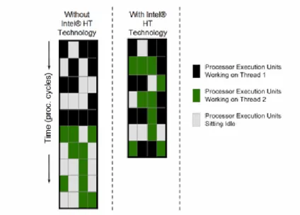
Modern superscalar processors can detect and exploit high levels of parallelism in the instruction stream, being able to begin execution of high number of instructions every cycle. They do so through a combination of multiple independent functional units and sophisticated logic to detect instructions that can be issued (sent to the functional units) in parallel. However, their ability to fully use this hardware is ultimately constrained by instruction dependencies and long-latency instructions limiting available parallelism in the single executing thread. The effects of these, as an example, are shown as vertical waste (completely wasted cycles) and horizontal waste (wasted issue opportunities in a partially-used cycle) in Figure 2.1, which depicts the utilization of issue slots on a superscalar processor and capable of issuing four instructions per cycle.
Multithreaded architectures employ multiple threads with fast context switching between threads. Fast context switches require that the state (program counter and registers) of multiple threads be stored in hardware. Latencies in a single thread can be hidden with instructions from other threads, taking advantage of inter-thread parallelism (the fact that instructions from different threads are nearly always independent).
51
Simultaneous Multithreading (SMT) and Intel’s implementation of it – Hyper-Threading (HTT), combines the superscalar’s ability to exploit high levels of instruction-level parallelism with multithreading’s ability to expose inter-thread parallelism to the processor. By allowing the processor to issue instructions from multiple threads in the same cycle, simultaneous multithreading uses multithreading not only to hide latencies, but also to increase issue parallelism. SMT and HTT can deal with both vertical and horizontal waste, as shown in Figure 2.2 and Figure 2.3.
Figure 2.1: Utilization of issue slots on a superscalar processor.
Figure 2.2: Utilization of issue slots on a superscalar SMT processor with 5 threads.
Figure 2.3: Utilization of issue slots on Intel’s Nehalem based processor with HTT.
51
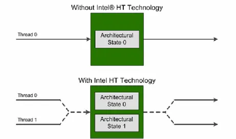
In Intel’s HTT the key hardware mechanism underlying this capability is an extra architectural state supported by the hardware [1]. Each thread in the processor is simply an instruction stream associated with a particular hardware context, as shown in Figure 2.4. Thereby each architectural state can support its own thread.
Figure 2.4: Intel’s HT Technology enables a single processor core to maintain two architectural states.
Many of the internal microarchitectural hardware resources are shared between the two threads. Operating systems and applications can schedule processes or threads on those logical processors. When one thread is waiting for an instruction to complete, the core can execute instructions from another thread without stalling. In addition, two or more processes can use the same resources. If one process fails then the resources can be readily re-allocated. The performance impact varies, depending on the nature of the applications running on the processors and on how the hardware is configured, but in most of the cases, Intel’s HTT and SMT allow substantial increase of the processor throughput, improving overall performance on threaded software.
51
2.2
The complexity of SMT
SMT processor is more complex than a corresponding single-threaded processor [8]. Potential sources of that complexity include:
Fetching from multiple program counters — following multiple instruction streams will either require parallel access to the instruction cache(s) and multiple decode pipelines, or a restricted fetch mechanism that has the potential to be a bottleneck.
Multiple register sets — accessing multiple register sets each cycle requires either a large single shared register file or multiple register files with a complex interconnection network between the registers and the functional units. In either case, access to the registers will be slower than in the single-threaded case.
Instruction scheduling — in considered SMT processors, the scheduling and mixing of instructions from various threads is all done in hardware. In addition, if instructions from different threads are buffered separately for each hardware context, the scheduling mechanism is distributed (and more complex), and the movement of instructions from buffers to functional units requires another complex interconnection network.
2.2.1 Complexity of Intel’s HTT
Intel processors can have varying numbers of cores, each of which can support two threads when Intel HT Technology is enabled [1]. For each thread, the processor maintains a separate, complete architectural state that includes its own set of registers as defined by the Intel 64 architecture [3] [5]. Some internal microarchitectural structures are shared between threads. Processors support SMT by replicating, partitioning or sharing existing functional units in the core. Hyper-threaded processor installed in our system under test has the following implementation policy [3][5]:
51
1. Replication — the unit is replicated for each thread.
register state
renamed RSB
large page ITLB
2. Partitioning — the unit is statically allocated between the two threads.
load buffer
store buffer
reorder buffer
small page ITLB
3. Competitive Sharing — the unit is dynamically allocated between the two threads.
reservation station
cache memories
data TLB
2nd level TLB
4. SMT Insensitive — all execution units are SMT transparent
2.3
Introduction to Queuing Networks
Since substantial part of the research work is dedicated to construction of appropriate SMT/HTT models, in this section some background information about Queuing Networks is provided to reader, which will help him to better comprehend the rest of the work.
2.3.1 Queuing Network
During many years, computer and communication systems have been studied as a network of queues [16]. According to [17] Queuing network modeling is a particular approach to computer system modeling in which the computer system is represented as a network of
51
queues which is evaluated analytically. A network of queues is a collection of service centers, which represent system resources, and customers, which represent users or transactions. Figure 2.5 illustrates a single service center. Customers or transactions arrive at the service center, wait in the queue if necessary, receive service from the server, and depart. In fact, this service center and its arriving jobs constitute a queuing network model.
Figure 2.5: Single service center.
Here there are some definitions of queuing networks used in the work:
Class: A class is a group of customers with each customer of that group having the same workload intensities (Ac, Nc, or N and Zc) and service demand (Sc,d). A class
MUST define the service demand (Sc,d) at each service center [17] [24].
Throughput: Throughput is the number of customers received service at service center in a unit of time. Usually it has notation Xk, where k is a service center [17]
[24].
Response Time: Response Time is the average time a customer spends at a service center and has notation Rk [17] [24].
System Throughput: System Throughput is the number of customers/transactions serviced by the system within a given period of time and has notation ∑ [17] [24].
Visits: Average number of visits at service center. Usually it has notation Vk, where k is a service center.
System Response Time: System Response Time is the sum time a customer spends at 11
51
each service center. ∑ , where is the average number of visits at station k [17][24].
Service center Utilization: Service center Utilization is a ratio between the busy time (the time a service center is being used) and the whole measured period. This ratio describes the extent of utilization of a service center. Utilization could be greater than 0, but should be less than 1. Therefore, 0.5 utilization means half of the device’s possible capacity is being used [17] [24].
Arrival Rate: Arrival Rate is the rate of customers/transactions at which they arrive arriving to a queue in a unit of time and has notation [17] [24].
User Think Time: Think Time represents the time a user spends before submitting a request/transaction and has notation Z [17] [24].
Queue Length: Service center Queue Length identifies a number of customers waiting for service in a specific queuing center and has notation [17] [24].
A Queuing Network can be open, closed, or mixed depending on its customer classes [13]:
Open Model: A Queuing Network is open if customers/transactions arrive from outside of the system. Arrival rate ( ) denotes arrival intensity.
Closed Model: A Queuing Network is closed if customers/transactions are generated inside the system (such as in a terminal system). In closed classes, the number of class c terminals (Nc) and think time for each class c terminal denote workload intensity
(Zc).
Mixed Model: Systems that have both open classes (external input) and closed classes [13].
51
2.4
Queuing Network Simulation
Simulation modeling is becoming an increasingly popular method for network performance analysis. Generally, there are two forms of network simulation [13]:
• Analytical Modeling • Computer simulation
Analytical modeling is conducted by a mathematical analysis that characterizes a network as a set of equations. The main disadvantage is its overly simplistic view of the network and inability to simulate the dynamic nature of a network. Thus, the study of a complex system always requires a discrete event simulation package, which can compute the time that would be associated with real events in a real-life situation. A software simulator is a valuable tool, especially for today’s network with complex architectures and topologies. Designers can test their new ideas and carry out performance related studies, thus freeing themselves from the burden of “trial and error” hardware implementations.
A typical network simulator can provide the programmer with the abstraction of multiple threads of control and inter-thread communication. Functions and protocols are described either by finite-state machine, native programming code, or a combination of the two. A simulator typically comes with a set of predefined modules and a user-friendly GUI. Some network simulators even provide extensive support for visualization and animation [13]. In this thesis the JMT tool [4] has been used to model and simulate the queuing network with Finite Capacity Region presented in Chapter 5.
51
2.5
Summary
Most of the time processor resources are underutilized due to the reasons discussed in the chapter. Low utilization leaves a large number of execution resources idle each cycle.
In this chapter we provided theoretical background for SMT and HT technologies and showed in theory that they can efficiently deal with stated above problem. We also showed that queuing networks is a powerful yet simple modeling instrument allowing representation of complex system by restricting modeling aspects only for truly relevant system details and omitting irrelevant ones. This valuable advantage of QN permits us to restrict our attention only on modeling of the processor subsystem and omitting direct representation of other system subparts, like disks or memory.
51
Chapter 3
State of Art in SMT/HTT
modeling
Current chapter presents two state of art QN models aimed at modeling SMT and HT technologies and some extensions for them.
3.1 SMT/HTT Model 1: Queuing Network Model
Authors from BMC Software propose a simple Queuing Network model [6] aimed at modeling a Hyper – Threaded processor architecture with a single core. They base their model on the fact that a hyper-threaded processor duplicates just some parts of the hardware (supporting extra architectural state), adding less than five percent to the chip size on the path from memory to CPU, but not the CPU itself [6].
This architecture allows for some parallel processing except at the actual instruction execution phase. That keeps the CPU itself busier at the moments of stalls, increasing the actual instruction execution rate [7]. Of course in order to take advantage of HTT, as with any multiprocessor system, multiple threads (in one or several processes) must simultaneously want access to a processor.
From the application’s point of view each job visits one of the two logical processors offered 15
51 to it by the operating system.
On the chip, each instruction execution goes through two phases. On the first one, an instance of the duplicated part of the hardware does preparatory work, looking up data and instructions in the cache or getting them from memory. And then the single real CPU executes the instruction.
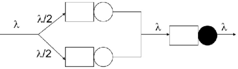
The situation is modeled thus with three queues shown in Figure 3.1. Jobs arrive to the system at the rate of per second and go to one of the two preparatory queues with probabilities p1 and p2, respectively. Since each job goes someplace, sum of p1 and p2 must be equal to one. Under assumption that OS has load balancing mechanism we can assume that p1 = p2 = 1/2.
Figure 3.1: Queuing network model of a single core processor with HTT and load balancing
On the Figure 3.1, the solid circle represents the single physical CPU core, and open circles are the places where the work is done prior to the instruction execution.
Supposing that service time at the preparatory queue is s1 seconds/job and the service time at the real CPU core is s2 seconds/job and that the job inter-arrival times and service times are exponentially distributed, the mean response time of an open Queuing Network models becomes [6]: (3.1) 16
51
With load balancing assumption p1 = p2 = 1/2, Response time (R) becomes:
(3.2)
In order to use model to predict system response time for real measured workload values λ, the parameters s1 and s2 need to be estimated. However there is a problem with parameters estimation, since the average total service time for each job, seen from the outside, can be measured but that does not tell anything about the internal service times, except that:
(3.3)
,
To validate the model authors ran a bon a single processor machine running at 2400 MHz Intel PowerEdge CPU. As a benchmark they use a self-made multithreaded Java application configurable to generate various kinds of compute intensive workloads.
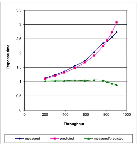
In order to test the model and to understand Hyper – Threading architecture, authors found the best fitting values of s1 and s2 for analyzed dataset. Those values turned out to be equal to s1 = 0.13 and s2 = 0.81 for the model on Figure 3.2. These values suggest that about 15% of the work occurs in the parallel “preparatory phase” of the computation, while instruction execution consumes about 65% [6]. Figure 3.2 show the results of the experiment and analysis.
51
Figure 3.2: Response Time curves for one-second job (single processor, HT on, predictions for model from Figure 3.1)
The fact that the measured data is fitted so well with reasonable parameter values suggests that the model is sound. Following section extends this model to take into consideration also dual core and quad core processors, that is, processors with two and four cores, respectively.
3.1.1 Model Extension
Unfortunately authors of the work do not extend their research on the technology for different processor types and propose model only for single core processor.
In our research, instead, we try to evaluate SMT and HTT performance effects for different system configurations, which certainly will result in more realist case usages and produce more comprehensive assessment of the technologies. Under changed system configuration we intend a different number of active CPU cores and different processor clock frequency. All
0 0,5 1 1,5 2 2,5 3 3,5 0 200 400 600 800 1000 R s ponse t im e Throughput
measured predicted measured/predicted
51
examined configurations are listed in detail in “Methodology” section of next chapter.
Finally, we tried to extend proposed model to reflect also system configurations examined in our work.
3.1.1.1 Extension 1: Dual core processor with HTT
Figure 3.3 illustrates an extension of previous model for dual core processor supporting HTT, or equivalently two-way SMT. The model is obtained simply by replication of the processor core, including all its instruction preparation and execution resources.
Figure 3.3: QN model for Dual core processor with HTT and optimal load balancing mechanism
On the Figure 3.3, the solid circles represent the execution units, and open circles are the places where the work is done prior to the instruction execution.
From the application’s point of view, now with active HTT each job visits one of the four logical cores offered to it by the operating system. As in previous case, on chip, each instruction execution goes through two phases. First, an instance of the duplicated part of the hardware inside one of two cores does preparatory work, looking up data and instructions in the cache or getting them from memory; and then the single real CPU executes the instruction
51 within the core.
The situation is modeled with six queues entering the service centers shown on the Figure 3.3, with three queues belonging to one core and remainder queues to another. Assuming perfect load balancing, jobs arriving to the system at the rate of per second then are directed to one of the two cores with equal probabilities, where they are further distributed to preparatory queues again with equal probabilities. Since each job goes someplace, the sum over all probabilities results to be one.
Again supposing that service time in four preparatory queues is s1 seconds/job and the service time at queues representing execution units is s2 seconds/job and that the job inter-arrival times and service times are exponentially distributed, the mean system response time of an open Queuing Network model from Figure 3.3 becomes:
(3.4)
With load balancing both between and inside cores ( ) the Response time becomes:
(3.5)
In order to use model to predict system response time for real measured workload values λ, the parameters s1 and s2 need to be estimated. Unfortunately, authors of the original model do not describe the way they estimated values of parameters s1 and s2, but just mention that they are the best fitting values.
In our case, optimal values estimation we use two-phase process based on error minimization. Under error we intend prediction error between dataset and model. First, we feed the model
51
with feasible s1, s2 parameter values found from the following set of equations:
(3.6)
Obtained in such way values of s1 and s2 are used to parameterize model, for which is then error estimated. Subsequently, this error is minimized using GRG Nonlinear solver, embedded in our tool used for processing, which always convergence to optimal values for all smooth nonlinear problems, which is also our case. Excessively, to ensure convergence to optimal values, another solving method – Evolutionary engine is applied. Obtained values are guaranteed to be optimal, thus producing lowest possible model prediction error.
3.1.2
Extension 2: Quad core processor with HTT
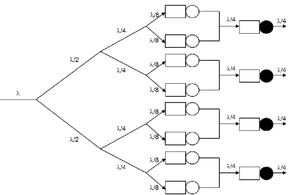
Figure 3.4 illustrates an extension for quad core processor supporting HTT. The model is again obtained by duplication of the processor core four times. The model characteristics remain the same as in case with Extension 1, but now OS recognizes eight virtual cores with active HTT.
Again assuming that operating system has working load balancing mechanism, the probability of request being processed by any of eight virtual cores is equal 1/8, thus the mean system response time of an open Queuing Network model from Figure 3.4 becomes:
∑ ∑ (3.6) 21
51
Figure 3.4: QN model for Quad core processor with HTT and optimal load balancing mechanism
With load balancing both between cores and inside core ( )
(3.7)
In order to use model to predict system response time for real measured workload values λ, the parameters s1 and s2 need to be estimated. The methodology remains the same as for Extension 1, with the only difference that initial (border) values of parameters s1 and s2 are obtained from the following equations:
(3.8)
51
Again, obtained parameter values are guaranteed to be optimal, thus producing lowest possible model prediction error.
3.2 SMT/HTT Model 2: Birth-Death Markov chain Model
3.2.1 Introduction
Author of the second model propose a Birth-Death Markov model targeted at modeling SMT enabled single core processor architecture having up to eight threads [8].
The key idea underlying is that SMT processor is best modeled as a load-dependent service center, while superscalar processor is easily modeled as simple service queue [8]. The same observation we use in our birth-death Markov chain model developed in Chapter 6, however with respect to this model we propose simpler model based only on two parameters and . The model we propose can be considered as a special case of this model.
A Markov chain model allows solving for system performance metrics derived from a probability distribution (produced by the model) on the queue population. This provides more accurate results for a load-dependent system such as the SMT processor than simpler queuing models that depend only on the average population in the queue.
Ordinary superscalar processor (superscalar represents the superscalar processor unmodified for SMT execution) is the M/M/1 queue, whose Markov model is shown in Figure 3.5.
Figure 3.5: The Markov state diagram for a single superscalar processor
51
The numbers in the circles are the population in the queue; the arcs flowing right are the rate at which jobs enter the system, and the arcs flowing left are the rate at which jobs leave the system.
The arrival rates for the superscalar processor on Figure 3.5 ( ) are all equal to a constant arrival rate ( . Because the throughput of the system is independent of the number of jobs in the system, the completion rates ( ) are all equal to a constant completion rate, ( ). The completion rate is assumed to be that of the unmodified superscalar processor found previously in their work.
A Markov system can be solved for the equilibrium condition by finding population probabilities that equalize the flow in and out of every population state.
Known values A and C, or for the most quantities , the well-known solution for M/M/1 system can be used.
The probability ( ) that k jobs are in the queue:
(3.8)
( )
Allows solving that zero jobs are in the queue:
(3.9)
∑
Thus the utilization (U) is the probability that there is more than one job in the system, and it is simply:
(3.10)
The average population (N) of the queue is:
51
(3.11)
̅ ∑
And the response time (R), from Little’s Law [17]:
(3.12)
̅
3.2.2
SMT processor model
Similar, but more complex Markov model for the SMT processor is shown on Figure 3.6, aimed at modeling a limited load-dependent server.
Figure 3.6: The Markov state diagram for single core eight-way SMT processor
It is similar to the M/M/m queue - a queue with multiple equivalent servers, however, in the M/M/m queue the completion rates vary linearly with the queue population when the population is less than , which is not true here. In this system on Figure 3.6, the completion rates are the throughput rates of non-modified superscalar processor ( ) multiplied by the factor which depends on queue population. The completion rate figures have been obtained by the authors after simulation performed on SMT processor.
For example, when there is only one job in the system, the SMT processor runs at 0.98 times the speed of the superscalar, but when five jobs are in the system, it completes jobs at 2.29 times the speed of the superscalar. That is, while the job at the head of the queue may be
24 25
51
running more slowly, because all five jobs are actually executing the completion rate is higher, proportional to the throughput increase over the superscalar.
Another assumption - the rate of completion is constant once there are more jobs than thread slots in a system. This assumes that the cost of occasionally swapping a thread out of the running set (an operating system context switch) is negligible. This is the same assumption to use a single completion rate for the superscalar model. This assumption favors the superscalar, because it incurs the cost much earlier (when there are two jobs in the running set).
Because the arrival rate is still constant, but the completion rates ( ) are not, the formula for the probability of population k is:
∏
(3.13)
For the simulation results, this series becomes manageable because the tail of the Markov state diagram is once again an M/M/1 queue. So,
(3.14) { ∏ Where M = (0.982) (1.549) … (2.425) (2.453).
As with the M/M/1 queue, because all probabilities sum to one and we can express all probabilities in terms of p0, we can solve for p0, and thus the utilization.
We can solve it because the sum of all probabilities fork is a series that reduces to a single term (as long as A/2.463C < 1), as does the M/M/1 queue when A/C < 1, thus:
(3.15)
51
( ) ( )
In order to calculate response times, first we need to know the average population in the queue: (3.16) ̅ ∑ ∑ ∑ (3.17) ̅ ∑
Response time can then be computed from the average population and the jobs arrival rate ( ) using Little’s Law [17]:
(3.18)
̅
Unfortunately, author of the model does not provide any validation approach. The validation results of our model, which can be considered as a special case of this model, are represented in Chapter 6.
51
Chapter 4
Potential of SMT / HTT
In this chapter we perform experimental validation of the SMT and HTT theoretical aspects discussed previously in Chapter 2. Also we perform a series of benchmark runs to reveal true performance impacts enabled by Simultaneous Multithreading and Hyper-Threading Technology for different system configurations using two types of benchmarking suite.
4.1
Performance Claims
The advantages of hyper-threading are listed as improved support for multi-threaded code, allowing multiple threads to run simultaneously; increased throughput and reduced response time. According to Intel, its first implementation only used five percent more die area on chip comparing to equivalent non-hyper threaded processor, but the performance increase was 15 – 30% greater [2][11]. For a previous generation processors Intel claims up to a 30% performance improvement compared with an otherwise identical, non-simultaneous multithreading processors [2][10][11].
According to [10], in some cases a previous generation Pentium IV processor running at 3 GHz clock frequency with HT activated can even beat a Pentium IV running at 3.6 GHz with HT turned off. Intel also claims significant performance improvements with a HTT in some artificial intelligence algorithms.
51
Technology improves throughput and efficiency for better performance and performance per watt. Intel HT Technology provides greater benefits in Intel Core i7 processors, and other processors based on the Nehalem core including the Xeon 5500 series of server processors than was possible in the Pentium 4 processor era when it was first introduced [12]. The discussion in [12] refers to Intel 64 architecture, with particular emphasis on Intel processors based on the Nehalem core including the Core i7 Processor and the Xeon 5500 series of processors. According [12] the performance improvement for this workload is 30% (1.30x) when Intel HT Technology is enabled for the workload consisting mostly of integer ALU operations. The response time as viewed by the client dropped from 50 ms per transaction to 37 ms per transaction with Intel HT Technology enabled (about 26%).
4.2
Test bed configuration
The system under test used for benchmarking has Intel Core i7 920 processor and 12 GB of DD3 DRAM installed. The processor is characterized by 4 cores, default clock speed of 2.66 GHz, HT Technology and three eight-byte DD3 channels. Processor cache memory has following characteristics [5]:
o 1st
level instruction cache: 32 KB per core 4-ways o 1st
level data cache: 32 KB per core 8-ways (write-back) o 2nd
level data cache: 256 KB per core o 3d
level data cache: 8 MB per four cores shared across all cores
4.3 Methodology
To achieve a fairly comprehensive assessment of SMT/HTT, the evaluation has been performed for different system configurations. Since the key component of the system, which we try to model, is a processor, using a small self-made java program we were able to alter
51
processor states. In total, performance impact of Intel’s HTT has been evaluated for all the following system configurations:
4 cores, HT enabled, 2660 MHz 4 cores, HT enabled, 1596 MHz 2 cores, HT enabled, 2660 MHz 2 cores, HT enabled, 1596 MHz 1 core, HT enabled, 2660 MHz 1 core, HT enabled, 1596 MHz
2660 MHz is a maximum reachable clock frequency that a processor can have, and 1596 MHz is a lowest frequency that can be set for a processor. The choice of “border” frequencies is not accidental and it is intended to reveal the most productive technology usage cases and to understand how drastic changes in the processor clock frequency affects the performance gain enabled by SMT/HTT technology. Additionally, the configurations listed above represent of the most encountered computer systems.
4.3.1 Obtain system measures
Next, for each examined system configuration, representing changed processor state, the system needs to be measured under certain workloads to obtain workload and performance measures.
Subsequently, in Chapter 6, this data will serve as an input for SMT/HTT models evaluation step and obtained model performance indices will be compared to the measured system outputs.
51
4.3.2 Benchmarking
Benchmarks are used to generate workload and record both workload and performance metrics. In computing, a benchmark is the act of running a computer program, a set of programs, or other operations, in order to assess the relative performance of a system, normally by running a number of standard tests and trials against it, accordingly, the workload and performance measures are strictly dependent on the type of benchmark and on each benchmark run or trial itself. In our research we use two different benchmarking suites to assess SMT/HTT performance, each having its own measuring approach and features.
4.3.3
SPEC Power SSJ 2008
First benchmark used for evaluations is SPEC Power SSJ 2008. It is a product developed by the Standard Performance Evaluation Corporation (SPEC) and it is the first industry standard for measuring both performance and power consumption of computer systems [18].
SPEC benchmark allows estimation of such performance measures, like system throughput and processor utilization, but unfortunately does not provide any suitable means to obtain system response time.
At a high level benchmark models a server application with a large number of users [19]. Requests from these users arrive at random intervals (modeled with a negative exponential distribution), and processed by a finite set of threads of the server. The exponential distribution may result in bursts of activity; during this time, requests may queue up while other requests are being processed. The system will continue processing transactions as long as there are requests in the queue.
The whole benchmark suite consists of three main components [18] [20]:
Server Side Java (SSJ) Workload: SSJ Workload is a Java program designed to exercise the CPU(s), caches, memory, the scalability of shared memory processors, JVM (Java Virtual Machine) implementations, JIT (Just In Time) compilers, garbage
51
collection, and other aspects of the operating system of the system under test (SUT).
Power and Temperature Daemon (PTDaemon): The PTDaemon is to offload the work of controlling a power analyzer or temperature sensor during measurement intervals to a system other than the SUT.
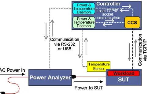
Control and Collect System (CCS): CCS is a multi-threaded Java application that controls and enables the coordinated collection of data from multiple data sources such as a workload running on a separate SUT, a power analyzer, and a temperature sensor. It also includes Visual Activity Monitor (VAM) - software package designed to display activity from one, two, or three SUT‟s simultaneously, in combination with the SPECpower_ssj2008 benchmark.
In experiments the whole system has been configured without PTDaemon component because of non-availability of the required equipment, and secondly, because eventually the goal is to understand performance and not power impact enabled by the technology.
Figure 4.1 illustrates the architecture of a standard SPECpower_ssj2008 benchmark implementation including Power Analyzer and Temperature sensor components, which in our case are omitted for the reasons listed above.
Figure 4.1: Architecture of a s SPEC Power SSJ 2008 benchmark implementation
51
4.3.3.1
SPEC’s Server Side Java (SSJ) Workload
The SSJ Workload is a component responsible for benchmark workload generation. First, the system needs to be calibrated. The calibration phase is used to determine the maximum throughput that a system is capable of sustaining. Once this calibrated throughput is established, the system runs at a series of target loads. Each load runs at some percentage of the calibrated throughput. By default, 3 calibration intervals are used, each four minutes long. The calibrated throughput (used to calculate the target throughputs during the target load measurements) is calculated as the average of the last 2 calibration intervals.
For compliant runs, the sequence of load levels decreases from 100% to 0% in increments of 10%. At each load level the system is measured for 120 seconds. The intervals between load level measurements, the so-called “warm-up” and “cool-down” are equal to 30 seconds. Measuring the points in decreasing order limits the change in load to 10% at each level, resulting in more stable performance measurements. Using increasing order would have resulted in a jump from 100% to 10% moving from the final calibration interval to the first target load, and another jump from 100% to Active Idle at the end of the run.
4.3.4 A synthetic benchmark
On the system under test (SUT) we run a simple web application written in Java (a *.war file) deployed on Apache Tomcat webserver. This application is composed of a single page which performs a computation on floating point numbers and stresses both the CPU and memory hierarchy. The service time of this page is exponentially distributed.
To load the system we use a multi-threaded load generator that generates http requests with exponentially distributed inter-arrival times. The load generator runs on a separate machine connected with the system under test by 100 MBits/s network connection to avoid network bottlenecks.
The advantage of using the load generator and a synthetic workload is that we can create a
51
load which can be easily modeled, e.g., exponential inter-arrival times and exponential service-times. Moreover, the load generator besides processor utilization can also measure system response time, so that we can analyze not only the utilization and throughput, but also the response time.
4.3.4.1 Synthetic Workload
The crucial points of workload can be listed as:
Time complexity for the processing of one request should be O(n)
The workload should stress the memory hierarchy
Partially memory and partially CPU bound
Possibility to tune impact of memory accesses
The workload consists of two phases: initialization phase and actual execution phase. At initialization phase a working set of vectors and a filter vector of length are generated. Each vector has a random length uniformly distributed between and .
At execution phase a random vector is selected and two vectors and of length n are allocated. Then vector is filled with sums of p random strides of length w from v and convolved with filter vector Convolution result is stored in . Finally the sum of the elements in is returned.
Summarizing, execution phase consists of three main steps having complexity O(n): 1. Filling the source vector a
2. Compute b performing the convolution of a and f 3. Sum the elements of b
There are some cache size considerations which must be met for optimal workload generation. The memory used by the working set vectors should exceed the size of the LLC (Last Level Cache), that is to say:
51
( ) (4.1)
Source and destination vectors and should fit in a private cache L1 or L2:
(4.2)
Filter vector must fit in the first level cache:
(4.3)
Figure 4.2 demonstrates the process of filling the source vector with number of strides each having length :
Figure 4.2: Synthetic workload: Filling source vector
For small w, a full cache line is read but not used; the prefetcher helps only for large w.
Figure 4.3 demonstrates the convolution process for obtained source vector a with filter vector
f; the results is stored in destination vector b:
51
Figure 4.3: Synthetic workload: Convolution process between source vector a and filter vector f
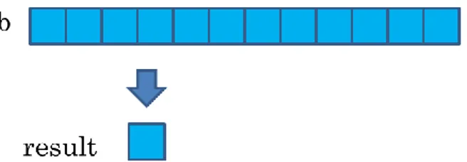
Finally, Figure 4.4 how the result value is obtained:
Figure 4.4: Synthetic workload: Result calculation
In our benchmark runs to generate optimal workload the values of p, w and n have been defined adhering to defined above observations and are equal to 20, 32 and 10000, respectively.
4.3.4.2 IronLoad Generator
IronLoad generator is used to generate benchmark workload and able of capturing such performance measures like processor utilization and system response time. For each system configuration listed in Section 4.3 the benchmark run is performed. Each benchmark run consists of two main phases: maximum throughput estimation that system is capable of sustaining for closed loop and run at series of target loads. Each load runs at some percentage of target utilization. If utilization is I, then target load is equal to:
(4.4)
For compliant runs the sequence of target utilization load levels decreases from 80% to 5% in increment of 5%, in total resulting in 16 load levels. Load level duration is set to be 1200
51
seconds and interval between load levels is equal 30 seconds. All the measured data is saved in CSV format.
4.4
Performance results
The following performance data have been obtained after a series of benchmark runs for System Throughput, Processor Utilization and System Response Time.
The Response Time measure is available only for synthetic benchmark, since SPEC Power SSJ 2008 does not provide ant suitable means get this measure. Feasible values for Utilization vary in range from 0 to 100%.
Each plot illustrates performance data obtained at specific CPU clock frequency for all examined combination of cores.
4.4.1 System Throughput
System Throughput is estimated as number of operations performed in a second. The measurement results are available for both synthetic and SPEC Power benchmarks.
Estimated performance gain enabled by HTT over the equivalent system configuration but without HTT, is indicated in the right upper corner of each plot and it is strictly related to the value of parameter Alpha, calculation of which is discussed in the corresponding section of next chapter:
51
4.4.1.1
SPEC Power SSJ 2008 benchmark
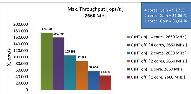
Figure 4.5: System Throughput with HT {on, off} for {4, 2, 1} cores at 2660 MHz
Figure 4.6: System Throughput with HT {on, off} for {4, 2, 1} cores at 1596 MHz
SPEC Power benchmark exhibits significantly higher performance increase range. Depending on the configuration, throughput increase varies from 9 to 33%. Again, greater increment is achieved at “weaker” configurations.
175.120 160.409 105.868 87.453 57.858 43.488 0 20.000 40.000 60.000 80.000 100.000 120.000 140.000 160.000 180.000 200.000 X, ops /s
Max. Throughput [ ops/s ]
2660 MHz X (HT on) [ 4 cores, 2660 MHz ] X (HT off) [ 4 cores, 2660 MHz ] X (HT on) [ 2 cores, 2660 MHz ] X (HT off) [ 2 cores, 2660 MHz ] X (HT on) [ 1 core, 2660 MHz ] X (HT off) [ 1 core, 2660 MHz ] 4 cores: Gain = 9,17 % 2 cores: Gain = 21,06 % 1 core: Gain = 33,04 % 117.535 103.824 68.238 58.425 38.120 28.760 0 20.000 40.000 60.000 80.000 100.000 120.000 140.000 160.000 180.000 200.000 X, ops /s
Max. Throughput [ ops/s ]
1596 MHz X (HT on) [ 4 cores, 1596 MHz ] X (HT off) [ 4 cores, 1596 MHz ] X (HT on) [ 2 cores, 1596 MHz ] X (HT off) [ 2 cores, 1596 MHz ] X (HT on) [ 1 core, 1596 MHz ] X (HT off) [ 1 core, 1596 MHz ] 4 cores: Gain = 13,21 % 2 cores: Gain = 16,80 % 1 core: Gain = 32,55 % 38
51
4.4.1.2
Synthetic benchmark
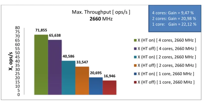
Figure 4.7: System Throughput with HT {on, off} for {4, 2, 1} cores at 2660 MHz
Figure 4.8: System Throughput with HT {on, off} for {4, 2, 1} cores at 1596 MHz
Experiment data reveals that for synthetic benchmark throughput gain varies from 9 to 22% depending on the configuration of the system. Interestingly, gain ration is preserved for different frequencies, except for configuration with 4 cores. Maximum gain (in relative terms) is achieved at “weaker” configurations.
71,855 65,638 40,586 33,547 20,695 16,946 0 5 10 15 20 25 30 35 40 45 50 55 60 65 70 75 80 X, ops /s
Max. Throughput [ ops/s ]
2660 MHz X (HT on) [ 4 cores, 2660 MHz ] X (HT off) [ 4 cores, 2660 MHz ] X (HT on) [ 2 cores, 2660 MHz ] X (HT off) [ 2 cores, 2660 MHz ] X (HT on) [ 1 core, 2660 MHz ] X (HT off) [ 1 core, 2660 MHz ] 4 cores: Gain = 9,47 % 2 cores: Gain = 20,98 % 1 core: Gain = 22,12 % 50,137 42,619 25,275 20,925 13,1 11,15 0 5 10 15 20 25 30 35 40 45 50 55 60 65 70 75 80 X, ops /s
Max. Throughput [ ops/s ]
1596 MHz X (HT on) [ 4 cores, 1596 MHz ] X (HT off) [ 4 cores, 1596 MHz ] X (HT on) [ 2 cores, 1596 MHz ] X (HT off) [ 2 cores, 1596 MHz ] X (HT on) [ 1 core, 1596 MHz ] X (HT off) [ 1 core, 1596 MHz ] 4 cores: Gain = 17,64 % 2 cores: Gain = 20,79 % 1 core: Gain = 17,49 % 39
51
4.4.2 Processor Utilization
Measurement of processor utilization can be very misleading. Generally, multi-core systems present a reporting dilemma to the measurement community [6]. For example, when both processors on a dual processor machine are active during an interval is the utilization 100% or 200%? To eliminate the ambiguity, the number of processors for which the utilization is reported has to be specified and a performance measurement tool must use one convention consistently and make clear how its output is to be interpreted.
For a hyper-threaded processor, which is a single physical CPU designed to appear to the operating system and its measurement tools as two separate cores, the problem is even more compounded. Since hyper-threading is in principle transparent to the operating system and applications, existing measurement tools need no modifications to run in a hyper-threaded environment [6]. But what will they report for processor Utilization – the answers vary.
Traditional way is to define utilization as a fraction of utilized threads. In the case with HTT on number of available to the system threads doubles, hence resulting in lower utilization. Below there is a series of plots for utilization measured for different system configurations using SPEC Power SSJ 2008 benchmark and a synthetic benchmark.
As a reader can notice from Figures 4.10 – 4.13 and figure from Motivation section, utilization curves with HTT off are straight lines for all system configurations. This fact can be easily described by Utilization law [17][24], which represents linear relationship between utilization and workload:
(4.1)
where dCPU is a service demand. In fact, for configurations with HTT off, according to plots
utilization scales linearly with workload. However, the situation changes in the presence of SMT (Figures 4.10 – 4.13) and the growth becomes nonlinear.
There are several research papers focusing on service demand estimation under the
51
assumption that Utilization law holds. As an example parameter dCPU can be estimated on
some data samples using Utilization law, by measuring U and X for some intervals. The resulting U versus X must be reported on a chart. Since we have linear dependence we can find the line that better approximates obtained U versus X samples using Linear Regression estimation. The slope of the line would represent service demand (dCPU).
Figure 4.4 illustrates example of dCPU calculation for the SPEC Power dataset. In example
below erminology and notation details can be found in Chapter 2.
Figure 4.9: Service demand (d) estimation for SPEC Power benchmark data samples at 4 cores, 2660 MHz wit HT configuration
90,70957447 73,35659574 60,01887324 48,8693617 39,13382979 32,02673759 25,29169014 18,32489362 12,44471831 6,707253521 0,319731801 0 10 20 30 40 50 60 70 80 90 100 0 25.000 50.000 75.000 100.000 125.000 150.000 175.000 200.000 U( sa r) [ % ] Target X [ ops/sec ] Service demand (dCPU) estimation
UCPU = 0,0005*X + 5,5361