Contents
Introduction……….5
1 Evaluation of Active Labor Market Programs in Romania 1.1 Introduction………7
1.2 Administration of Labor Programs………8
1.2.1 Labor Redeployment Program……….9
1.2.2 Program Goal……….9
1.3 Active Labor Market Policies……….10
1.4 Did ALMPs make any difference?...11
1.5 Data Collection……….13
1.6 Structure of the Sample………..14
1.6.1 The group of participants……….14
1.6.2 The group of non-participants……….……….15
1.6.3 Background characteristics……….16
1.7 Evaluation of the Program Impact………..18
1.7.1 Definition of basic notation……….19
1.7.2 The choice of the causal parameter of interest and the estimator………21
1.7.3 Selection bias……….21
1.7.4 Propensity score matching……….………….22
1.8 Which Variables have Most Effect on the Participation Process?...26
1.9 Results……….27
2 Bootstrap Methodology: Does It Always Work? 2.1 Introduction……….29
2.2 The Bootstrap Methodology………31
2.3 Can We Talk About One Type of Bootstrap?...32
2.3.1 The non-parametric procedure………32
2.4 Errors in Bootstrap………33
2.5.1 Consistency of the resampling methods……….……….………34
2.5.2 Asymptotic acuracy……….……….35
2.6 Failure of Bootstrap Methods……….…………..36
2.6.1 Problem setting……….36
2.6.2 Bootstrap variance vs Abadie-Imbens variance……….37
2.7 What About the Bootstrap Variance and Kernel Matching?...39
3 Monte Carlo Simulation 3.1 Introduction……….…………43
3.2 The choice of the Sample……….…………44
3.3 Generating Distributions………..45
3.3.1 Data generating process………47
3.3.2 Generating distribution of ATT……….49
3.3.3 Generating distribution of bootstrap estimator………..49
3.3.4 Generating distribution of Abadie-Imbens estimator…………50
3.4 Computational Aspects………..50 3.5 Results……….50 Conclusions...59 Appendix………61 Bibliography...83 Acknowledgements...85
“I zdrobi lazne dijamante ko ljusku supljeg oraha nek bulevari sveta pamte muziku tvojih koraka” Dj. Balasevic
(And crush the fake diamonds like an empty walnut shell - Let boulevards of the World remember the music of your steps…)
Introduction
The project, in which I participated as an Erasmus student in Autonomous University of Barcelona, focused on estimation of the effects of active labour policies implemented in Romania in 1999 and I collaborated with Dr. Nuria Rodriguez Planas, who was one of the coordinators of the project. The title of the paper that originated from the research, published by IZA (Institute for the Study of Labour) in May 2006 and revised in May 2007, is “Evaluating the Active Labour Market Programs in Romania”1. In what follows, I will refer to this paper by Rodriguez-Planas and Benus (2006)
The objective of the research was to quantify the effects of Active Labour Market Policies introduced in Romania in the late nineties and targeted to the unemployed. The effects are retrieved from a suitable comparison between the participants of at least one of the labour programs and those who continued to search for a job as openly unemployed, without applying to any service offered by the program.
My contribution to the paper was a continuous work as a research assistant to Dr. Rodriguez Planas. I contributed to the construction of the variables, to the analysis of the descriptive statistics and the estimation of the effects of the policies using alternative methodologies, such as OLS and propensity score matching techniques.
The remainder of this thesis is organised as follows. Throughout the Chapter 1 I will build upon part of the work that I did to contribute to the
1
paper Rodriguez-Planas and Benus (2006), summarise the main findings and describe the methods that we used to come out with meaningful estimates of the causal parameter of interest. In the Chapter 2 I will introduce the basic bootstrap theory and discuss some practical problems related to statistical inference when using the bootstrap methodology for matching estimators, referring to the article Abadie and Imbens (2004). Finally in Chapter 3, I will guide the reader through the Monte Carlo approach of generating data and the construction and comparison of the distributions of bootstrap and Abadie-Imbens estimators for the variance of matching estimator for the treatment effect. In order to investigate upon the presence of a significant difference between the estimators across the different matching methods, Monte Carlo simulation was done in three different contexts of matching on propensity score: kernel, nearest neighbour and nearest neighbour with caliper matching.
Chapter 1
Evaluation of Active Labor Market Programs in Romania
1.1. INTRODUCTION
After the fall of the government of Ceausescu in December 1989, Romania was headed towards the market economy. After 40 years of central planning, the road to transition was a process which brought up very high social costs, one of which was high unemployment rate.
Unemployment figures talk by themselves: from almost no unemployment before 1990, to almost 12 percent in 1999. In an attempt to minimize the social costs of transition, the Romanian government initially hesitated to impose tight fiscal constraints and passive labour policies were generally preferred in the early 1990’s. In the late 1990s, attempts to impose macroeconomic stability without full structural support led to negative economic growth and to an increase of the poverty rate from 20 percent in 1996 to 41 percent in 1999.
In 1995 the government of Romania signed the Loan Agreement for the Employment and Social Protection Project with the World Bank, which consisted in:
• Flexible adult training systems
• Reforms in social insurance and assistance projects
In terms of policies undertaken, passive labour policies were continued to be implemented, and the concretization of an urgent necessity for active approach to labour policies took place.
The research undertaken by Rodriguez Planas and Benus (2006) was done in collaboration with the Romanian Ministry of Labor and Social Protection and the National Agency for Employment and Vocational Training, while the whole project of introduction of labor policies was funded by the World Bank Employment and Social Protection Project.
The contents of the following sections in this chapter are largely built upon the work by Rodriguez Planas and Benus (2006), to which the interested reader is referred for more specific details about the implementation of the programs.
1.2 ADMINISTRATION OF LABOR PROGRAMS
The Ministry of Labor and Social Protection (MOLSP) was in charge Romania’s labor programs and its implementation went through the establishment of the network of local offices on the national level. In each of the 40 regions (so-called “judet”) there was established a main office and several branch offices – summing up to 200 offices throughout the country.
Employment services at these local offices have gradually improved over the past few years. Much of this improvement has taken place since 1995 when the Romanian Government signed a Loan Agreement for the Employment and Social Protection Project. The project provides financial and technical support to the MOLSP efforts to:
• strengthen the capacity of labor offices to administer increasing number of claims for unemployment benefits and active labor adjustments services;
• develop a flexible adult training system which responds to evolving labor market demand resulting from economic restructuring;
• implement reforms in social insurance and assistance programs, targeting those population groups that are most vulnerable.
Employment and Social Protection Project funds have also been used to support the Labor Redeployment Program (LRP in what follows), a program designed to reduce the negative economic and social impact of enterprise privatization, restructuring, and liquidation by offering services to displaced workers.
1.2.1 The Labor Redeployment Program
The LRP program was designed in 1997 to address mass labor displacements resulting from privatization and economic reform. The design of the LRP was enhanced by inputs from foreign experts - from the World Bank and the U.S. Department of Labor. Financing for the program came from the World Bank European Social Protection Program, the Romanian Unemployment Fund and U.S. Department of Labor through the US Agency for International Development.
The lead agencies in developing Active Labor Market Programs in Romania (ALMPs in what follows) are the MOLSP and the National Agency for Employment and Vocational Training. Together, these agencies have put in place the targeted ALMPs currently operating in Romania.
1.2.2 Program Goal
The primary goal of the LRP is to reduce the negative economic and social impact of privatization, restructuring, and liquidation of Romanian enterprises during the period of economic reform and privatization. To achieve this goal, the LRP offers services to support the reintegration of displaced workers into the workforce in the shortest time possible. The program also seeks to support the creation of new jobs and to preserve existing jobs, thus contributing to economic growth.
1.3 ACTIVE LABOUR MARKET POLICIES
ALMPs are defined as interventions that are directly targeted at the unemployed and are designed to raise employment. Conventional theory defines these policies as:
• Job broking activities with the aim of improving equilibrium between vacancies and unemployed;
• Labour market training; and • Job creation activities.
The programs were adopted and launched on a large scale only in 1997. The design and implementation of Romania’s ALMPs are partially funded by the World Bank Employment and Social Protection Project (ESPP), whilst the administration of labour programs was launched by Romanian Ministry of Labour and Social Protection (MOLSP).
There were six ALMP’s defined at the beginning of 1997, out of which the first four were fully implemented on the large scale, and the last two were only partially introduced and delayed because of the lack of legal framework. These programs are:
1) Training and Retraining Services (TR in what follows) – candidates received up to nine months of training as well as a small subsistence salary. The cost of training was limited to $560 U.S. dollars per unit. Another requirement of this service was that local service providers must agree to achieve a minimum negotiated job placement rate and to show evidence of demand for trained workers.
2) Small Business Consulting and Assistance Programs (SB in what follows) – Displaced workers who start or operate a small business are eligible to receive legal, marketing, sales, financial services and consulting services. There are also provisions for short-term working capital loans of up to $25,000 U.S. dollars to program participants.
3) Public Service Employment (PW in what follows) – Local governments and other eligible organizations could propose public works projects with a maximum cost of $50,000 U.S. dollars (or higher with a no-objection from the World Bank). These public works projects covered the cost of supervisory personnel and up to 6 months of salary, where salary was set at the maximum of the average wage level of the type of activity provided.
4) Employment and Relocation Services (ER in what follows) - which included job and social counselling, labour market information, job search assistance, job placement services, and relocation assistance. The eligible candidates receiving relocation assistance were to be refunded for expenses of moving to another community (up to $500 U.S. dollars equivalent in lei). In addition, the program offered up to two months of salary at the minimum wage.
5) Small Business Incubator Assistance Programs – This program was designed to provide facilities, technical assistance, shared services and short-term working capital for new small businesses.
6) Local Economic Development Planning Services – This program was designed to support the cost of local economic assessments, workshops, studies and promotional materials.
1.4 DID ALMP’S MAKE ANY DIFFERENCE?
In order to provide a credible answer to this question, MOLSP together with the National Agency for Employment and Vocational Training (ANOFM) requested and funded the research, which was finally summarized and evaluated by Nuria Rodriguez Planas (Universitat Autònoma de Barcelona) and Jacob Benus (Impaq International).
The purpose of the study was to quantify, define and classify the effects of ALMPs introduced in Romania, where the particular entity of interest was the
effect on the population of the unemployed workers who took part in one of these programs. In fact, the main question was if the participants of any of the fully implemented programs were any better of at the time of the survey respect to those who continued to search for a job as openly unemployed, in terms of current state of employment and salaries.
The attention of the research was the population of the unemployed workers who registered in the Employment Bureau during 1999, and decided to participate or not participate in one out of four ALMPs. The motive that the individuals who were registered at the Bureau before 1999 were excluded from the study was a doubt that certain procedures regarding the programs were not entirely followed, because of the local lack of acquaintance with such programs. On the other hand, the individuals who took part in ALMPs in the period after 1999 were also out of the focus because too close to the survey time (year 2003) and it was considered that the impacts on the participants were not fully reflected.
The expected effects which represent the outcomes of interest were:
• Prospective of employment and higher salaries in the period soon after participation in one of the labour programs
• Prospective of employment and higher salaries further in future from ALMPs.
The sequence of events regarding the participation ad survey on ALMPs is illustrated in Figure 1.1.
Figure 1.1: Time Sequence of Events
1997 1998 1999 2000 2001 2002 2003
The first unemployed workers participate in ALMP’s Target population registers at the EB Survey time
1.5 DATA COLLECTION
The institute in charge of data collection was an outside Romanian firm called the Institute of Marketing and Polls. Using only the administrative Employment Bureau fonts of data would result in the lack of many precious information, especially the ones related to the wage history of the individuals. The data collection and the follow-up survey were specially designed for this research.
The questionnaires were submitted in 2002 to both participants and non participants who were registered at the EB in 1999. Hence, when talking about evaluation of the effects of the program, it is referred to ALMP services offered during this particular year. Moreover, Small Business Incubators assistance program and Local Economic Development Planning Services were not taken into consideration because, as explained before, not fully implemented on a large scale.
The data was collected from questionnaires which were submitted to the unemployed workers in January and February of 2002. The individuals were asked questions on employment and earnings at the survey time, during the years 2000 and 2001 and finally on employment and earnings during 1998 (before participation into ALMP). (see Appendix 1 for Chapter 1)
A random sample of 3999 individuals was drawn from the population of interest (see the illustration bellow), limited to 15 Romanian counties (judet) which are estimated to contain 86 percent of the total number of workers registered on the national level at EB, and are a representative image of the economy in Romania.
Figure 2. The target population and the sample
1.6 STRUCTURE OF THE SAMPLE
1.6.1 The group of participants
Any individual registered at the EB and voluntary took part in any of the four ALMP (Training and Retraining, Small Business assistance, Public Work Employment and Employment and Relocation program), and completed the program was considered as a participant .Taken in consideration 14 judet, 10 percent of the participants of each one out of four programs were randomly taken to obtain this stratified sample. The only exception was Training and Retraining program, where 25 percent of the population were taken because there was a very limited number of the participants to this program.
The final sample of participants considered counted 2047 individuals, where individuals with missing data, regarding any of the baseline or outcome related variables, being excluded. The percentage of excluded individuals because of the missing data problem was less than 5 percent, and hence regarded not a threat for the validity of results.
1.6.2 The group of non-participants
In order to select a representative sample of the population who seek for a job as openly-unemployed it was first determined, for each of the four ALMPs, the number of participants that were selected for the participant sample in each of the 15 judet. Next, in each county and for each ALMP, an equal number of non-participants were randomly selected from the Employment Bureau register list, where the non-participants were defined as those who did not participate in any of the four ALMP’s, but only registered as unemployed in EB. The final sample size of potential comparison group was 1501 (individuals with missing data being excluded from the sample).
Table 1.1 summarises the sample size by participation status and by program for each judet, while the Table 1.2 shows the number of participants of each program.
Table 1.1 : Number of individuals per judet and participation status
judet Non
participants Participants Total
1 (Alba) 83 83 166 2 (Bacau) 100 104 204 3 (Botosani) 72 72 144 4 (Buzau) 56 56 112 5 (Cluj) 145 143 288 6 (Dolj) 82 81 163 7 (Giurgiu) 12 12 24 8 (Gorj) 132 129 261 9 (Henedoara) 274 232 506 10 (Maramures) 71 71 142 11 (Neamt) 130 143 273 12 (Sibiu) 618 759 1,377 13 (Suceava) 106 87 193 14 (Vaslui) 68 78 146 Total 1,949 2,050 3,999
Table 1.2 : Number of individuals per each ALMP and participation
PROGRAM Frequency Percent
Training and Retraining 97 2.43
Small Business Assistance 447 11.18
Public Employment 555 13.88
Employment and Relocation services 951 23.78
Non Participation 1949 48.74
TOTAL 3999 100.00
1.6.3 Background characteristics
Rich background information was collected for each individual: demographic characteristics followed by employment, unemployment, and training experiences during 1998 . Relative frequencies in percentage points of each characteristics are presented in Table 1.3.
Considerable heterogeneity could be observed among different ALMP participants. It could be supposed that either the operators may be consciously selecting those individuals with a comparative advantage for the different ALMP programs, or individuals self-select into the different programs, basing their decision on personal experience, motivation or information available. For example, highly educated workers with more stable employment history had a tendency to participate in Small Business Consultancy and Assistance, whereas the youngest and those with the highest training predisposition participate in Training and Retraining. Male participants are more likely to enter a PW program while female ones are more likely to enter an ER program.
Even the comparison between non-participants and participants reflects that the latter seem to have had more stable employment history before attending the ALMP. Furthermore, their employment history was most similar to that of SB participants, whereas the age and education distribution of non-participants resembles that of ER non-participants. Two thirds of non-non-participants were male.
Table 1.3 Pre-Program Descriptive Statistics According to Participation Status (Percentages except where noted)
Training and Retraining (1) Small Business Assistance (2) Public Employment (3) Employment and Relocation Services (4) Non-participants (5) CHARACTERISTICS Male 45.83 50.69 89.89 45.92 63.82 Age 39.68 41.66 40.20 42.58 42.25
Less than 31 years old 5.56 4.99 13.03 7.50 8.93
Between 31 and 35 years old 27.78 22.71 19.33 14.59 16.46 Between 36 and 45 years old 47.22 40.44 38.43 40.16 36.58 Between 45 and 50 years old 15.28 17.73 18.20 20.62 19.79
More than 50 years old 4.17 14.13 11.01 17.14 18.25
EDUCATION COMPLETED Primary school 5.56 9.97 21.12 13.25 14.86 Secondary school 63.89 32.41 56.85 45.92 44.30 High school 27.78 37.67 18.65 28.65 29.31 University 2.78 19.94 3.37 12.18 11.53 REGION Rural 8.33 5.82 35.06 11.24 17.92
Urban with less than 20 thousand inhabitants 18.06 35.46 19.10 18.34 18.45 Urban with 20 - 79 thousand inhabitants 16.67 14.13 39.10 20.08 28.11 Urban with 80 - 199 thousand inhabitants 27.78 27.15 5.39 39.89 25.98 Urban with 200 thousand inhabitants 29.17 17.45 1.35 10.44 9.53 County’s unemployment rate 10.67 11.37 15.76 11.86 13.12
Training and Retraining (1) Small Business Assistance (2) Public Employment (3) Employment and Relocation Services (4) Non-participants (5)
PRE-PROGRAM EMPLOYMENT AND EARNINGS
Not employed 45.83 23.82 59.10 22.36 19.19 Employed 54.17 76.18 40.90 77.64 80.81 1-3 months 4.17 1.39 5.62 4.42 2.53 4-6 months 12.5 6.37 16.85 8.70 7.40 7-9 months 4.17 3.05 8.09 10.71 5.53 9-12 month 33.33 65.37 10.34 53.82 65.36 Average monthly earnings
(in thousand lei)
522.92 (65.25) 881.72 (39.38) 384.16 (25.64) 758.07 (22.51) 926.60 (17.88) Average unemployment (months) 6.26 (0.58) 3.38 (0.25) 8.75 (0.19) 3.90 (0.17) 2.99 (0.11) Unemployed at least 9 months 45.83 23.27 60.67 23.56 18.85
PRE-PROGRAM TRAINING EXPERIENCE
Received training 18.06 8.86 4.04 6.69 3.13 Average training (months) 0.68 (0.19) 0.29 (0.06) 0.15 (0.04) 0.26 (0.05) 0.10 (0.02) Sample size 72 362 445 747 1.501
1.7 EVALUATION OF THE PROGRAM IMPACT
“The fundamental problem of causal inference is that we can observe at most one of the potential outcomes for each unit” (Rubin, 1974).
In order to present the evaluation problem we need to introduce the concept of the potential outcomes, which are in the common use in the literature of the employment policies.1
1
1.7.1 Definition of basic notation
• UNITS: Unemployed workers who result to be registered at the EB in 1999
• TREATMENT: One of the four ALMP’s provided by the EB (Training and retraining, Small Business Assistance, Public Work Employment or Employment and Relocation Services)
• ASSIGNMENT MECHANISM: Individuals choose or get encouraged to participate in a specific program1
For each unit I the information ( ,Y W X is available, where: , )
• Y - outcome variable, referring to which the program efficiency is evaluated, and that can be measured for each individual;
• Yi(1) - the value of the potential outcome variable if the unit i received the treatment;
• Yi(0)- the value of the potential outcome variable if the unit i did not received the treatment:
Note that Yi(1) and Yi(0) cannot be simultaneously observed for the same individual.
• W - treatment dummy that describes the treatment status of each i
unit (Wi =0 if the unit i is not treated, and Wi =1 if the unit i received the treatment);
• X - the vector of observed characteristics from pre-treatment i
period, so-called covariates.
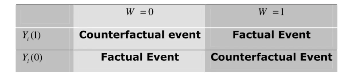
The factual event is the one that has been realised as the consequence of actual participation choice, while the counterfactual event is the one that would be realised if had the participation choice been different from the actual one (See Table 1.4 for the details)
1 Assignment mechanism can hardly be considered as unconfounded (unrelated to the potential outcomes) . See section
Table 1.4 The classification of potential outcomes respect to the participation status 0 = W W =1 ) 1 ( i
Y Counterfactual event Factual Event )
0 (
i
Y Factual Event Counterfactual Event
In our case, what prevents us to extract and quantify “the pure” program effect on the treated population is the fact that we cannot observe the counterfactual event of what would have happen to the participants had they not participated in one of the programs. The quantity of interest is the potential benefit for the individuals who participated into the programs and since the idea that lies behind is encouragement of such programs in future, if proved to be efficient.
One possible solution would be to construct a “similar” sample to the sample of participants in pre-program background characteristics. This was the solution of evaluation problem chosen in this research, especially because of the availability of a very rich background information on each individual, allowing to define a very good approximation for the counterfactual outcome – the one that the participants would have encountered in the case of non-participation.
In our case, the selected outcome variables (factual for both treated and non treated) assumed to be affected by treatment process are the following:
• A person is employed at the survey time (a dummy variable) • Person has been employed at least 6 months during 2000-2001 (a dummy variable)
• Person has been employed at least 12 months during 2000-2001 (a dummy variable)
• Number of months the person was receiving the unemployment benefit • Average monthly earnings at the survey time
1.7.2 The choice of the causal parameter of interest and the estimator
The framework of Rubin (1973) Heckman, Lalonde and Smith (1999) and Imbens(2004) was used to identify the “pure” effects of the policies, i.e. Average Treatment Effect on the Treated, defined as following:
) 1 | ) 0 ( ( ) 1 | ) 1 ( ( ) 1 | ) 0 ( ) 1 ( ( − = = = − = =E Y Y W E Y W E Y W ATET (1.1)
As mentioned previously, the main identification problem to be resolved is that E(Y(0)|W =1) is a counterfactual event defined in this context as what would have happened participants of ALMP, if they had not taken part into any program. The only quantity that can be derived is the empirical counterpart of the following:
) 0 | ) 0 ( ( ) 1 | ) 1 ( (Y W = −E Y W = E (1.2)
obtained as the difference between the mean outcome for the participants and non participants: ] ) 0 ( ) 1 ( [ 1 1 1 ^ 1 ^
∑
= − = N i i i Y Y Nτ
(1.3) where (0) ^ iY is the best approximation of counterfactual outcome for the treated.1
1.7.3 Selection bias
The problem of major concern when evaluating the effects in this context, i.e. in the context of non experimental design, is an eventual selection bias due to a correlation of individual program participation with
the outcomes of interest. In this case selection bias may arise from different “confounding factors”, one of which, certainly, is the individuals’ choice of ALMP to participate in (e.g., it is presumed that only the highly motivated workers take part into the programs; moreover, it is likely that more educated and more resourceful individuals could opt for Small Business Assistance program). Selection bias may also arise through screening operations of program operators, and in these cases we cannot absolutely talk about random assignment to different ALMP’s.
The measure in which selection bias can be reduced depends on a large scale on richness and quality of the baseline data collected. To be more precise, selection bias can be eliminated if, keeping all the relevant factors under control, the choice between participation and non participation among the individuals can be considered purely random. In Rodriguez Planas and Benus (2006) it is underlined that one of the strong points of the study was a very good data quality and collection of large number of individual baseline characteristics.
1.7.4 Propensity score matching
The practical problem of finding a comparison group, which would reflect, on average, similar characteristics to those of participation group, was resolved using propensity score matching, proposed by Rubin and Rosenbaum (1983).
Identification problem relies upon matching participants to non-participants similar in terms of observable characteristics X, and comparing outcome means net of compositional differences. Random selection conditional on the observables X implised that the following assumption hold:
• Unconfoundedness: For almost all x, the outcomes Yi(1),Yi(0) are independent of W , conditional on i Xi =xi, or:
x X W Y Yi(0), i(1))⊥ i | i = ( Condition (1)
• Overlap: For some c<0, and almost all x i c x X W c≤Pr( i =1| i = )≤1− 1 Condition (2) Under the unconfoundedness assumption (often stated in treatment evaluation literature as the Conditional Independence Assumption) it is as if the participation mechanism has been randomly assigned for each cell of covariate X, hence free of selection bias. However, if the number of X is very large (as in our case) cells of reasonable sample size become difficult to defined. This problem is the so-called curse of dimensionality.
This problem can be resolved using the propensity score e(x), the function that describes a relationship between the treatment dummy and the observable attributes of individuals. It is defined as following:
) | 1 Pr( ) (x W X x e = = = (1.4)
The propensity score therefore represents the conditional probability of participation given the pre-program characteristics X .
It follows that if the balancing property of background variables between participants and non participants is satisfied, observations with the same propensity score must have the same distribution of observable and unobservable characteristics, independently of participation status. This means that assignment to each of the groups is unconfounded, given the propensity score.2 The advantage of propensity score is a substantial reduction of the dimensionality problem of matching treated and control units on the basis of the multidimensional vector of X .
1
In fact, the common support restriction was imposed in psmatch2 algorithm for ATT
2
Thanks to propensity score, it was possible to detect a comparison group which was similar to participation group, along the line of the observed characteristics.1 The procedure passed through several steps:
i) A probit model was estimated, where a binary variable W =0,1 was regressed on a set of individual characteristics X . This was done for all pairs defined by either of the four ALMPs and the comparison group.
ii) Propensity score was estimated for all members of the participant and non participant groups.
For each member, a potential comparison group was assigned, based the propensity score, using the technique of kernel-based matching with a caliper of 1 percent. In this way a very few treated units were discarded, and each unit from the participation group were matched only with those comparison units who fall in a predefined radius. Therefore there was no poor matching. Note that the group of non-participants has been chosen only from those judets where the participants applied to the program, that is the participants were not compared to those non-participants registered at the EB in judets where the specific program was not facilitated.
1
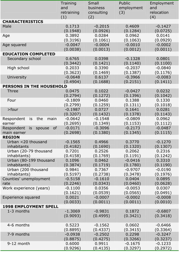
Table 1.5: Probit regression of the participation dummy on the observables Training and retraining (1) Small business consulting (2) Public employment (3) Employment and relocation (4) CHARACTERISTICS Male 0.1713 (0.1948) -0.2015 (0.0926) 0.4609 (0.1284) -0.1427 (0.0725) Age 0.3892 (0.3196) 0.0284 (0.1061) 0.0962 (0.1063) 0.0141 (0.0929) Age squared -0.0047 (0.0038) -0.0004 (0.0013) -0.0010 (0.0012) -0.0002 (0.0011) EDUCATION COMPLETED Secondary school 0.6765 (0.3442) 0.0398 (0.1421) -0.1328 (0.1140) 0.0801 (0.1100) High school 0.2033 (0.3623) 0.3390 (0.1469) -0.2037 (0.1387) -0.0840 (0.1176) University -0.0648 (0.4904) 0.6137 (0.1688) -0.3966 (0.2151) -0.0083 (0.1411) PERSONS IN THE HOUSEHOLD
Three 0.0475 (0.2794) 0.1022 (0.1272) -0.0427 (0.1396) 0.0232 (0.1042) Four -0.1809 (0.2799) 0.0460 (0.1259) 0.1388 (0.1311) 0.1330 (0.1018) >four -0.1987 (0.3207) 0.0727 (0.1432) 0.1641 (0.1378) 0.0281 (0.1143) Respondent is the main
earner -0.0642 (0.2695) -0.1548 (0.1349) -0.0809 (0.1153) 0.0962 (0.1112) Respondent is spouse of main earner -0.0171 (0.2698) -0.3096 (0.1380) -0.2173 (0.1345) -0.0487 (0.1115) REGION Urban <20 thousand inhabitants -0.1565 (0.4182) 0.4966 (0.1690) 0.3770 (0.1320) -0.1270 (0.1307) Urban (20-79 thousand inhabitants) 0.7201 (0.4158) 0.2526 (0.1769) 0.2062 (0.1191) 0.2316 (0.1242) Urban (80-199 thousand inhabitants) 0.1096 (0.3874) 0.0462 (0.1719) -0.0416 (0.1780) 0.3310 (0.1190) Urban (200 thousand inhabitants) 0.9841 (0.5197) 0.7367 (0.2738) -0.9707 (0.3478) -0.0190 (0.1976) Counties’ unemployment rate -0.5158 (0.2246) -0.1610 (0.0343) 0.0404 (0.0460) 0.0895 (0.0628) Work experience (years) -0.1100
(0.1621) 0.0356 (0.0539) -0.0053 (0.0565) 0.0307 (0.0491) Experience squared 0.0021 (0.0033) -0.0007 (0.0011) -0.0002 (0.0011) -0.0008 (0.0010) 1998 EMPLOYMENT SPELL 1-3 months -1.3069 (0.9093) -0.9831 (0.4995) 0.1872 (0.3421) -0.6807 (0.3418) 4-6 months 0.5223 (0.8895) -0.1562 (0.4337) 0.0602 (0.3415) -0.6466 (0.3364) 7-9 months -0.0938 (0.8875) -0.2502 (0.4275) 0.2298 (0.3266) -0.3247 (0.3237) 9-12 month 0.6000 (0.9296) 0.9911 (0.4135) -0.1675 (0.3297) -0.1233 (0.2972)
(Continuation of table 1.5) Training and retraining (1) Small business consulting (2) Public employment (3) Employment and relocation (4)
EMPLOYMENT AND SALARIES Average earnings per
month in 1998 (in thousand lei) (wage98)
-0.0016 (0.0004) -0.0000 (0.0001) -0.0003 (0.0002) -0.0001 (0.0001) 500-600 1.2480 (0.5833) -0.2457 (0.2943) -0.6796 (0.3086) -0.1813 (0.2096) 601-700 0.6409 (0.6015) -0.1330 (0.2491) -0.3222 (0.2664) -0.2447 (0.1841) 701-850 0.7412 (0.5189) -0.0327 (0.2146) -0.2518 (0.2322) -0.1748 (0.1699) 851-1,000 1.1921 (0.4614) -0.2962 (0.2074) -0.1687 (0.2432) -0.2043 (0.1626) 1,001-1,200 1.0384 (0.4632) -0.3793 (0.1985) 0.4523 (0.2317) -0.1763 (0.1623) 1,201-1,500 1.5699 (0.4754) -0.1055 (0.1973) -0.2128 (0.2754) -0.3851 (0.1724) 1,501-1,900 1.7622 (0.5584) -0.3607 (0.2263) -0.1731 (0.3575) -0.4094 (0.1939) 1,901-2,500 n.a. -0.3758 (0.2408) -0.8899 (0.4987) -0.9456 (0.2596) 1998 average unemployment spell (months) 0.6457 (0.1682) 0.3975 (0.0973) 0.2787 (0.0789) 0.5042 (0.0674) Avg. unemployment spell
squared -0.0646 (0.0149) -0.0289 (0.0092) -0.0181 (0.0070) -0.0387 (0.0071) 1998 unemployed at least 9 months 2.9805 (1.0990) 0.6637 (0.7353) 0.0427 (0.5104) 0.2608 (0.5406) TRAINING EXPERIENCE
Received training during 1998 -0.0509 (1.0856) 0.5994 (0.5027) -0.5666 (0.5482) -0.2614 (0.4207) 1998 average training length (months) 0.5509 (0.5871) -0.0084 (0.2405) 0.2683 (0.2746) 0.1144 (0.1907)
1.8 WHICH VARIABLES HAVE MOST EFFECT ON PARTICIPATION PROCESS?
It can be seen in Table 1.5 that when regressing the program participation dummy on different baseline characteristics it results that variables such as age, gender, family composition, level of education, previous work experience, and pre-program unemployment history are important
factors in determining whether an individual will participate in any program, as well as in which of the programs.
1.9 RESULTS
The effects, defined as a difference in mean outcomes between participants and comparison group, conditional on propensity score, can be found in the Table 1.6.
Table 1.6 Estimated Average Treatment Effects On the Treated for each ALMP Training and Retraining (1) Small Business Assistance (2) Public Employment (3) Employment and Relocation Services (4) OUTCOMES Current experience Employed 12.47 (9.18) 6.14 (3.34) 0.61 (3.15) 8.45 (2.75) Average monthly earnings (in
thousand lei) 65.67 (62.91) 37.58 (23.58) 3.10 (17.20) 56.86 (24.87) During the period 2000-2001
Employed for at least 6 months 2.53 (8.79) 8.38 (3.22) -7.36 (3.59) 6.22 (2.55) Employed for at least 12 months 8.06
(9.68) 7.97 (3.74) -8.45 (3.58) 7.65 (2.94) Average monthly earnings (in
thousand lei) 164.81 (69.82) 43.08 (25.13) -6.65 (20.08) 87.32 (19.37) Months unemployed -1.66 (1.95) -1.82 (0.65) 1.95 (0.67) -1.90 (0.59) Months receiving UB payments -1.01
(0.37) -0.75 (0.37) 0.21 (0.39) -0.74 (0.23) Sample size1 768 1,326 1,829 1,775
The estimates reflect the following pattern:
• Training and Retraining, Small Business Assistance and Employment and Relocation had a positive effect on probability of being employed in the period following the program.
• ER was successful in improving participants’ economic outcomes compared to non-participants in all dimensions.
• Small Business Assistance and Employment and Relocation have a positive effect on future salaries.
• Public Works program reduced the “unemployment spell”, but increased the likelihood of being currently unemployed.
For even better understanding of participation process, there are four groups of the variables that would be convenient to be observed and included in the propensity score:
• Pre-displacement job characteristics (such as earnings, occupation, job position, employer characteristics...);
• Variables concerning motivation, ability, social contacts... • Individual discount rates;
• The influence of the operators from Employment Bureaus and their eventual tendency to assign different individuals into different programs, and not randomly.
However, at the survey time they were not available, and further research would be needed to highlight their influence on the results.
Particularly useful information could be drawn from the study by observing differences in program impacts among different individuals.1
1
Chapter 2
Bootstrap methodology: Does it Always Work?
2.1 INTRODUCTION
Bootstrap methodology became a very popular tool when conducting inference, particularly in the last decade when executing laborious calculations on adequate software became less time and cost consuming.
For the discussion of the basics of the bootstrap idea, in what follows I will build upon Davison and Hinkley (1997) to summarise the methodology as well as the properties that are relevant to the problem I deal with in this dissertation.
The chapter starts with a brief introduction to the basic relevant theory about the bootstrap such as the origins and basic ideas behind the bootstrap, it points out the main types of bootstrap which can be found in the literature, in particular explaining simple non-parametric bootstrap - the one used in the previous chapter to draw inference on the effects of the program. Some practical questions are addressed, such as the number of replications requested for different types of parameters which are to be inferred, with possible errors that could be encountered.
The reader already familiar with the basic notions of bootstrap may want to skip sections 2.1-2.5 and go directly to section 2.6, dedicated to bootstrap
failure for matching estimators. The topic is strongly related to the article “On the failure of Bootstrap for Matching Estimators” by Abadie and Imbens (2004) about the failure of bootstrap method when evaluating the average treatment effects on the treated with nearest neighbour matching estimator.
The chapter ends with an illustration of different estimates produced by bootstrap estimator for standard errors of the ATT and the Abadie-Imbens estimator, introduced in the above mentioned paper.
2.2 BOOTSTRAP METHODOLOGY
Formalizing uncertainty is a key issue of any statistical analysis. Concretely, this means obtaining reliable measures of data variability, such as standard errors, confidence intervals etc. Uncertainty can be overcome by assuming a probability model for the available data; however this is rarely an easy task: simple and straightforward situations, where the data generating process is known, are quite a rarity especially in the context of socio-economic research.
The idea that stands behind the bootstrap is re-sampling from the original sample (directly or by a fitted model), in order to create copies of datasets, hence we do not have to define an underlying generative process. Using these generated datasets, inference on the quantities of interest (mean, standard errors, confidence intervals etc) can be drawn in computer-intensive and, only apparently, simple and straightforward way. Hence, the theoretical calculation is replaced by simulation.
The first article written on bootstrap methods was published by Efron (1979). The ideas of re-sampling methods were brought up even earlier; however Efron’s article was important because it gave a general framework to simulation-based statistical analysis. The popularity of bootstrap increased along with the improvement in computer performance over the past two decades, because simulated (bootstrap) distributions replaced those obtained from asymptotic theory.
Bootstrap is particularly useful when the analyst has to deal with the sample where basic asymptotic assumptions are not valid, such as when the sample size is small or when data distribution is not normal. Furthermore, bootstrap is a fairly easy tool in resolving complex inference when there is no reliable theoretic background of the problem; there is no need for making untestable assumptions on the underlying data generating process.
In conclusion, if the sample is a good approximation of the population, the belief is that bootstrap method provides a fairly good approximation of the sampling distribution of the estimator used to infer the parameter of interest.
2.3 CAN WE TALK ABOUT ONE TYPE OF BOOTSTRAP?
It would be quite misleading to talk about bootstrap generally, because there are many types of bootstrap depending on the type of data available. It can be restricted or unrestricted, residual, pairs, wild, moving-block, block of blocks etc.
Bootstrap methods can be done in two different frameworks – parametrically and non-parametrically.
When there is an assumption about the mathematic model underlying the distribution of Y – then we are talking about parametric models, where the economic theory suggests an underlying probability model for the data and the parameter of interest
τ
is a known function of some known constants or parameters.When it is only assumed that variables are independent and identically distributed – we are dealing with the non-parametric model. The empirical distribution of this model assumes equal probabilities
n 1
for each value Y from i
the original sample.
However, bootstrap should be applied only in situation where it is not possible to make assumptions about the distribution generating data, otherwise non-parametric procedures produce less efficient estimators (greater variance), wider confidence intervals and higher risk when compared to a parametric procedure.
2.3.1 The non parametric procedure
To fix our ideas, let us consider the situation where we measure the variable Y and we are interested in estimating the standard error
σ
related to its mean τ . Here we use the sample as an approximation of the population and we assume that the observations Y ,...,1 Yn are independent and identicallygenerated given observations. The bootstrap procedure in this case would be performed through the following steps:
• Step 1 : Resample with replacement in order to obtain * * 1,..., n
Y Y from
our original data, and finding the average
τ
b calculated on the pseudo-sample• Step 2. Repeat B (a moderate to large number of) times the same procedure in order to come up with the simulated distribution of
_
b
τ , that is:
τ
1 ,...,τ
B .• Step 3. Find a standard deviation of B estimates of means to obtain B
τ
σ . 1
2.4 ERRORS IN BOOTSTRAP
The choice of the bootstrap method for the estimation of quantities of interest, encounters the risk of committing two types of errors: statistical error and simulation error.
The statistical error in the parametric bootstrap is caused by the difference between empirical and assumed underlying distribution. Its magnitude depends upon the goodness of fit of the model chosen to approximate the data-generation process, the better it fits our empirical data, the smaller will be the statistical error in our estimates.
The simulation error is caused by the fact that estimated properties under sampling are used instead of exact properties. It may decrease by choosing a higher number of replications ( B ).
Another issue of interest when talking about bootstrap is number of “bootstrap samples” required in order to obtain reliable estimates.
The practical evidence suggests that in order to reduce the simulation error it is necessary to take B >100 to calculate bias and variance, while it is
advisable to consider even more than thousand replications if intended to estimate the quantiles for 95 percent confidence intervals. (See Davison 2006)
2.5 DOES BOOTSTRAP ALWAYS WORK?
2.5.1 Consistency of resampling methods
It is necessary to define an asymptotic framework (when sample size
∞ →
n ) to describe ideal conditions under which bootstrap works and provides results that can be trusted.
Suppose that we are dealing with a random sample Y ,...,1 Yn distributed
according to its empirical distribution function (EDF), and our quantity of interest is a certain function of our original data: τ = f(Yi). Furthermore, suppose we are interested in estimating the distribution function of the parameter
τ
, given the empirical distribution EDF (that is given the concrete realisation of the underlying process):{
}
^ ( ) Pr ( ) | n Y Y F τ = f y ≤τ EDFLet Ω be a suitable set of distributions that form a neighbourhood to the true distribution function
n
Y
F , and such that for n→∞ our ^
EDF falls into Ω with probability 1.
In order for the estimated distribution ( ) ^
τ
n
Y
F to approach the true distribution (τ)
n
Y
F as n→∞, it necessary that the following are satisfied (See Davison and Hinkley,1997):
1. For each distribution A belonging to some neighbourhood Ω in a suitable family of distributions, the distribution FA,n has to converge
weakly to FA,∞
3. The functional g:A→FA,∞ must be continuous 1
Under these conditions the re-sampling methods are consistent, that is for any
τ
and ε >0, Pr | ( ) , ( )| 0, ^ → − > ∞ τ ε τ Yn n EDF F
F for n→∞. Hence, we can
claim that the re-sampling method is valid. If any of these conditions fails, the bootstrap may fail too.
2.5.2 Asymptotic accuracy
The property of consistency is necessary but not sufficient for the ideal framework under which we draw valid interference using bootstrap. It is also desirable that the method chosen is the best possible one, in the sense that it reduces the unexplained variability the most.
Bootstrap methods fail when we are dealing with sistematically incomplete data. It also does not work neither with inter-dependent data, because it is against the principal assumption of re-sampling, where mutual independence of Y was imposed. Here it would be difficult to estimate a joint j
density of Y ,...1 Yn, given one realisation, and without independence assumption. However, for weakly dependent data, simple bootstrap methods work reasonably well. It is also essential that data is free of outliers.2
In order to derive a distribution of treatment effects on the treated, and be able to perform standard inference, a simple non-parametric bootstrap methodology was used in Rodrieguez Planas and Benus (2006). A better understanding of the theoretical background behind the bootstrap was essential in order to be aware of the possible risks concerning the validity of our inferential conclusions.
1 For more details see “Bootstrap Methods and their application”, Davison and Hinkley (1997), 2 For more details see “Bootstrap Methods and Their Application” Davison, Hinkley (1997)
2.6 FAILURE OF BOOTSTRAP METHODS
Abadie and Imbens (2004) brought into discussion the validity of bootstrap as a tool for performing the inference on the non-smooth estimators, such as matching estimators.
They argue that bootstrap inference for matching estimators has not been formally justified, and that there is reason to be concerned about their validity because of the non-smooth nature of some matching methods.
In particular, their work addresses the question of the validity of using bootstrap for nearest-neighbour matching estimators. Hence, they claim that in this case the actual variance differs significantly from the bootstrap variance.
2.6.1 Problem setting
In order to reach to a better understanding of the failure of bootstrap inference for certain types of matching estimators, in this section it was attempted to explain the concrete situation in which simulation-based inference fails to provide a valid confidence intervals.
Let us first introduce the nearest neighbour matching (NN) estimator. While kernel matching uses all the units from the non-participants group and associates them to the treated unit according to a different weight, NN involves finding for each treated individual that non-treated individual with the most similar covariates (or propensity score). 1
If it is possible that a single non-treated unit provides the closest match for more than one treated individual, hence the non-treated individual appears in the comparison group more than once. In the case of matching on discrete
1 The quality of match depends on the possibility to achieve that the selection bias across the treatment and comparison groups is minimised. However, it also discards potentially useful information by not considering any matches of slightly different propensity score. Relying too much on a reduced number of observations in the constructed comparison group can result in programme effects with larger standard errors.
observable X , it is also possible that one treated unit is matched to more than one non-treated unit (them having the same value of the covariate).
Hence, for each treated unit i, a set of the closest matches can be defined as follows:
{
}
( ) (1, 2,..., ) : j 0,| i j| min
J i = ∈j N W = X −X = (2.1)
The result of this type of matching process is the following treatment estimator:
∑
= − = 1 1 ^ 1 ^ ) 0 ( ) 1 ( 1 N i i i Y Y N τ (2.2) where∑
∈ = ) ( ^ ) ( # 1 ) 0 ( i J j j i Y i J Y .2.6.2 Bootstrap estimators vs Abadie-Imbens estimators
By analytical derivations confirmed by the simulation based findings Abadie and Imbens (2004) prove that the non-smooth nature of the matching estimator causes the invalidity of bootstrap based inference.
Building upon these findings, Abadie and Imbens (2004) proposed an alternative estimator of the variance of the nearest neighbour matching estimator, and provide a formal proof that the estimator is asymptotically correct. The rationale for what they did proceeds along the following lines. First, they reformulated the expression of matching estimator according to the discussion in what follows. The weighted number of times unit i is used as a match is K : i = = = =
∑
= N i i j J j J i K 1 i i 0 W if ) ( # 1 ) ( 1 1 W if 0 (2.3)∑
= − = N i i i i K Y W N1 1 ^ ) ( 1τ
.1 (2.4) Let 2 (X Wi, i)σ be the conditional variance of of Y given i W and i X . The variance i
estimator proposed by the authors of the articles is the normalized conditional variance: 1 2 2 2 1 1 1 ˆ ( ) ˆ ( , ) N AI i i i i i W K X W N σ σ = =
∑
− (2.5) where 2 1 AI AINσ =V . They demonstrate that the estimator is consistent: ^ 1( ( | , ) ) 0 p AI N V
τ
X W −V →On the other hand, the bootstrap variance estimator considered is the variance estimator that centres the bootstrap distribution of the parameter of interest
^
b
τ around the estimate t^ from the original sample: 2 ^ ^ ˆ ( ) ( b ) | , , Var
τ
=Eτ τ
− X W Y (2.6)The usual practice is calculation of these variances by performing bootstrap and obtaining B bootstrap samples; hence the empirical counterpart of the variance is: ^ ^ 2 2 1 1 ˆ ( ) B B b b B σ τ τ = =
∑
− (2.7) Fore some more details about the analytical expression of the true variance, and the proof that bootstrap variance may both over as well as underestimate the true variance see Appendix 2 for Chapter 2.
2.7 WHAT ABOUT THE BOOTSTRAP VARIANCE AND KERNEL MATCHING?
The authors (Abadie and Imbens (2004)) argue that in most standard settings, where not dealing with matching estimators, bootstrap is valid methodology and does not fail in providing confidence intervals.
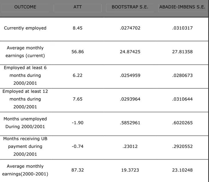
In order to investigate if the two different estimators of variance produce different confidence intervals for the ATT, we calculated Abadie-Imbens standard errors ˆσAI for each outcome variable. First it was done for
nearest-neighbour matching estimator (see table 2.1), in order to reproduce the set up to described in Abadie and Imbens (2004), where bootstrap failed. Second, it was done using our matching estimator (see Table 2.2).
In the first place, we observe that nearest neighbour matching estimator produces the ATT estimates different from the kernel-based one. Next, we can observe an interesting pattern when comparing the s.e. estimates. When using kernel matched data – our ˆσAI estimates are systematically higher than the ˆσB
estimates. In the nearest neighbour illustration we have exactly the opposite, and the bootstrapped standard errors seem to be systematically higher than the Abadie-Imbens ones.
In order to test the significance of these differences, as well as to attempt to answer the question which estimator works better in our case, Monte Carlo evidence is needed, and will be presented and discussed in the next chapter.
Table 2.1: Bootstrap vs AI standard errors (Nearest Neighbour Matching)
OUTCOME ATT BOOTSTRAP S.E. ABADIE-IMBENS
S.E. Currently employed 8.43 .0402767 .0380963 Average monthly earnings (current) 66.79 34.32143 33.61141 Employed at least 6 months during 2000/2001 3.75 .036321 .0350155 Employed at least 12 months during 2000/2001 7.76 .041704 .038385 Months unemployed During 2000/2001 -1.24 .8132401 .7433141 Months receiving UB payment during 2000/2001 -0.92 .3664738 .376705 Average monthly earnings(2000-2001) 91.17 28.68235 28.43399
Table 2.2: Bootstrap vs AI standard errors (Nearest Neighbour Matching)
OUTCOME ATT BOOTSTRAP S.E. ABADIE-IMBENS S.E.
Currently employed 8.45 .0274702 .0310317 Average monthly earnings (current) 56.86 24.87425 27.81358 Employed at least 6 months during 2000/2001 6.22 .0254959 .0280673 Employed at least 12 months during 2000/2001 7.65 .0293964 .0310644 Months unemployed During 2000/2001 -1.90 .5852961 .6020265 Months receiving UB payment during 2000/2001 -0.74 .23012 .2920552 Average monthly earnings(2000-2001) 87.32 19.3723 23.10248
Chapter 3
Monte Carlo Simulation
3.1 INTRODUCTION
In the previous chapter we have provided evidence of non-negligible differences that exist between the variance of the average treatment effect on participants as estimated via bootstrap vis-à-vis the variance estimated using the Abadie-Imbens estimator. Since we do not know the expression for the “true variance” of the kernel matching estimator to be exploited to draw causal inference on the effects of the program, on the basis of the evidence provided we cannot conclude which estimator of the variance performs better in terms of the distance from the “true variance”. This may be rather inconvenient in general, since we are not able to draw the most reliable inference on the parameter of interest, for example in terms of it’s significance or to calculate reliable confidence intervals.
In order to provide an answer to this question, in this chapter we will produce evidence from a Monte Carlo simulation that will allow us to shed more light on this problem, at least for the case of the data on ALMP’s in Romania.
This chapter therefore completely focuses on the simulation exercise. It illustrates, step by step, the logic and the procedure used to obtain the three different simulated distributions:
• Distribution of the Average Treatment Effect on the Treated;
• Distribution of the bootstrap standard error for the matching estimator;
• Distribution of the Abadie-Imbens estimator of the standard error of the matching estimator.
The remainder of this chapter is organised as follows. Section 3.2 highlights certain aspects of the sample we chose for the simulation; Section 3.3 describes the the logic behind the choice of data generating process as well as the methods used to derive the three distributions of interest; Section 3.4 briefly introduces the reader to some practical computational aspects and difficulties in performing our experiment, while the results of the simulation exercise are presented in the Section 3.5.
3
.2 THE CHOICE OF THE SAMPLEThroughout this chapter we will focus only on one program of main interest amongst those in the package offered by the ALMP’s in Romania, that is the program named Employment and Relocation services. Very pragmatically, our choice was driven by the sample size of the participants involved relative to that of the other three programs. Therefore, the sample size consists of 1775 individuals, out of which 747 participants and 1028 non participants.
The outcome variable selected is labelled as “currently employed” and it is a dummy variable which indicates if the individual were employed (Y =1) or unemployed (Y =0) at the survey time (Jan/Feb 2002). There is no particular criterion that underlies the choice of this specific outcome.
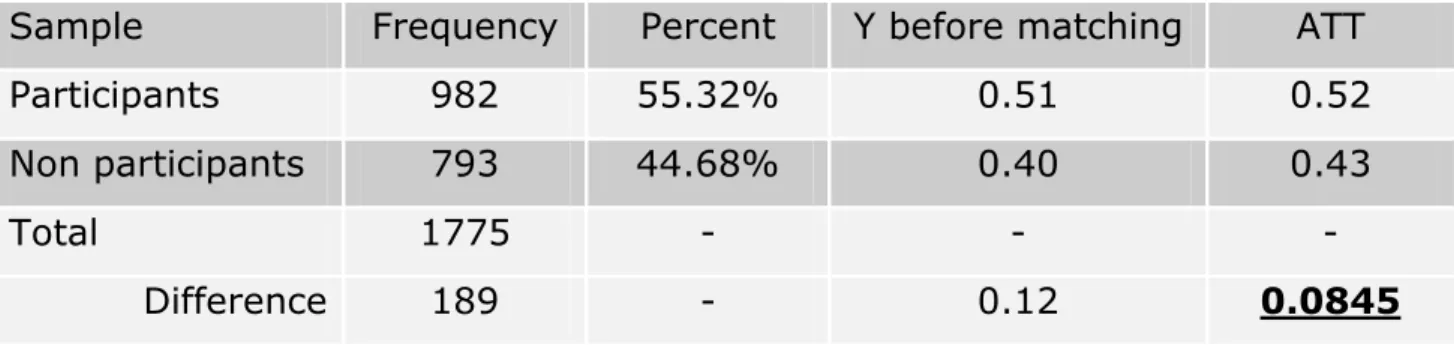
The summary of our sample, respect to the outcome variable is tabulated Table 3.1. In this table we present the proportion of individuals at work ad the survey time separately for the participants and non-participants, as well as the outcome difference before and after matching.
Table 3.1: The sample summary of the outcome respect to the participation status Sample Frequency Percent Y before matching ATT
Participants 982 55.32% 0.51 0.52
Non participants 793 44.68% 0.40 0.43
Total 1775 - - -
Difference 189 - 0.12 0.0845
3.3 GENERATING DISTRIBUTIONS
The parametric counterpart of the matching estimator adopted in the Chapter 1 is the ordinary least squares (OLS) estimator of β1 obtained from the following regression:
0 1 1 1 2 2 ... m m
Y =β β+ W +δ X +δ X + +δ X +ν (3.1) where:
• β1 - Average treatment effect on the treated
• δi - Effects of each specific covariate on the outcome
• m- Number of covariates X •
ο
is the residual termEquation (3.1) simply retrieves the causal parameter of interest by comparing the outcome mean for participants (W =1) and non-participants (W =0) net of compositional differences represented by X (hence controlling for all the available covariates). These variables are exactly those that guarantee the unconfoundedness condition stated in Section 1.7.4, which represents the key identifying restriction that we maintained throughout this thesis.
Note, however, that if the condition of unconfoundedness holds with respect to X , it has to be the case that it also holds conditionally upon the
propensity score e x( ). As we have discussed in Section 1.7.4, this represents the main result by Rosenbaum and Rubin (1983) that we exploited to obtain point estimates of the program effect.
The aim of this section is twofold. First, we show that estimates of the ATT obtained via matching provide an equivalent information to those for β1 obtained from equation (3.1) (see results in Table 3.3). Second, we show that the same result holds if instead of controlling for X in equation (3.1) we control for a polynomial in ( )e x of an adequate order, that is if we run the following regression:
( )
( )
2( )
30 1 1 2 3
Y =β β+ W+δe x +δ e x +δ e x +ζ (3.2) and obtaining the coefficients estimates listed in the Table 3.2.
Table 3.2: OLS regression summary relative to the equation 2
Root MSE = .49326
Adj R-squared= 0.0162
Coefficient Estimate Standard Error
p-value Confidence Interval at 95% constant 0.4198 0.0198 0.000 (0.3811 ; 0.4586) 1 β 0.0851 0.0269 0.002 (0.0323 ; 0.1378) 1 δ 0.0354 0.0263 0.177 (-0.0160 ; 0.0870) 2 δ 0.0056 0.0152 0.711 (-0.0242 ; 0.0354) 3 δ 0.0010 0.0093 0.286 (-0.0084 ; 0.0283)
Recall that the propensity score ( ( )e x ) for each individual has been retrieved using a probit regression of the binary response variable that indicates the participation (W ) on individuals’ background information variables. The results from this regression were reported in Table 1.4.
We found that if the order of the polynomial for ( )e x is three, OLS estimates obtained from the regression in (3.2) provide values of the β1
coefficient close to the effect estimate obtained via matching. Note that in our simulation we focused on a linear probability model rather than estimating a binary model for the equation in (3.2), thus ignoring the binary nature of the outcome variable.
Table 3.3: Parameters of interest across the different types of matching
ESTIMATION METHOD
ATTStandard Errors
Confidence intervals
Non parametric matching with bootstrap
0.0845 0.0275 (0.0319 ; 0.139)
OLS regression based on all the covariates
0.0835 0.0226 (0.039 ; 0.128)
OLS regression based on propensity score
0.0850 0.0269 (0.0323 ; 0.1378)
Our root mean square error term
ε
is a higher than it would be if we used all the covariates Xi (0.49 respect to 0.42), and the adjusted R2indicates the better data fit in the full regression (see Appendix 1 for Chapter 3 for the full regression results). However, as we can see from Table 3.3, in terms of ATT estimate the results are coherent and that there is no important information loss if we reduce the covariates in the full regression only to propensity score terms: while the non parametric ATT estimate amounts 0.08451 percent, regression based estimates for β1 are quite close.
3.3.1 Data generating process
In order to be able to generate the distribution of matching estimator for the program effect we first assume that the outcome observations Y were generated by the equation containing the propensity score:
( )
( )
( )
2 3
0 1 1 2 3
ˆ ˆ ˆ ˆ ˆ