The Natural Connectivity of Autonomous Systems
Steve BattleDept. Computer Science and Creative Technologies University of the West of England, Bristol
Abstract The principle of biological autonomy, introduced by Francisco J. Varela, addresses the dilemma of Cartesian mind-body dualism by re-casting mind and body, or subject and object, observer and observed, not as irreconcilable categories, but as complementary perspectives on the same biological phenomena. Indeed, this distinction between self and non-self may be seen as a necessary pre-condition for autonomy. An autonomous system is self-governing in that it is concerned with preserving its unique character, or unity. Furthermore, an autonomous system is operationally closed in that it forms a self-referential network without reference to an external world. This paper develops these ideas in relation to thinking about embodied, enactive robotics. As well as being constructed artefacts, what is it to look at robots as truly autonomous agents? In this context we begin to explore the concept of operational closure analytically. We utilise natural connectivity as a quantitative measure of the cyclicity of these operationally closed internal processes. In doing so we discover that increased natural connectivity of an autonomous system confers a greater behavioural robustness when it is coupled with the external world.
Keywords: autonomy, operational closure, enactive, embodied Received 07/03/2020; accepted 05/04/2020.
0. Introduction
Varela’s enactivism (Varela et al. 1991) is an approach to understanding how robots can operate autonomously in the human environment. The approach is rooted in the existentialist philosophy of Martin Heidegger (Heidegger 1962) and his ideas of the nature of human existence as being thrown into the world. These ideas were taken further by Maurice Merleau-Ponty (Merleau-Ponty 1962) who described the self as a unification of mind and body, with all the physical needs that entails. Where a disembodied computer has no real needs, a mobile robot has very real power requirements to satisfy; an autonomous robot is thrown into this world just as we are. On a practical level a mobile robot must be able to find a power source and charge its batteries to remain viable. While this may not count as a lived experience, for robots are not alive, can we speak in terms of a robot being an autonomous agent?
Varela’s Principles of Biological Autonomy (Varela 1979) emerged alongside Maturana and Varela’s Autopoiesis (Maturana, Varela 1980). Autopoiesis addresses the question of what it means to be alive and is concerned primarily with the physical self-production of living beings as characterized by the dynamic process of cellular regeneration. Living beings are autonomous by virtue of their autopoietic nature; an organism faces the world on its own terms, driven by the need to find sustenance. It would be a mistake to apply autopoiesis to our current technologies as conventional computers and robotics clearly do not have this regenerative capability. While autopoiesis implies autonomy, the reverse is not the case. Varela’s (Varela 1979) definition of autonomy focuses instead on the unity brought about by self-organization. This refers to the self-organization of processes within the organism that ultimately produce observable visible behaviours. By behaviour we mean goal-oriented activity produced by an organism or agent, rather than the motion of a passive object. This choice is influenced by Merleau-Ponty in The
Structure of Behaviour (Merleau-Ponty 1942: 36), «the motor devices appear as the means
of re-establishing an equilibrium, the condition s of which are given in the sensory sector of the nervous system». These behaviours constitute a closed homeostatic loop with the goal of ensuring continued survival. This latter theory is far more pertinent to AI and autonomous robotics; whilst not alive, an autonomous robot must protect its own existence; its identity, as realised by a complex set of behaviours.
1. Robot and environment
We are interested in autonomous behaviours that enable robots to function semi-independently of humans. Organisms and robots are structurally coupled with their environments through sensorimotor activity; this is their interface with the environment. One advantage of working with robots is that it is straightforward to record their behaviour, capturing not just movement but also incoming sensor data. The working example used throughout this paper is W. Grey Walter's ELSIE robot (Walter 1953). The name is an acronym for Electro-mechanical Light-Sensing robot with Internal and External stability. It has a functional simplicity that lends itself well to experimentation, and yet it is also an autonomous robot in that its behaviour exhibits a long term viability as it is also able to periodically recharge its batteries, much like a modern robotic vacuum cleaner. These Machina Speculatrix, as Walter called his family of robots, were not digital computers, but were analogue electronic creatures. It wasn’t simply that stored-program digital computers didn’t physically exist until 1948, the same year ELSIE was built, but according to Walter, no «variety of programming endow a machine with the autonomous qualities of a true mimicry of life». Whatever the truth of this, we can explore the behaviour of these creatures by simulating them in software.
Fig 1.
ELSIE simulation: the scanning turret (direction in green) contains a single photo-cell, and the shell senses obstacles through mechanical contact. As the characteristic epicyclic path of the robot is traced
out, it can be seen that this path is an orbit around the light-source at the centre of the figure. In order to understand ELSIE’s behaviour, a software simulation was constructed. This is not a deep simulation of the electronics, but is a rule-based behavioural model coupled with a two-dimensional kinematic simulation of the robot hardware. The simulated environment is populated by random obstacles and a single source of light and power. A screen-capture of the ELSIE simulation can be seen in Fig 1. The output includes a trace of the robot’s path displaying the characteristic epicyclic trajectory. ELSIE has separate drive and steering motors both ingeniously connected to the front wheel. These run at different speeds according to the current state. The front drive wheel is fixed to a rotating turret, topped by a photocell aligned with the forward direction of the drive wheel. The photocell is directional and this direction is indicated in the simulation by a green line emanating from the turret. As this scanning photo-cell sweeps across the light source, its circuitry is stimulated by the increasing light level to increase the speed of the drive motors, while simultaneously reducing the scanning speed. This behaviour gradually brings the robot closer to the light where the battery charger resides.
On encountering an obstacle, the movement of the outer shell pressing against it activates a ‘trembler’ switch. When this happens the robot enters an oscillatory state that flips rapidly between pushing and turning, «The steering-scanning motor is alternately on full- and half-power and the driving motor at the same time on half- and full-power» (ibid.). This enables ELSIE to wriggle free of the offending obstacle both in reality and in simulation, as shown in Fig. 2.
Fig. 2
ELSIE simulation: obstacle detection is simulated by detecting the intersection of the robot's bounding box with that of an obstacle; the square box. As in the real system, the contact signal persists for a short
period after breaking contact.
Even though this behaviour is continuous and analogue, it may be classified symbolically. The classifications used here are the set of symbols (E, P, N, O, R) and this classification captures both sensor data and motor activity. This combination of sensor and motor activity is deliberate. Merleau-Ponty teaches us that «the sensorium and motorium function as parts of a single organ» (Merleau-Ponty 1942: 36). If it were like anything to be a robot, then this combined sensorimotor activity might be said to constitute its subjective phenomenological experience.
ELSIE’s usual mode of behaviour is to explore (E) the environment driving forward slowly with a rapidly scanning turret searching for the light source. As it encounters obstacles (O), ELSIE wriggles free of them with the oscillatory motion described above. ELSIE is attracted to light from afar – positive phototaxis (P), stopping the scanning motor to keep the light source in view for as long as possible. As it approaches a light source on a full battery it is repelled from the bright light – negative phototaxis (N), turning slowly away from it. Only when the battery is low is its repulsion to bright light overcome, allowing it to approach the light source and recharge (R), at which point both motors are disconnected until she is fully recharged. These behaviours are summarised in Table 1. This simulation is used to generate data for both training and testing.
behaviour pattern collision light level scan/drive
E - Exploration no low fast/slow
P - Positive phototropism no medium stop/fast
N - Negative phototropism no high slow/fast
O - Obstacle avoidance yes ANY 1Hz oscillation
R - Recharge no ANY stop/stop
Table 1.
From an enactive perspective, this is sensorimotor data only from an external observer’s perspective (Varela et al. 1991). By definition, an enactive system has no direct input/output, but of course a robot does have sensors and actuators. While there is no place for external data within an operationally closed autonomous system, external
perturbations may push an autonomous system from one state into another. The
behaviour patterns in Table 1 form a so-called domain of interactions; the domain of all perturbations/actions the system may undergo without loss of autonomy.
The behavioural data define a simple language formed of sequences of symbols produced by the robot embedded within its environment. These symbols are arranged in a string where the left-to-right order represents observable behaviour in the world as time passes. We record only changes in state, so no pairs of neighbouring symbols are alike. To emphasise viable behaviours, the simulation includes a virtual battery that rapidly runs down as ELSIE explores the environment. As the battery runs down ELSIE must seek to recharge or else it will cease to function. Table 2 shows a small sample of this data. For simple autonomous systems we assume that this is a Chomsky Type 3 regular grammar which can be accepted by a finite state automaton. This is sufficient to explore a wide range of viable autonomous behaviours.
EPEPEPNPEPNPE… EPEPEPNPEPNPE…
EPEOEPONOEOPEPEPE… EPEPOPNPEPRNPE…
⋮
Table 2. Samples of observed behaviour
2. Autonomous systems
While the analogue behaviour of robots like ELSIE can be described as dynamical systems, Varela sought alternative approaches that could be used to understand the cyclic and closed nature of autonomous systems. In Principles of Biological Autonomy (1979) Varela explores the ‘logic of distinctions’ expounded by G. Spencer-Brown (1969) using this to discover autonomous recurrent states. In this paper, Finite State Machines serve a similar role and may be more familiar to a modern audience. This enables us to analyse cyclic behaviours in terms stable dynamics known as eigenbehaviours (von Foerster 2003). This eigenbehaviour is the signature of the autonomous system, constituting its very identity.
Each node of a state-machine represents a distinct, separate state, which is a simple and effective technique for primitive robots, but with increased complexity the method would quickly get out of hand due to combinatorial explosion. As an autonomous system a state-machine satisfies the requirement for organizational closure. With no input/output to consider, the transitions of the state-machine are unlabelled and simply connect one state to another forming a closed graph. It is state-driven and finite, and is therefore capable of generating cyclic behaviour. For this analysis we are interested in the fundamental ‘loopiness’ of the autonomous process.
The nature and number of states is not to be identified with the externally observable classes of behaviour described in the section above. The states are hidden, in that the states that the autonomous system passes through are not directly observable. State is hidden in the same sense that it is hidden in a Hidden Markov Model, but for the analysis of the autonomous system used here we do not require the probabilistic parameters (transition and output probabilities) of the HMM.
A state-machine in the form of a directed graph can be represented as a square adjacency matrix, where a one at the intersection of a particular row and column represents a possible transition from the current state (row) to the next state (column). The coupling between the autonomous system and its environment, or at least a symbolic description of it, is provided by another matrix that relates the hidden states of the autonomous system to the behavioural sensorimotor symbols. This is an incidence matrix relating hidden states to output symbols. The sensorimotor symbol can be described as a function of the current state, permitting multiple states to emit the same symbol but without the additional variability that HMMs allow for with a vector of output probabilities associated with each state.
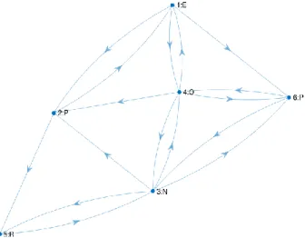
Fig. 3
A 6-state machine produced by generating a Hidden Markov Model and discarding the transition probabilities has more edges than necessary to accept the sample behaviours. The graph shows each node
number and emission symbol.
The adjacency matrix can be constructed using the tools for training Hidden Markov Models. Given one or more symbol sequences (emissions) it is possible to estimate the transition probabilities for a hidden Markov model using the Baum-Welch algorithm (Baum et al. 1970), a hill-climbing search that will converge to a local maximum from an initial randomised HMM (using the MATLAB function hmmtrain). The emission matrix can be initialised to a random incidence matrix with a functional mapping from states to emission symbols (a single one in each row). The transition probabilities it returns may be converted into possibilities by mapping all positive probabilities > 0, to 1. However, it seems wasteful to calculate the full transition matrix and then discard the probabilities in this way. There is a further issue with this approach. In addition to this wastage, graphs generated in this way have more edges than necessary to capture the behaviours in the training set, see Fig. 3 for an example. An alternative edge-removal algorithm shown in Table 3 is able to generate the adjacency matrix directly.
edge_removal(trials, m: side of square matrix) score = 0
for i = 1:trials
% adjacency matrix a, emission matrix e a = ones matrix - leading diagonal of size m
e = random emission matrix (single 1 on each row)
x = random permutation of indices in a (excluding leading diagonal) for j = 1:length(x)
a[x[j]] = 0
if a is no longer a connected graph break outer loop
if not all observations can be generated by a,e a[x[j]] = 1 % reverse edge removal
% natural connectivity n = log(trace(expm(a))/m)
if a is connected graph and n > score adjacency = a
emission = e score = n
return adjacency, emission, score
Table 3
Edge-removal algorithm finds the smallest viable graph with the maximum natural connectivity. The inner loop starts with a fully connected graph and removes edges one-by-one at random leaving the
smallest graph that remains viable.
from/to 1 2 3 4 5 6 1 0 1 0 1 0 1 2 1 0 0 0 1 0 3 0 1 0 1 1 1 4 1 1 1 0 0 1 5 0 0 1 0 0 0 6 0 0 1 1 0 0 Fig. 4
Square adjacency matrix corresponding to the graph in Fig. 7, showing transitions from states
in rows 1-6 to states in cols 1-6. This represents the autonomous system
independent of input/output. E P N O R 1 1 0 0 0 0 2 0 1 0 0 0 3 0 0 1 0 0 4 0 0 0 1 0 5 0 0 0 0 1 6 0 1 0 0 0 Fig. 5
Incidence Matrix representing the functional ‘emission matrix’ for the graph in Fig. 7, mapping states 1-6 to the sensorimotor
The intuition here is that we can begin with a matrix of ones, and then knock-out the edges (flipping matrix elements from 1 to 0) at random, subject to a check that this hasn’t eliminated the potential for some observed behaviour; the graph must remain viable. In fact, as the graph is not reflexive the main diagonal can be knocked out from the start. At each step the training set is consulted to ensure that all observed behaviours remain a possibility. If the adjacency matrix fails the test, then the change is reversed. This process continues until no more elements can be changed without failing the test. As before, the emission matrix is generated randomly and is held constant throughout. The square adjacency matrix in
Fig. 4 represents the edges in the graph representing the autonomous system independent of any input/output, while the matrix in
Fig. 5 represents the sensorimotor coupling between the autonomous system and the environment. This is graphically illustrated in the leaner graph of Fig. 6.
Fig. 6
This 6-state machine generated by edge-removal captures nodes emitting identical symbols, ‘P’, but in different contexts after reaching states 2 or 6.
To test that a state-machine can potentially generate a behaviour, it must be treated as a non-deterministic finite-state-machine. At any given time it can be in multiple states; all the states that potentially may have been reached. In the initial configuration, any and all of the states are a possibility. As each behavioural symbol is consumed, some states are knocked out that cannot make that transition, and others are added as all valid transitions are followed. If at any point the state configuration is empty, then the state-machine fails the test.
For a given graph size, the edge-removal algorithm produces many candidate graphs each with a different random emission matrix as a starting point. How might we select among them? A measure is required that enables us to maximise the potential for cyclic behaviour.
With an autonomous system captured in this form it is possible to carry out an analysis based on the number of walks that can be made from any node back to itself. From a
range of graph centrality measures, subgraph centrality (Estrada, Rodríguez-Velázquez 2005) emphasises the cyclic, oscillatory patterns of behaviour that are the hallmark of autonomy.
Subgraph centrality is based on the number of closed walks from a node back to itself, a closed walk being a succession of edges starting and ending at the same node. The number of walks of length k between any two nodes in the graph can be computed by raising the adjacency matrix to the power k, or Ak. Subgraph centrality (ibid.) is defined as the weighted sum of the closed walks of length k starting and finishing at a given node. The subgraph centrality, SC, of A for node i is defined in equation 1 below. To achieve convergence a weighting of 1/k! is applied, with the effect that short walks have more influence on the centrality of the node than long walks.
The subgraph centrality, defined in Equation 1, is equivalent to the diagonal entry of the matrix exponential of the adjacency matrix, eA (Estrada, Higham, 2008).
Equation 1. Subgraph centrality
The Estrada index (Peña et al. 2007), defined in Equation 2 below, is the sum of the elements of the subgraph-centrality. This is equivalent to the trace (sum of the diagonal) of the adjacency matrix exponential.
Equation 2. Estrada index
The natural connectivity of an autonomous system can be understood as the degree of redundancy in the number of closed walks from any node back to itself. If one walk should be unavailable, then another may be taken in its place. The Estrada index grows quickly for large numbers of nodes, so the natural logarithm of the averaged Estrada index may be used as a measure of the natural connectivity of a graph (Wu et al. 2009), defined in Equation 3 below, where n is the number of nodes (hidden states).
Equation 3. Natural connectivity
The natural connectivity of the graph has the nice feature that it changes monotonically with the removal (or addition) of edges (Wu et al. 2009). As the graphs produced by edge-removal have fewer edges than those derived from the Hidden Markov Model, they have correspondingly lower indices.
Fig. 7
A 9-state machine generated by edge-removal with minimal natural connectivity (min-connectivity). During the edge-removal search, the natural connectivity index falls monotonically with each edge removal. As this index is independent of the emission matrix and depends only on the adjacency matrix, it allows us to compare alternative solutions. It is worth re-iterating that this gives us a measure of the robustness of an autonomous system,
without regard to its behaviour. The focus is entirely on a system's ability to maintain its
organisation seen as a recurring process. Non-connected graphs are eliminated at this stage as the Estrada index depends only on the Estrada indices of its connected nodes (Du 2013). Of all the remaining minimal graphs, it allows us to discover the most robust solution with maximal natural connectivity. The 6-state solution of Fig. 6 was found within 1000 independent trials.
The interesting thing about the graphs of both Fig. 3 and Fig. 6 is that in both cases the search appears to have ‘discovered’ the underlying ‘EPNPE’ cycle that occurs while the robot, ELSIE, is orbiting around the light source. As the turret rotates it transitions from a low light-level (E) facing away from the light, through an intermediate spike of medium level light (P), to bright light (N), and then back again (P) as it veers away from the light. These state-sequences are primarily a feature of its electro-mechanical construction, rather than its electronic circuitry. As two of the hidden states map to ‘P’, more of the different contexts of these two ‘P’ emitting states is captured in the graph.
Fig. 8
A 9-state machine generated by edge-removal with maximal natural connectivity (max-connectivity). What does it mean in practice to maximise natural connectivity? The edge-removal algorithm destroys a huge amount of robustness and potential behaviour, so we’re working at the fringes with resource limited systems having a fixed set of states and only a minimal number of state-transitions. What is the virtue of maximising natural connectivity – retaining whatever potential the system has – rather than further minimisation of natural connectivity at this stage? An example of a graph with minimal natural connectivity ( =0.3836) is shown in Fig. 7; call this the minimal graph. This is a graph with 9 nodes mapping onto the same set of 5 behavioural patterns, so we see more nodes mapped to the same output. Contrast this with the 9-node graph with maximal natural connectivity ( = 0.9059) in Fig. 8. There’s no discernible difference between the in or degree of either graph. The minimal graph has mean in and out-degrees of 2.11 (they are equivalent in this respect), while the maximal graph has mean in and out-degrees of 2.33.
The clearest difference between these graphs is in the number of short-cycles evident in their structure. This should come as no surprise as this is precisely what the Estrada index measures, and indeed it gives more weight to these shorter cycles. As we saw above, the number of walks of length k between any two nodes in the graph can be computed by raising the adjacency matrix to the power k, or Ak. The trace of A2 divided by 2 is the number of directed digons (2-sided directed polygons in the graph), while the trace of A3 divided by 3, is the number of directed triangles. The division is necessary as we can walk the path starting at any of its vertices. The tr(A2 )/2 = 3 digons in Fig. 7, and tr(A2 )/2 = 6 digons in Fig. 8, may easily be counted. The pattern doesn’t straightforwardly extend to squares as digons also produce 4-cycles. However, the Estrada index is not concerned with whether such 4-cycles are generated by squares or combinations of digons. Table 4 informally summarises short 2, 3, 4, 5 & 6-cycles found in these examples of minimally and maximally connected directed graphs. It can be seen
that the tendency in maximally connected graphs over minimally connected graphs is towards these cycles. Both graphs are sufficient to produce the observed behaviours in the training set, so it is plausible that the reduced performance of the minimal graph is due to over-fitting to the training data.
graph tr( A2 ) tr( A3 ) tr( A4 ) tr( A5 ) tr( A6 )
min-connectivity 6 0 22 20 72
max-connectivity 12 15 64 140 435
Table 4
n-cycles in minimally and maximally connected directed graphs.
3. Experimental results
To validate the autonomous system against the symbolic data of recorded test behaviours, we may evaluate the state-machines produced by the edge-removal algorithm against the test-set of behaviours. As in the algorithm itself, we test for the
possibility that the test sequences could be produced by the state-machine. The
hypothesis is that there is a correlation between the natural connectivity of an autonomous system, and the corresponding success rate when evaluated against the test set of behaviours. It isn’t immediately obvious that this should be the case, as natural connectivity is a function of the graph topology of the autonomous system alone. We are really asking if the qualitative features of the graph favoured by natural connectivity support generalisation from the training data to the test data.
The output of the edge-removal algorithm is a set of connected graphs that are consistent with the training data. Each graph is minimally sufficient to generate the observed data such that the removal of any one edge would result in a failure to match at least one of the observations. However, while the number of nodes is constant, the graphs produced don’t always have the same number of edges. Intuitively, the more edges there are in a graph, the more likely it is to be effective. Fig. 9 shows the distribution of edges for an 8-node graph produced by edge-removal, which can be seen to be normally distributed. These are normally distributed as indicated by the R-Square statistic (0.9988), which being close to 1 indicates that the fitted Gaussian model accounts for over 99% of the variation.
Fig. 9
Bar-chart of the number of edges produced by 1000 iterations of the edge-removal algorithm for an 8-node graph. 86% of the graphs were eliminated as non-connected. The count of the remaining graphs are
plotted against the number of edges.
A confounding factor is that the probability of passing a test is correlated with the number of remaining edges. In Fig. 10 we see a clear linear correlation between the number of edges and the probability of passing a test. With a p-value < 0.001 we reject the null hypothesis of no correlation in favour of the alternative hypothesis of a linear correlation. Clearly, the more edges a graph has, all the better for matching a novel behaviour in the test set. The number of edges is factored into natural connectivity, as we saw that removing an edge results in a monotonic decrease in natural connectivity. However, we must show that any effect is not simply down to the number of edges, but is a result of the cyclicity of the graph.
Fig. 10
Plot of the number of edges produced by 10K iterations of the edge-removal algorithm for an 8-node graph. 85% of the graphs were eliminated as non-connected. The plot shows the average number of tests
passed for each given edge count.
To eliminate the effect of the number of edges on the probability of passing a test, we must hold the number of edges constant. We select the median value (in the case of an 8-node graph, the median is 17) to maximise the number of samples. In Fig. 11 we see that even after eliminating the effect of the number of edges, that there is a strong correlation between the natural connectivity and the probability of passing a test. The binomial number of tests passed or failed over 100K trials are summed across 50 bins, each representing a range of values of the natural connectivity. The averaged natural connectivity of the graphs is plotted against the probability of passing a test. The y axis is normalised to the range [0,1] and a logistic model is fitted. With a p-value = 0.0173 the fit is significant at the 5% level. We reject the null hypothesis of no correlation in favour of the alternative hypothesis of a generalised linear (logistic) correlation. If natural connectivity has no bearing on this then we would expect the passes and failures to be evenly distributed. This effect must be attributable to the cyclicity of the graph as described by operational closure.
Fig. 11
The effect of the number of edges on the probability of passing a test can be eliminated by holding the number of edges constant. In this case, we explore an 8-node graph and select only solutions containing
the median number of edges (17).
We conclude that graphs with high natural connectivity (cyclicity) confer a built-in redundancy, or robustness that lends itself to generalisation from the training data to the test data.
4. Conclusion
Starting with Varela’s definition of an autonomous system as an operationally closed system, we utilise state-machines to represent processes in which stable eigenbehaviours exist and can be analysed using a graph centrality measure known as natural connectivity. This is a good measure of the kind of cyclic behaviour we associate with autonomous systems. An edge-removal algorithm allows us to generate state-machines from robot simulation data which maximise natural connectivity for any given number of nodes and edges. It is important to reiterate that the evaluation of natural connectivity is made purely on the basis of the internal dynamics of the autonomous system – the coupling with the external world is not a factor. The sensorimotor coupling between the autonomous system and the world is represented by an incidence matrix that defines a function from each internal, hidden state to an external sensorimotor classification. By selecting state-machines that maximise natural connectivity, we minimise the chances of over-fitting to the training data. In other words, increased natural connectivity of an autonomous system confers a greater behavioural robustness when it is coupled with the external world. It is perhaps surprising that a test applied to an operationally closed system has any relevance to the robustness of the coupling of that same system with the external world. This result provides an interesting test of Varela’s concept of operational closure and its real-world implications.
References
Baum, L.E., Petrie, T., Soules, G., Weiss, N. (1970), «A maximization technique occurring in the statistical analysis of probabilistic functions of Markov chains», in
Annals of Mathematical Statistics, Vol. 41, pp. 164-171.
Du, Z. (2013), «An edge grafting theorem on the Estrada index of graphs and its applications», in Discrete Applied Mathematics, Vol. 161, pp. 134-139.
Estrada, E. (2000), «Characterization of 3D molecular structure», in Chemical Physics
Letters, 3, Vol. 319, pp. 713-718.
Estrada, E., Higham, D.J. (2008), «Network Properties Revealed Through Matrix Functions», in SIAM Review, Vol. 52, n. 4, pp. 696-714.
Estrada, E., Rodríguez-Velázquez, J.A. (2005), «Subgraph centrality in complex networks», in Physical Review E, 5., Vol. 71, 056103.
von Foerster, H. (2003), Understanding Understanding: Essays on Cybernetics and Cognition, Springer-Verlag, New York.
Heidegger, M. (1962), Being and Time, SCM Press, London.
Maturana, H.R., Varela, F.J. (1980), Autopoiesis and Cognition: The Realization of the Living, Reidel Publishing Company, Dodrecht.
Merleau-Ponty, M. (1942), The Structure of Behaviour, Methuen, London.
Merleau-Ponty, M. (1962), Phenomenology of Perception, Routledge & Kegan Paul, London. Peña, J.A., Gutman, I., Rada, J. (2007), «Estimating the Estrada index», in Linear Algebra
and its Applications, Vol. 427, pp. 70-76.
Spencer-Brown, G. (1969), Laws of Form, George Allen and Unwin Ltd., London. Varela, F.J. (1979), Principles of Biological Autonomy, North Holland, New York, Oxford. Varela, F.J., Thompson, E., Rosch, E. (1991), The Embodied Mind: Cognitive Science and
Human Experience, MIT Press, Cambridge (Mass.), London.
Walter, G.W. (1953), The Living Brain, Gerald Duckworth & Co. Ltd, London.
Wu, J., Barahona, M., Tan, Y., Deng, H. (2009), «Robustness of Regular Graphs Based on Natural Connectivity», in arXiv: Statistical Mechanics.