Modal Analysis of a Frame Model Under Unmeasured Seismic Input

Crete Island, Greece, 5–10 June 2016

MODAL ANALYSIS OF A FRAME MODEL UNDER UNMEASURED

SEISMIC INPUT

C. Valente1, V. Sepe1, M. Di Pilla2, F. Iezzi1, R. Siano1, L. Zuccarino1 1 _{Department of Engineering and Geology, University “G. d’Annunzio” of Chieti-Pescara}

Viale Pindaro 42, 65127 Pescara, Italy

e-mail: {c.valente, v.sepe, fabrizio.iezzi, rossella.siano, l.zuccarino}@unich.it 2 _{graduate in Building Engineering, University “G. d’Annunzio” of Chieti-Pescara}

Keywords: Structural identification, modal analysis, civil engineering SHM applications, un-known seismic input.

Abstract.

The paper reports the first results of an experimental campaign aimed at the validation of a procedure, proposed in previous theoretical works by one of the writers, for the structural identification in frequency domain of linear structural systems subjected to base seismic exci-tation. Differently from the classical identification techniques based on the transfer-function processing, that require to measure the excitation (input-output problem), such procedure al-lows the solution of the identification problem also in case of unknown input (output-only problem) if the responses of at least three degrees-of-freedom are available for the system. An experimental campaign has been carried out on a three storeys shear-type frame, carefully designed in order to minimize the uncertainties and errors.

After validating the model setup and the measuring chain by means of a classical input-output procedure, the paper discusses the first results of the output-only identification. The outcomes show a fair agreement with the results obtained by including the input knowledge.

1 INTRODUCTION

Modal identification of frame structures is a widely acknowledged and effective technique for the Structural Health Monitoring (SHM) and the calibration of retrofitting interventions on existing structures. However, in many cases the practical applications of classical input-output procedures are limited by the need of a complete knowledge of both the excitation and the structural response. This happens especially in the case of existing structures subjected to seismic motion; in fact, in this instance, the records of the input can be often unavailable or not sufficiently accurate.

A possible solution to these limitations has been already given, among the others, in a pre-vious paper of one of the writers [1], where an extension of the classical structural identifica-tion procedure in frequency domain (e.g. Goyder [2]) has been provided in the case of spatial frames subjected to unknown (time contents and direction) seismic input. The identification procedure is based on the analysis of only the structural response at the floor levels. More specifically, the uniqueness of the solution is demonstrated in the case in which the structural response is known for at least three different floors of the framed structure.

The present study is part of a research, still in progress, aimed at providing a comprehen-sive experimental validation of the above procedure, following a previous pilot work [3] where the original procedure was improved through a more refined minimization algorithm in the complex field.

An experimental campaign was carried out on a three storeys shear-type frame model sub-jected to unmeasured base displacements, simulating the effect of seismic excitation. The ac-curacy of the algorithms for numerical data treatment was preliminarily checked and optimized in the classical case of measured non-stationary base motion.

2 DYNAMIC IDENTIFICATION IN FREQUENCY DOMAIN

Classically, dynamic identification is aimed at deriving the modal properties of structural systems, namely natural frequencies, modal damping and modal shapes, by means of the pro-cessing of time-histories describing both the excitation and the structural response.

For what regards the nature of the excitation, a distinction has to be made between station-ary random processes, including ambient excitations such as wind, traffic and so on, and non-stationary processes, as in the case of earthquakes.

However, in many civil applications it can be not possible or really arduous the recording of the loading forces; the structural identification should be consequently carried out by pro-cessing only the structural response of the system.

Two cases can therefore be distinguished:

 Input-output problem, where measures of the structural response at different degrees-of-freedom (dofs) of the system (e.g. time-history of displacements, velocities or accelera-tions of the floors) and of the loading acaccelera-tions (e.g. time-history of the base acceleration) are simultaneously available;

 Output-only problem, where only measures of the structural response at different dofs of the system are available, without any data about the loading actions [4].

In this paper the attention is focused on the dynamic identification of linear structural sys-tems submitted to non-stationary input, by means of a numerical formulation developed in the frequency domain by one of the writers [1] in case of unknown input. It is based on the inde-pendence by the input measure of the ratio between the Fourier transforms (FT) of the re-sponses measured at different dofs of the structure. The procedure has been numerically validated in [1] and checked by the writers in a preliminary experimental campaign [3].

A short descriptions is provided in the following for both the input-output and the output-only problems, to give a general overview of the theoretical basis of the procedure.

2.1 Input-output problem

In the case of structures subjected to a base motion, the structural identification can be car-ried out in the frequency domain by using the inertance transfer function Hi() [5], expressed

as follows with reference to a N-dofs system

 

_{ }

 

where Yi() is the Fourier Transform (FT) of the relative acceleration measured at i-th dof,

while A() is the FT of the imposed base acceleration.

The inertance Hi() depends on the unknown modal parameters (natural frequencies,

mod-al shapes and damping) of the system under consideration [5][6]:

 

_

_

_

where i denotes the degree of freedom, k is referred to the mode, j is the imaginary unit, k

and ξk are the frequency and the damping coefficients corresponding to the k-th mode of the

structure, respectively, while ik is the modal shape component for the k-th mode at the i-th

degree of freedom of the structure.

The identification problem can be solved by searching those modal parameters that allow to minimize the error (in the least square sense) between the theoretical expression of the transfer functions and its measured counterpart.

2.2 Output only problem

In many civil applications it can be necessary or simply useful to solve the identification problem by only referring to the measured response. Accessibility limitations or other tech-nical and economic obstacles can make not possible the complete definition of the spatial and time distribution of the external actions on the structure; also when the spatial distribution is known (e.g. seismic input simulated by a unidirectional base motion, as considered here), the time-history of the external action can be difficult to measure. In this case, however, the iden-tification problem can be solved [1] by evaluating the ratio between the FT of the output measured at two degrees of freedom i and j of the structure, that does not depend on the input:

 

 

_{ }

   

_{   }

 

_{ }

As well as the transfer function introduced by the equations (1) and (2), the ratio Rij() in

equation (3) depends only on the unknown modal parameters of the system, but does not re-quire any information about the input excitation. The identification problem can be therefore solved, by minimizing the error between the theoretical expression of Rij() and its measured

counterpart, that only depends on the measured response. As already demonstrated in [1], the problem thus defined admits only one solution if the measures of the structural response in at least three different dofs are available.

2.3 Numerical procedure for the dynamic identification

In both cases of input-output and output-only problems, the unknown modal parameters are found by minimizing the least-square error E(x) between the theoretical expressions govern-ing each type of identification problem, i.e. the equation (2) for Hi() in the input-output

problem and the equation (3) for Rij() in the output-only problem, and their measured

coun-terparts.

The solution of the identification problem will correspond to the minimum of the error function, i.e. to the set of modal parameters minimizing such function, defined by means of a non-linear curve fitting algorithm expressed as follows:











where x represents the vector collecting all the unknown modal parameters of the structure,

F(x, xdata) is the vector collecting the values obtained by the curve fitting procedure, while ydata represents the vector of the data (Hi() or Rij()) corresponding to a suitable range of

the angular frequencies , collected in xdata.

With the aim to guarantee the convergence of the error minimization procedure, the real and the imaginary parts of both the analytical functions and the components of the solution vector have been treated separately. Once defined the problem by changing the variables from complex to real, lower and upper bounds can be fixed to the unknown parameters, based on reliable information about their range of variation. The introduction of physical bounds to the range of variation of the unknown parameters can help to find the solution of the identifica-tion problem and is of course possible only in case of real variables. On the other hand, the modification of the unknown parameters from complex to real values is not in contrast with their actual nature; the modal parameters are in fact real values from a physical point of view, but become complex for their inclusion in complex-valued functions. Details of the procedure can be found in [3].

3 EXPERIMENTAL TESTS 3.1 Model details

In order to validate the proposed procedure, dynamic tests have been carried out on an ex-perimental prototype, properly designed to ensure a typical behavior of shear-type frame. A particular attention has been given to all the details necessary to guarantee the shear-type be-havior. The rotation of beam-column joints has therefore been prevented and a rigid floor dis-placement has been obtained by means of a large out-of-plane stiffness of the floor diaphragms. The tested model is a spatial frame with three floors and one span; the columns have been made with a much higher stiffness in one direction than the other, so as to get a plane frame behavior.

Several preliminary solutions have been studied with respect to the selection of the materi-als, the beam-column connections, the possibility to modify the mass and stiffness of the model, the excitation system to simulate both an applied force and the effect of a seismic in-put.

Some sketches of the final solution are reported in Figure 1, while in Table 1 the geomet-rical properties are resumed.

(a) (b)

(c) (d)

Figure 1: Details of the tested model: (a) axonometric, (b) front, (c) lateral view, (d) picture.

Element Material Width Length Thickness

mm mm mm

Column Polycarbonate 100 846 3 - 6

Floor Corian® 300 400 24

Table 1: Geometrical characteristic of the tested 3 dofs shear-type model.

Polycarbonate and Corian® have been used for the model, both of them with high heat re-sistance, excellent workability and lightness.

The model is composed by four columns made of polycarbonate with cross-section 100 x 846 mm and a thickness variable from 3 to 6 mm. The inter-storey height is 250 mm.

To guarantee the out-of-plane floor stiffness, three rectangular decks made in Corian® have been used, having dimensions 300x400x24 mm. Each floor is anchored to the

polycar-bonate columns through a bolted system that allows to modify the mass and stiffness of the model.

A further panel of identical dimensions as decks has been used for the basement, that is an-chored to a larger panel, also made in Corian®, with dimensions 650x650x24 mm, that can be fixed to the floor.

The base panel is equipped with two steel C-shaped profiles, which allow the sliding of the frame model through four nylon wheels with ball bearings. In this configuration the model can be excited by a time-varying base displacement, at the moment applied by hand, to simu-late seismic actions. The sliding system can also be locked, obtaining in this way a fixed-base model to be used for free vibration tests or forcing time-histories at floor levels.

The mechanical properties of the materials used for the model are listed in Table 2. Corian®

Properties Norm/Standard Plate Unit

t= 6 mm

Density DIN ISO 1183 1.73 - 1.76 [g/cm3]

Flexural Modulus DIN EN ISO 178 8920 - 9770 [MPa]

Flexural Strength DIN EN ISO 178 49.1 - 76.4 [MPa]

Compressive Strength EN ISO 604 178 - 179 [MPa]

Elongation DIN EN ISO 178 0.58 - 0.94 [%]

Polycarbonate

Properties Norm/Standard Typical Values Unit

Density ISO 1183 1.20 [g/cm3]

Flexural Modulus ISO 178 2300 [MPa]

Flexural Strength ISO 178 90 [MPa]

Ultimate Tensile Strength ISO 527 70 [MPa]

Ultimate Tensile Strain ISO 527 120 [%]

Table 2: Mechanical properties of Corian® and Polycarbonate 3.2 Test Setup

In order to work with different values of mass and stiffness of the model, modifications to the initial configuration have been considered.

In the first case, the floor mass has been increased by adding steel plates at each deck level, paying specific attention to keep unchanged the centroid position. The Figure 2 shows the three mass configurations available:

 configuration m0: mass of each floor = 5.78 kg;

 configuration m1: two steel plates added at each floor, with mass 2x0.57 kg = 1.14 kg;

(a) configuration m0 (b) configuration m1 (c) configuration m2

Figure 2: Experimental model: (a) m0=5.78 kg for each floor; (b) m1=6.92 kg for each floor; (c) m2=8.06 kg for each floor; mass of columns depending on their thickness.

Total mass of floors and columns is reported in Table 3 for each mass-thickness combination.

Also the stiffness of the columns has been changed. Four different values, i.e. 3, 4, 5 and 6 mm have been considered for the thickness of columns.

The natural frequencies for the different mass and stiffness combinations are shown in Ta-ble 3. m0 initial configuration m1 3.42 kg added mass m2 6.84 kg added mass Mf*= 17.34 kg Mf *= 20.76 kg Mf*= 24.18 kg t3 t= 3 mm Mc**= 1.22 kg f1= 1.10 Hz f2= 3.09 Hz f3= 4.44 Hz f1= 1.01 Hz f2= 2.82 Hz f3= 4.07 Hz f1= 0.94 Hz f2= 2.62 Hz f3= 3.78 Hz t4 t= 4 mm Mc **= 1.63 kg f1= 1.69 Hz f2= 4.71 Hz f3= 6.77 Hz f1= 1.54 Hz f2= 4.32Hz f3= 6.21 Hz f1= 1.43 Hz f2= 4.01Hz f3= 5.77 Hz t5 t= 5 mm Mc **= 2.03 kg f1= 2.34 Hz f2= 6.52 Hz f3= 9.37 Hz f1= 2.14 Hz f2= 5.99 Hz f3= 8.61 Hz f1= 1.99 Hz f2= 5.57 Hz f3= 8.01 Hz t6 t= 6 mm Mc **= 2.44 kg f1= 3.05 Hz f2= 8.50 Hz f3= 12.20 Hz f1= 2.80 Hz f2= 7.82 Hz f3= 11.22 Hz f1= 2.60 Hz f2= 7.27 Hz f3= 10.45 Hz Mf*= Total mass of the floors - Mc**= Total mass of the columns

Table 3: Frequencies of the 3dofs model for the different configurations, as obtained by FE models.

3.3 Testing program

The experimental campaign has been carried out by submitting the model to three types of dynamic tests:

 forced vibrations (FV) induced by a rotating eccentric mass driven by an electric equip-ment, allowing sinusoidal force (vibrodyne);

 base motion (BM) simulating the effect of seismic excitation.

Figure 3 shows the different experimental configurations available for the tested frame, i.e. fixed during a forced vibration (left) and allowed to slide (right) for time-varying base dis-placement.

(a) (b)

Figure 3: Experimental configuration of the tested frame: (a) fixed base; (b) sliding base

Each test has been performed and repeated several times, as reported in Table 4.

Test Intensity or Type Repetitions Total No. Tests

free vibration - m0, m1, m2 3

forced vibration 1st _{– 2}nd _{– 3}rd * _m

0, m1, m2 9

base motion L – H – V ** m0, m1, m2 9

* 1st _{= at first floor, 2}nd _{= at second floor, 3}rd _{= at third floor}

** L= low intensity, H = high intensity, V= variable intensity during the time-interval

Table 4: Dynamic tests for thickness of columns t = 5 mm 3.4 Response measurement

The dynamic response has been recorded using four unidirectional piezoelectric accel-erometers with a full scale, resolution and linearity range, equal to ± 2 g, 10 µg and 0.3-4000 Hz, respectively. The accelerometers have been installed at each floor to record the accelera-tion response in the horizontal direcaccelera-tion. A fourth accelerometer has been fixed at the base-ment to record the imposed input in the BM cases. The tests were performed using a sampling rate of 250 Hz. The acquisition was provided by a multichannel analyzer equipped with 24-bit A/D card. The equipment used is shown in Figure 4.

(a) (b) (c)

(d)

Figure 4: Experimental equipment: (a) – (b) measurement stations, (c) detail of the accelerometer at third floor, (d) detail of the accelerometer at the basement (sliding panel).

4 RESULTS AND DISCUSSION

In order to verify the effectiveness of the identification procedure described in Section 2, an experimental validation has been carried out by using the data obtained from the dynamic tests performed with the shear-type model of Section 3.

As already explained, the model can be excited by impressing, at the moment by hand, time-varying base displacements to the sliding-base configuration, to simulate the effects of seismic actions.

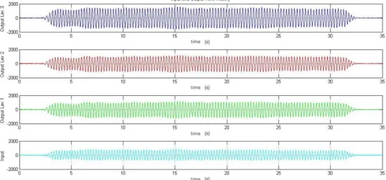
The data for the identification procedure are given by records of the absolute acceleration, reported in Figure 5 for a sample case (m0t5, in Table 3). .

time

time

time

time

Table 5 lists the identified modal parameters obtained by means of the classical

input-output Goyder procedure [2].

Mode frequency Hz damping ratio [%] modal displacements 1st floor 2nd floor 3rd floor

1 2.63 1.61 -0.605 -0.880 -1.377

2 6.79 1.63 -0.285 -0.177 0.283

3 9.63 2.40 -0.088 0.139 -0.048

Table 5: Modal parameters identified by the Goyder procedure for the case m0t5 of Table 3.

Based on the same experimental data of case m0t5, Table 6 reports the modal parameters identified by means of the output-only procedure described in Section 2; as a starting point of the error minimization, natural frequencies, damping ratios and modal constants fairly distant from those identified with the input-output technique have been assumed (30 % difference), in order to test the robustness of the procedure; the output-only solution has been found with the minimization algorithm described in Section 2.3, within the boundaries ± 30 % with respect to the reference solution, i.e. the solution identified with the Goyder procedure.

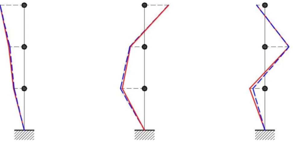
As shown by comparison between modal parameters in Table 5 and Table 6, the

output-only procedure, introduced in [1] and modified in [3] with an improved minimization

algo-rithm, provides, for the sample case described here, a good agreement with the classical

input-output procedure, as also shown by the comparison of modal shapes in Figure 6.

Mode frequency [Hz] damping ratio [%] modal displacements 1st floor 2nd floor 3rd floor

1 2.64 1.57 -0.664 -0.956 -1.590

2 6.79 1.52 -0.306 -0.194 0.330

3 9.64 2.36 -0.078 0.157 -0.054

Table 6: Modal parameters identified by the output-only procedure for the case m0t5 of Table 3.

Figure 6: Comparison between modal shapes identified via the Goyder procedure (red line, values of Table 5) and via the output-only procedure (blue line, values of Table 6).

5 CONCLUSIONS

This paper describes the first results of an experimental campaign on a 3-dofs shear-type frame model, carried out to validate the output-only procedure proposed by one of the writers [1] to identify the modal parameters of a structure subjected to unmeasured base motion.

The modal parameters are identified by means of a minimisation algorithm, improved from the computational point of view as described in [3]. The error function to be minimised com-pares, in the least square sense, the analytical relationships of the dynamic response and their experimental counterparts.

As shown by the results reported, the output-only procedure provides a good agreement with a classical input-output procedure.

A larger experimental campaign is currently in progress for the validation of the proce-dure. A particular attention will be given to all the uncertainties emerged in the present work, as for example the dependence of the identified modal parameters on their initial estimate and the boundaries, and on the intensity and the time-length of the imposed base motion.

ACKNOWLEDGEMENTS

The financial support of University “G. d’Annunzio” of Chieti-Pescara (MIUR ex 60% funds) is acknowledged by the authors.

REFERENCES

[1] V. Sepe, D. Capecchi, M. De Angelis, Modal model identification of structures under unmeasured seismic excitations, Earthquake Engineering and Structural Dynamics, 34: 807-824, 2005.

[2] H. D. G. Goyder, Methods and application of structural modelling from measured fre-quency response data, Journal of Sound and Vibration, 68: 209-230, 1980.

[3] V. Sepe, F. Iezzi, R. Siano, C. Valente, Validation of a Modal Identification Procedure for Linear Frames under Unmeasured Seismic Input, IEEE Workshop EESMS 2014, September 12-17, Naples, Italy, 2014.

[4] Brinker R., L. Zhang, Andersen P., Modal identification of Output-only Systems Using Frequency Domain Decomposition, Smart Materials and Structures, 10 (3), 441-445, 2001.

[5] Ewins D.J., Modal testing: theory and practice, Research Study Press –Wiley: Chiches-ter, 1996.

[6] M. De Angelis, V. Sepe, F. Vestroni, Identificazione dei parametri modali di una strut-tura eccitata alla base, Ingegneria Sismica, Anno XVIII n. 3, September – December 2001 (in Italian).