Remote sensing for monitoring and mapping land productivity in Italy. A rapid assessment methodology

REMOTE SENSING FOR MONITORING AND

MAPPING LAND PRODUCTIVITY IN ITALY

A rapi

d assessment methodol

ogy

M. SCIORTINO, M. DE FELICE Department for Sustainability Division Models and Technologies for Risks reduction Climate and Impact Modelling Lab Casaccia Research Centre

L. DE CECCO, F. BORFECCHIA Department for Sustainability

Division Protection and enhancement of the naturalcapital Laboratory for Observations and Analyses of

the Earth and Climate Casaccia Research Centre

RT/2018/14/ENEA

ITALIAN NATIONAL AGENCY FOR NEW TECHNOLOGIES, ENERGY AND SUSTAINABLE ECONOMIC DEVELOPMENT

M. SCIORTINO, M. DE FELICE Department for Sustainability Division Models and Technologies for Risks reduction Climate and Impact Modelling Lab Casaccia Research Centre

REMOTE SENSING FOR MONITORING AND

MAPPING LAND PRODUCTIVITY IN ITALY

A rapid assessment methodology

L. DE CECCO, F. BORFECCHIA Department for Sustainability

Division Protection and enhancement of the natural capital Laboratory for Observations and Analyses of

the Earth and Climate Casaccia Research Centre

RT/2018/14/ENEA

ITALIAN NATIONAL AGENCY FOR NEW TECHNOLOGIES, ENERGY AND SUSTAINABLE ECONOMIC DEVELOPMENT

I rapporti tecnici sono scaricabili in formato pdf dal sito web ENEA alla pagina www.enea.it I contenuti tecnico-scientifici dei rapporti tecnici dell’ENEA rispecchiano

l’opinione degli autori e non necessariamente quella dell’Agenzia

The technical and scientific contents of these reports express the opinion of the authors but not necessarily the opinion of ENEA.

REMOTE SENSING FOR MONITORING AND MAPPING LAND PRODUCTIVITY IN ITALY A rapid assessment methodology

M. Sciortino, M. De Felice, L. De Cecco, F. Borfecchia Riassunto

Presentiamo una metodologia basata sul telerilevamento per una rapida valutazione dello stato e delle tendenze della produttività del territorio (LP) a livello nazionale e subnazionale. Questa metodologia mira a sostenere le politiche ambientali nazionali e internazionali per raggiungere l'obiettivo di Land Degradation Neutrality nel quadro dell'Agenda 2030 delle Nazioni Unite e degli Obiettivi di sviluppo sostenibile. Il lavoro è stato eseguito utilizzando l'indice NDVI (Normalized Difference Vegetation Index) della NASA-MODIS come indicatore proxy dello stato e della tendenza di LP. Lo stato LP è stato identificato dalla media e dalla deviazione standard dei valori annuali LP 2000-2015. I trend di LP delle serie annuali sono state calcolate utilizzando i test Kendall (MK) e Contextual Mann-Kendal (CMK). La quantità di terreno con trend crescenti e decrescenti è stata valutata assumendo il livello di significatività del 95% nelle aree ove la qualità del dati NDVI è affidabile. L'area di trend LP crescenti e decrescenti è stimata per il territorio nazionale e per diverse coperture del suolo. Le varia-zioni di LP positive osservate sono sicumente correlate alla progressiva rinaturalizzazione del territorio in seguito alla diminuzione delle attività agricole e all'aumento delle precipitazioni nella stagione in-vernale nel periodo di riferimento. La diminuzione di LP ha interessato aree molto limitate correlate a variazioni delle precipitazioni stagionali e/o delle attività umane. I comuni maggiormente interessati dal declino o dall'aumento di LP vengono identificati allo scopo di individuare le aree ove possibilmente effettuare specifiche attività di monitoraggio e convalida future.

Abstract

We present a remote sensing-based methodology for rapid assessment of status and trends of Land Productivity (LP) at national and sub-national scales. This methodology aims at supporting environ-mental national and international policies to achieve the Land Degradation Neutrality target in the framework of the UN Agenda 2030 and the Sustainable Development Goals. The work was performed in Italy using the NASA-MODIS Normalized Difference Vegetation Index (NDVI) as proxy indicator of LP status and trend. LP status was identified by mean and standard deviation of 2000-2015 yearly LP values. LP trends of the yearly time series were computed using Mann-Kendall (MK) and Contextual MK (CMK) tests. The amount of land with valid increasing and decreasing trends is estimated assuming the 95% significance level of trends in the areas with good pixel reliability. The area of increasing and decreasing LP are estimated for the national territory and for different land covers. The widespread observed positive LP variations were correlated to the progressive renaturalization of lands subsequent to the decrease of agricultural activities and increasing precipitation trends in the winter season. LP decrease affected very limited areas and hot spots were correlated to changes of seasonal precipita-tion and human activities. The municipalities most affected by LP decline or increase are identified for future monitoring and validation activities.

1. Introduction 2. Data and Methods 3. Results

3.1 Land Productivity baseline 3.2 Land Productivity trends

3.3 Are precipitation changes a cause of LP changes? 4. Discussion 5. Conclusions 6. References 7. Supplementary S1 8. Supplementary S2 9. Supplementary S3 7 9 11 11 14 18 19 21 23 27 30 33 INDEX

7

1. Introduction

Land degradation and desertification are considered global threats to the sustainable development of many countries. This is the message that international policy makers agreed to stress at the RIO+20 United Nation Conference on Sustainable Development in June 2012, recommending countries and the international community to identify urgent actions to reverse the current land degradation trend.

In September 2015, the United Nations General Assembly adopted “The 2030 Agenda for Sustainable Development”, including 17 Sustainable Development Goals (SDG) and 169 targets. The target 15.3 introduced the concept of Land Degradation Neutrality (LDN) aiming to protect, restore and promote sustainable use of terrestrial ecosystems, sustainably manage forests, combat desertification, and halt and reverse land degradation. The indicator adopted by governments to measure the achievement of LDN is the “Proportion of land that is degraded over total land area”.

The United Nations Convention to Combat Desertification (UNCCD) endorsed the concept of LDN as a strong vehicle for driving the implementation of the Convention inviting all its country Parties to formulate voluntary national targets. UNCCD also suggested the countries to measure the progress in the implementation of their activities by three principal indicators, land cover and land cover change, land productivity and carbon stocks above and below ground in order to identify degraded, degrading and improving areas.

The Land Productivity (LP) indicator was intended to measure the total above ground Net Primary Productivity (NPP). This indicator, specifically addressed in this work, seems suitable for policy making support because of the availability of data and methods for its quantification. The spatial and temporal resolution of remote sensed data may provide continuous and synoptic information to identify the impacts of natural and anthropic pressures on the status and trends of vegetation cover.

The policy demand on LP monitoring and assessment can be satisfied by integrating remote sensing data, land cover data and other geographic data introducing a quantitative and statistically based approach in the desertification policy context.

Remote sensing data are recognized as the main resource for an extensive monitoring and mapping of LP and the Normalized Difference Vegetation Index (NDVI) is considered a suitable proxy for LP because is related to net primary productivity (NPP) (Seaquist et al., 2003, Scheftic et al., 2014) and to many biophysical parameters that control land-atmosphere fluxes and vegetation productivity (i.e. leaf-area index, fraction of photo-synthetically active radiation absorbed by vegetation, etc.) (Asrar et al., 1984, Myneni et al., 1995). Previous studies and projects addressed how to measure desertification and land degradation on the basis of spectral vegetation indices at national level (Del Barrio et al., 2010, , Eckert et al., 2015, Gaitàn et al., 2015). On a regional scale the European Space Agency launched in 2004 the DesertWatch project to develop an information system based on remote sensing for monitoring land degradation trends over time, focusing on Mediterranean countries (Portugal Italy and Turkey) (DesertWatch, 2012) using the satellite

8

MERIS data. Global and continental land degradation studies were based mainly on NOAA AVHRR data (Hellden et al., 1988, Bai et al., 2008) made available by the Global Inventory Modelling and Mapping Studies (GIMMS). Different methodological and statistical approaches have been applied to analyse NDVI data with spatial resolutions ranging respectively from 1 to 8 Km. The time frame from 1981 to 2003 of GIMMS data has been extended to 2010 for the European Region (Cherlet et al., 2013) by integrating the observational records with data from the SPOT Vegetation sensor. Despite the scientific understanding and data made available by international institutions, a gap between the policy demand of operational indicators and the availability of a user-oriented methodology is still open. The countries affected by desertification are requested by UNCCD to implement policies and actions over their territory and monitor the evolution of processes at national and sub national scales. Remote sensing is still insufficiently adopted by countries to detect trends for the identification of improving and degrading areas because of the insufficient communication between policy makers and science and technology institutions. The main issue addressed in this work is the demonstration of the usefulness of using remote sensing data, statistical modelling and Geographic Information System (GIS) for an updated quantitative reliable methodology for the monitoring of the LP status and trends, as well as the identification of the areas affected by land degradation at country level. The assessment methodology we present, aims to make progress toward this direction and support policy makers for the identification of policies and actions requested for the implementation of UNCCD and SDG’s targets.

9

2. Data and Methods

Satellite data

The NASA MODIS archive (https://lpdaac.usgs.gov/data_access/data_pool) provides global data for spatial and temporal evaluations of vegetation status and changes. Global NDVI data from the Terra and Aqua platforms are provided every 16 days as gridded Maximum Value Composite (MVC) at 250 meter spatial resolution (Holben 1986).

The 1,472 MVC tiles for the years from 2000 to 2015, covering the Italian territory (spanning over 4 tiles), were downloaded, re-projected and mosaicked using the implemented ‘ModisDownload’ function in R and the MODIS Reproject Tool (MRT) software.

Precipitation data

Precipitation monitoring station data in Italy are collected by a number of national and regional services for meteorological, hydrological, agro-meteorological purposes. Harmonization and standardization of the data of different networks was made for climate change studies (Desiato et al., 2007; Desiato et al., 2011). Although the station data are made available by regional monitoring services through their web sites the only data storage and retrieval service at national scale is organized and provided by SCIA (National System of collection, elaboration and distribution of Climate data: http://www.scia.isprambiente.it) as station and 5 km gridded monthly data archive. The yearly and the monthly cumulated precipitation values for the years 2000-2015 have been downloaded and analysed for the detection of trends and to be correlated with LP changes. The analysis of annual cumulated precipitation, standard deviation and annual and seasonal trends are shown in the supplementary section S1.

Land cover

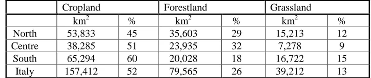
The Corine 2012 land cover data (CLC2012), distributed by the Istituto Superiore per la Protezione e la Ricerca Ambientale (ISPRA) and by the European Environment Agency (EEA), having an accuracy greater than 100 m and a minimum mapping unit of 25 ha, represent the best available option for the land cover mapping in Italy. The geographic distribution of the land cover classes, cropland, forestland and grassland, obtained aggregating the CCL2012 data according to the IPCC land categories (IPCC 2006), represents the 91% of the national land cover (Table 1).

10

Cropland Forestland Grassland

km2 % km2 % km2 %

North 53,833 45 35,603 29 15,213 12 Centre 38,285 51 23,935 32 7,278 9

South 65,294 60 20,028 18 16,722 15 Italy 157,412 52 79,565 26 39,212 13

Table 1. Extension of cropland, forestland and grassland in the three Italian macro regions.

Cropland is the dominant class found mainly on plains, coasts and islands of southern regions. The more ‘‘natural’’ land-use/land-cover classes (e.g., forestland and grassland) is found mostly in the mountain areas of central and northern regions. The extension of cropland in southern regions is greater than in other regions while forestland is the prevalent in the central and northern regions. Other land cover classes (settlements, wetlands, other land and bare land), representing 9% of the national territory, are not included in this study because vegetation cover density might be insufficient for the interpretation of changes of LP on the basis of remote sensed indices. Changes in land cover are also important indicators in their own as they provide an indication of the soil sealing due to the expansion of settlements that is considered one of the most relevant of land degradation processes in Italy. Using the CLC data the changes of the IPCC land cover classes, cropland, forestland, grassland, settlements, wetlands and other lands, have been estimated. From the year 2000 to 2012 urban areas increased by 813.6 km2 and forestland cropland decreased respectively by 442 and 730 km2. The land cover layers of forestlands, croplands and grasslands in 2012 have been used to stratify the LP data and therefore the analysis of the changed areas are excluded from this study.

Data processing

For each year, 23 MVC layers were stacked into a single annual multilayer file in order to generate the 16 years’ time series of NDVI annual mean for the Italian territory. The pixel reliability information provided by NASA for all NDVI files has been used for computing the reliability index and identifying the areas with good data for the detection of LP trends.

The methodology and the results of the reliability analysis are described in the supplementary section S2. The trend sign and significance for each individual pixel in domain is first estimated using the Mann-Kendall (MK) non parametric tests (Kendal 1962), assuming that data values full fill the condition of independence between observations with no tied data values (Douglas, 2000). The MK test has been applied also to annual and seasonal precipitation data.

Because of possible temporal and spatial autocorrelation of data, the MK result may overestimate the real number of valid trends pre-processing of data and Contextual Mann-Kendall (CMK) are used (Neeti et al., 2011). The temporal auto correlation may be induced by a random perturbation affecting the annual mean value and its influence may persists for an unknown length of time. The annual mean values may be influenced by its past history by processes such as recovery from the sudden impact of a forest fire that is

11

expected to take several years. Prewhitening is used to eliminate the influence of temporal auto correlation on the test of trends. The process of prewhitening involves the computation of the serial correlation coefficient (ρ) and the application of an iterative process until the coefficient is below the prescribed threshold (ρ <0.05) (Neeti et al., 2011).

Spatial cross-correlation may also affect the detection of valid trends under the case of spatial dependence between neighbouring pixels leading to the identification of statistically significant trends while it is not true. NDVI data may be subject to perturbations causing isolated pixels with significant trends. However, the absence of similar trends at immediately neighbouring pixels reduces one’s expectations that such isolated trends are something other than chance occurrences. In addition, if the sample size of the time series is small, then there are chances of having trends that are only marginally significant even if immediate neighbouring pixels exhibit similar trends. In such cases, one’s expectation of similar behaviour between neighbours would lend greater confidence in the presence of a trend. The occurrence of isolated trend may be removed applying the Contextual Mann-Kendall (CMK) test evaluating the trends comprised in the region of 3 by 3 neighbourhood around each pixel and adjusting the variance during significant trend testing. (Neeti, et al., 2011).

In order to test the impact of temporal and spatial autocorrelation on the number of valid positive and negative trends three tests have been applied in this study:

1) MK tests without any pre-processing of time series data,

2) CMK test after removing the effect of temporal auto correlation.

The two statistical tests, described in the supplementary section S3, provide a range of values for the areas with positive and negative trends that will require validation field studies.

Autocorrelation and cross correlation of precipitation data is not considered in this study because the data utilized are not station data but interpolation of station data on a regular grid.

Data processing for trend and mapping is made using the R statistical package (version 2.14.1; http://www.r-project.org/) and IDRISI Earth Trend Modeler (https://clarklabs.org/terrset/earth-trends-modeler/).

3 Results

3.1 Land Productivity baseline

LP baseline, based on the estimation of the LP temporal mean (LPav) and standard deviation (LPsd) of the 16 years annual NDVI observations, reflects the temporal and spatial variability of land conditions due to natural and anthropic effect on vegetation cover.

The geographic distribution of LPav and LPsd values is determined by many factors including climate, land morphology and land cover. High, medium high, medium low and low LP areas have been identified using the 25°, 50° and 75° percentile thresholds of LPav and LPsd cumulated distributions for cropland, forestland and grassland (Figure 1).

12

Figure 1. Maps of Mean and Standard Deviation of the Land Productivity Index

The patterns of the two maps clearly highlight: croplands characterized by large mono-cultures, intensely ploughed before seeding and after harvest with little strip of vegetation left in-between, having limited average standing biomass and high peak values during a relatively short growing period. The low LPav cropland areas, especially in the South (Sicily, Sardinia, Puglie) show medium high LPsd, which points to a relatively high inter annual variability of LPav, which could perhaps also be caused to crop rotation and/or impact of climate variability. A field validation would be necessary to identify where the signal of instability can qualify for a critical LP status.

The areas turned before the year 2000 practically to barren land, strongly dominated by urban and artificial structures, are associated to low LPav and low LPsd.

The north western regions, where rice cultivation is made with seed setting in the water, which results in low NDVI even in the early growth period show “low LPav” and quite stable yields , which results in “low LPsd” .

The protected forest or semi-natural areas characterized by high LPav and low LPsd, (e.g. the protected evergreen forest in the Gargano park in Puglia, or in the Calabrian Aspromonte and forest in the Apennine mountains).

13

The alpine region in with low LPav and high LPsd where the presence of seasonal snow and frequent cloudy conditions significantly affect the vegetation index reliability as shown in the supplementary data S2.

The variables of LPav and LPsd seem to be meaningful and promising to measure LP actual conditions of specific land cover areas and/or within administrative and geographic boundaries The LPav LPsd indices may be a useful proxy to detect the different land conditions within the same land cover class and can provide a large scale measure of land conditions. They are based on the detection of land greenness and may represent a quantitative measure of land properties that can be used as elements for the evaluation of the time change of the yearly LP in respect to long term baseline.

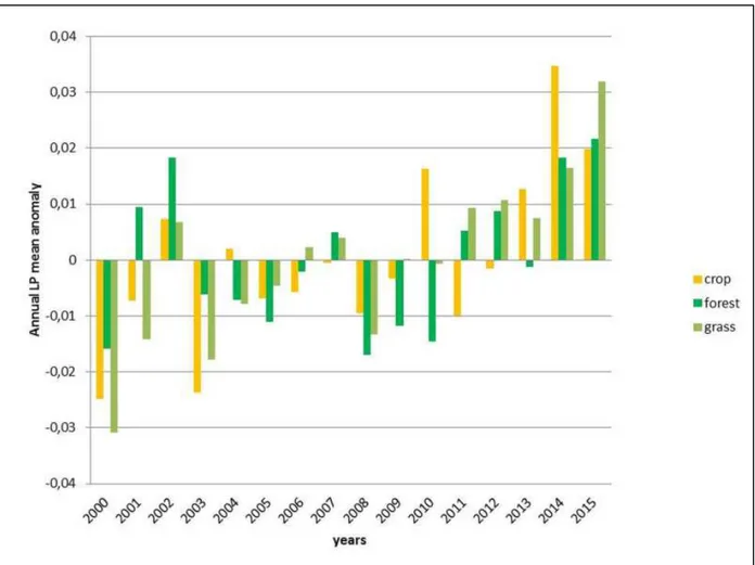
Figure 2. Land Productivity Index year anomalies in Italy for cropland, forestland and grasslands

The LP yearly anomalies for the three layers show a marked positive trend in all three land covers providing a first qualitative evaluation of the changes at national scale. The positive anomaly change at national scale indicate that all three land covers, increased their greenness due to a combination of factors that will be discussed in the following paragraph. Yearly LP anomalies might be used for geographic or administrative subnational boundaries to check the occurrence of sub national anomalies to be validated with field studies.

14

3.2 Land Productivity trends

Setting the LP baseline, as described in the previous paragraph, is a stock-taking exercise where a snapshot of the current land-based natural capital is taken; it does not provide any information on the current land productivity change in the individual spatial units. A retrospective assessment of LP trends (LPtr) is an essential step in terms of understanding current conditions of land productivity, revealing anomalies and possible degrading areas at the spatial resolution of the available data. Trends assessment, within the limits of the sensitivity of the non-parametric tests (Wessels et al., 2012), aims to provide an informed evidence base for setting sound policy targets, making decisions about potential interventions and prioritizing efforts in areas where land productivity change is taking place.

The quantitative estimation of the area affected by LP change is made for croplands, forestlands and grasslands as identified by the CORINE 2012 database.

The areas with significant trends (p<0.05) according to the different statistical tests applied is (Table 2).

15

Table 2. Areas of significant (p<0.05) Land Productivity trends of annual mean NDVI using Mann-Kendall (MK) and Contextual

Mann-Kendall (CMK) with adjustment of temporal autocorrelation.

The significant trends (positive and negative) with MK test at pixel level without pre-processing of time series are 28% of the total while the significant trends with CMK test after pre-processing for removing the effect of temporal autocorrelation are 38%.

The number of significant trends with the CMK tests, after data pre-processing, increased by 10% decreasing the number of negative trends (-82%) and increasing the number of positive trends (+44%).

The CMK significance test for removing the spatial autocorrelation, decreases the number of negative trends occurring in isolated pixels in areas with no neighbouring significant trends and to increases the number of positive trends occurring in areas were marginally significant trend become significant because of the adjustment. This change reflects the expectation that similar behaviour between neighbours, although marginally significant, may give greater confidence in the presence of a significant trend. The CMK test is conservative for the identification of the negative trends that are the primary concern of land degradation but, although the less conservative, MK tests identifies the same areas with clustered negative trends.

MK test CMK test

Positive Negative Positive Negative

Cropland (km2) 45,739 2,789 66,699 377 Forestland (km2) 13,802 1,821 20,760 414 Grassland (km2) 13,332 177 17285 27 Total (km2) 72,873 4,787 104,744 818

16

Figure 3. Geographic distribution of the valid LP trends, by region (A) and by land cover (B).

The geographic distribution of the valid LP trends, according the CMK test shows that the positive trends prevail in southern regions and negative trends prevail in northern regions (Figure 3a) and that the norther and central forests are the most affected land cover by negative trends (Figure 3b). The areas with LP decline and LP increase above the selected thresholds aggregated at municipality level (Figure 4) are used to identify hot spots over the national territory.

17

Figure 4. Geographic distribution of LP trends hot spots.

Although croplands show general positive LP trend across the southern Italian regions (Figure 3b), the decreasing LP-hot spots in southern regions affect croplands. The causes of the LP negative hot spot in the municipalities in the Calabria region may be attributed to seasonal (April-May-June) precipitation decline (Supplementary S1). The ”hot spots” of LP decrease in Sicily, Campania and Lazio croplands might be explained by crop changes or by other anthropogenic causes to be identified. The LP negative trends hot spots in Tuscany, Liguria and Piedmont regions affect forestlands and climatic forcing emerged from the analysis of precipitation data in the time frame of this study.

18

Although the quantity of land affected by negative trend areas is limited the methodology may provide indication to land managers and policy makers on ongoing process and support monitoring activities to be conducted locally.

3.3 Are precipitation changes a cause of LP changes?

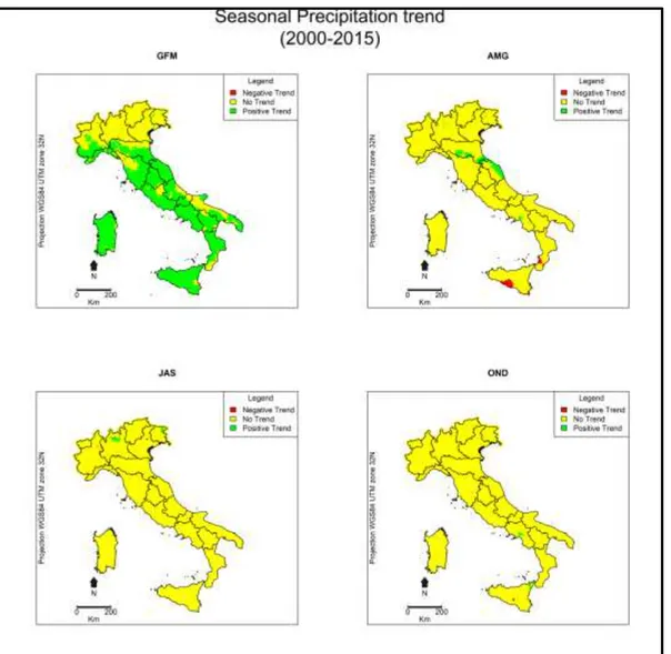
Precipitation trends for seasonal and annual cumulated precipitation for the years from 2000 to 2015 have been computed according to the MK test. The statistically significant (p<0.05) annual and seasonal trends show increasing rainfall in winter and spring months and no evidence of negative trends in the 16 years data records (Supplementary material S1). The positive trends of annual and seasonal (DJF) precipitation provide a first qualitative correlation between the prevalent greening of vegetation and the concomitant climate conditions.

The statistical correlation test is made using the multiple linear regression model. The linear regression equation best fitting LP temporal records:

𝐿𝑃 = 𝑘₁∗ 𝑇 + 𝑘₂∗ 𝑃 + 𝑘₃∗ 𝑓(𝑇, 𝑃) + 𝑘₄

where T is the time (year), P the annual cumulated precipitation, 𝑓(𝑇, 𝑃) a function of time and precipitation, is used to identify the pixels where the correlation between LP and the predictors is significant (p<0.05) on the basis of the Akaike Information Criterion (Akaike Information Criterion, Wilks, 2011). The predictors, time, precipitation and their combination are significant respectively in 28%, 18%,15% of the national territory. No significant correlation of LP with the predictors is found 38% of the territory (Figure 5).

19

Figure 5. Geographic distribution of significant NDVI correlations.

The multiple linear regression methodology results identified larger areas of significant correlation in respect to the Pearson methodology. This result could be improved at regional and local scale by using station data records collected from regional meteorological services. In conclusion only 18% of the annual LP changes seems to be correlated to precipitation changes and 28% of the changes can be attributed to progressive changes correlated to anthropic activities, especially land use change and land abandonment. The seasonal or monthly scale analysis should be also addressed in future studies to take in account process the cannot be identified at annual scale.

4. Discussion

The estimation of trend of annual mean values is critically dependent on the spatial resolution and the applied statistical method. The analysis of 16 years of NASA-MODIS data represent a progress in respect of previous results based on NOAA-AVHRR data because of the improved spatial resolution. Previous studies mainly addressed the detection of trends at global (Bai, 2008) and continental scale (Cherlet, 2013). Comparing this study results with results of previous works is impossible because of the different spatial and temporal frames.

Previous studies of monitoring and assessment of land degradation in Italy (Salvati et al. 2016) using the Environmental Sensitive Area (ESA) methodology identified critical areas and the progressive increase of the ESA index over the Italian territory. The ESA most sensitive areas (i.e. southern Italy, Sicily and Sardinia, Po valley and other areas on the east cost of Italy in their Figure

20

1) correspond to the low annual mean LP areas in Figure 1 of this paper. The ESA vulnerable areas, defined as a desertification hotspot remained stable from 1960 to 2010, because of locally increasing climate quality and land-use changes mitigating desertification processes such as natural forestation and decreasing population pressure(Salvati et al. 2016). This result is supported by the LP trend results reported in this study that show a general increasing trend. On the contrary, the sensitivity of previously ESA ‘non-affected’ areas (mainly concentrated in northern and central Italy) is identified by Salvati as rapidly increasing during the investigated time period, suggesting that important variations have occurred in climate and socioeconomic conditions in this region. Salvati also claims that sensitivity of land degradation in northern Italy will be higher in future than in the past. The results shown in figure 4 support similar conclusions regarding the LP improving condition limited to central and southern regions.

The results presented in this paper using a remote sensing based diagnostic methodology confirm some previous findings such as the improved vegetation condition of Italian southern regions and islands and decreasing trend of LP in northern regions.

The methodology adopted in this work is not entirely new but there is an innovative approach based on near real time remote sensing data, statistical confidence thresholds, reliability indices and use of open source tools that might significantly improve the contribution of science to desertification policy.

The map of LP status baseline developed in this study, enabled to identify the geographic distribution of high, medium, low productivity areas and the annual anomalies of LP mean values between year 2000 and 2015, in Italian croplands, forestlands and grasslands. The LP trends, assumed as proxy indicator of increasing and decreasing “Land Productivity” associated to quantity of biomass and the quantity of carbon stored in the vegetation, provide a range of values of the areas interested by significant positive and negative changes. The results obtained from trend analysis and from annual mean anomalies confirmed that that Land Productivity was by large the prevailing change identified in this study as also diagnosed by the last national forestry (INFC, 2015) and agriculture (ISTAT, 2013) inventories.

21 5. Conclusions

The Normalized Difference Vegetation Index, has been widely criticized because of its sensitivity to a wide range of perturbing effects unrelated to plants (e.g. atmospheric composition, soil moisture, surface anisotropy and non-optimal relations to vegetation properties) and for its limitations in densely vegetated regions, because of saturation effects (Myneni et al., 1995) that may, in certain vegetation types, cause NDVI not fully follow the photosynthetic cycle. Therefore, the results presented in this study should be interpreted with appropriate caution, although the interpretation of NDVI annual mean long-term trends can be expected to largely alleviate these concerns.

The LP assessment methodology represents, especially in desertification affected country parties of UNCCD, a promising tool that can be implemented to develop national monitoring capacities through appropriate initiatives and scientific cooperation. The availability of a science-based approach providing a quantitative methodology for the rapid assessment of LP status and trends at national and sub national scale might respond to the policy makers demand of a low cost diagnostic tool to be used for the monitoring of the evolution of terrestrial ecosystems. Remote sensing is a monitoring tool still insufficiently used to support national and international land degradation and desertification policies.

The use of remote sensing data does not replace field studies for the assessment of land degradation because LP decrease or increase cannot be directly associated to degradation or improvement of land. National and local circumstances such as land abandonment or land use change, bush and tree encroachment, identified by positive LP trends, may represent for local stakeholders a loss of natural capital or biodiversity, therefore local validation studies and stakeholders participation activities should be made before any consideration of possible adaptation policies and actions. In Italy the reported continuing increase of LP, due to the progressive reduction of agro pastoral activities and the abandonment of marginal agricultural areas where a massive re-naturalization process is taking place is the dominant change. The LP decline, although of limited extension, should be considered an early warning of land degradation and stimulate local studies with higher resolution data for the identification of appropriate policy advice and actions.

22

Acknowledgements

The MOD13Q1, MODIS Vegetation Index Global 250m, data product was retrieved from the online Data Pool, courtesy of the NASA Land Processes Distributed Active Archive Center (LP DAAC), USGS/Earth Resources Observation and Science (EROS) Center, Sioux Falls, South Dakota, https://lpdaac.usgs.gov/data_access/data_pool."

The precipitation data products were retrieved from the online SCIA data service, courtesy of ISPRA , http://www.scia.isprambiente.it/home_new.asp.

The UNCCD activities on “Land Degradation Neutrality” have been an important motivation to undertake this work. The authors wish to acknowledge the colleagues Lorenza Daroda, Giuseppe Scarascia Mugnozza, Stefan Sommer, Anna Luise, Michele Munafò and Alain Retiere for the comments and fruitful discussions on the paper topics.

Conflicts of interests

All authors declare that have no conflicts of interests that might be perceived as influencing their objectivity.

23 References

Asrar, G. E., Fuchs, M., Kanemasu, E. T., & Hatfield, J. L. 1984. Estimating absorbed photosynthetic radiation and leaf area index from spectral reflectance in wheat. Agronomy Journal,76: 300–306.

Bai Z. G., Dent D. L., Olsson L., Schaepman M. E. 2008. Proxy global assessment of land degradation. Soil Use and Management, 24: 223–234. DOI:10.1111/j.1475-2743.2008.00169.x

Borfecchia, F., De Cecco, L., Dibari, C., Iannetta, M., Martini, S., Pedrotti, F., & Schino, G. 2001. Ottimizzazione della stima della biomassa prativa nel parco nazionale dei monti sibillini tramite dati satellitari e rilievi a terra. In Atti del V Congresso nazionale ASITA: 9-12

Brunetti M, Maugeri M, Monti F, Nanni T. 2006. Temperature and precipitation variability in Italy in the last two centuries from homogenised instrumental time series. International Journal of Climatology 26: 345–381.

Cherlet M., Ivits E., Sommer S., Toth G., Jones A., Montanarella L., Belward A. 2013. Land Productivity Dynamics in Europe. EUR 26500 EN, EUR. Scientific and Technical series. 2013 54 pp. ISBN 978-92-79-35427-4 ISSN 1831-9424 (online)

(http://wad.jrc.ec.europa.eu/data/EPreports/LPDinEU_final_no-numbers.pdf last accessed 02/03/2015)

CORINE Land Cover: http://www.eea.europa.eu/publications/COR0-landcover;

Del Barrio G., Puigdefabregas J.,. Sanjuan M.E, Stellmes M., Ruiz A. 2010. Assessment and

monitoring of land condition in the Iberian Peninsula, 1989–2000, Remote Sens. Environ., 114 , pp. 1817–1832

Desiato F., Lena F., Toreti A. 2007. SCIA: a system for a better knowledge of the Italian climate, Bollettino di Geofisica Teorica ed Applicata, 48(3): 351-358.

Desiato F., Fioravanti G., Fraschetti P., Perconti W., Toreti A. 2011. Climate indicators for Italy: calculation and dissemination. Advances in Science and Research, 6: 147-150. doi:10.5194/asr-6-147-2011.

24

Desiato F., Fioravanti G., Fraschetti P., Perconti W., Piervitali E. 2012. Elaborazione delle serie temporali per la stima delle tendenze climatiche, Rapporto ISPRA Serie Stato dell’Ambiente n. 32/2012.

DesertWatch, 2012. http://dup.esrin.esa.it/files/131-176-149-30_2009430103852.pdf (accessed on 11/01/2018)

Douglas E, Vogel R, Kroll C., 2000. Trends in floods and low flows in the United States: Impact of spatial correlation. Journal of Hydrology 240: 90–105

Falcucci A., Maiorano L., Boitani L.2007. Changes in land-use/land-cover patterns in Italy and their implications for biodiversity conservation, Landscape Ecol. 22:617–631 DOI 10.1007/s10980-006-9056-4.

Eckert S., Hüsler F., Liniger H., Hodel E., 2015. Trend analysis of MODIS NDVI time series for detecting land degradation and regeneration in Mongolia, Journal of Arid Environments, Volume 113, 2015, Pages 16-28, ISSN 0140-1963, https://doi.org/10.1016/j.jaridenv.2014.09.001.

Forest Europe, UNECE, FAO, 2011, State of Europe’s Forests 2011. Status and Trends in Sustainable Forest Management in Europe. Ministerial Conference on the Protection of Forests in Europe; ISBN 978-82-92980-05-7.

Forkel M., Carvalhais N, Verbesselt J., Mahecha M.D., Neigh C.M.D. and Reichstein M.,2013, Trend Change Detection in NDVI Time Series: Effects of Inter-Annual Variability and

Methodology,

Remote Sens., 5, 2113-2144; doi:10.3390/rs5052113

Gaitan, J.J.; Bran D., Azcona D.E., 2015. Trend of NDVI in the period 2000-2014 as indicator of land degradation in Argentina: advantages and limitations. AgriScientia, [S.l.], v. 32, n. 2, p. 83-93, 2015. ISSN 1668-298x.

Helldén U. and Eklundh L. 1988. National drought impact monitoring : NOAA NDVI and precipitation data study of Ethiopia. Lund, Sweden : Lund University Press.

25 Hansen M. C., Potapov P. V., Moore R., Hancher M., Turubanova S. A.,. Tyukavina A,. Thau D, Stehman S. V., Goetz S. J., Loveland T. R.,. Kommareddy A, Egorov A., Chini L., Justice C. O., G. Townshend J. R. 2013. High-Resolution Global Maps of 21st-Century Forest Cover Change. Science, 342: 850-853. DOI: 10.1126/science.1244693

Holben B. N. 1986. Characteristics of maximum-value composite images from temporal AVHRR data. Int. J. Remote Sensing, 7(2): 1417-1434

INFC 2015 Italian national forest inventory, http://www.sian.it/inventarioforestale/

ISTAT 2013, 6° Censimento Generale dell’Agricoltura, http://censimentoagricoltura.istat.it/

Kendall M G 1962 Rank Correlation Methods. New York, Hafner

Myneni R. B., Hall F. G., Sellers P. J., Mashak, A. L. 1995. The interpretation of spectral vegetation indexes. IEEE Transactions on Geoscience and Remote Sensing, 33: 481–486.

Neeti N., Eastman J. R. 2011. A Contextual Mann-Kendall Approach for the Assessment of Trend Significance in Image Time Series. Transactions in GIS, 2011, 15(5): 599–611

Salvati L., Scarascia M. E., Zitti M., Ferrara A., Urbano V., Sciortino M., Gipponi M. 2009. The integrated assessment of land degradation, Ital. J. Agron., 4 (3):77–90. DOI: http://dx.doi.org/10.4081/ija.2009.3.77

Salvati L., Zitti M., Perini L. (2016), Fifty years on: long term patterns of land sensitivity to desertification in Italy. Land degradation & development. 27:97–107

Scheftic W., Zeng X., Broxton P., Brunke M. 2014. Intercomparison of Seven NDVI Products over the United States and Mexico. Remote Sens., 6 :1057-1084; doi:10.3390/rs6021057

Seaquist, J.W.; Olsson, L.; Ardo, J.. 2003. A remote sensing-based primary production model for grassland biomes. Ecol. Model., 169:1311//f

26

Toreti A., Fioravanti G., Perconti W., Desiato F., 2009. Annual and seasonal precipitation over Italy from 1961 to 2006, International Journal of Climatology 29: 1976–1987

UNEP, 1997. in: Middleton, N. and D. Thomas, (Eds.), World Atlas of Desertification, Arnold, London, p 182

Wessels K.J., Van den Bergh F., Scholes R. J. 2012. Limits to detectability of land degradation by trend analysis of vegetation index data. Remote Sensing of Environment, 125:10–22.

27 Supplementary material on precipitation trends in Italy (S1)

In Italy, the very complex topography and its geographical position make the precipitation analysis difficult; the long term changes of precipitation in Italy have been investigated using 111 series from 1865 to 2003 (whereof 75 covering at least 120 years) (Brunetti et al.,2006) and using time series from 1961 to 2006 (Toreti et al., 2009) investigating annual and seasonal precipitation trends over Italy.

from a set of stations homogeneously distributed over the Italian territory, belonging to the Air Force Weather Service and to a few regional environmental protection agencies (ARPA).

Precipitation trends in this study do not aim to address climate change but the possible correlation with vegetation trends as identified from remote sensing Vegetation Indexes. Precipitation trends are computed from monthly cumulated precipitation values of stations interpolated on a 5 by 5 km grid by kriging. The interpolated data have been downloaded from the SCIA (National System of collection, elaboration and distribution of Climate data(Desiato et al., 2007).) dedicated we site http://www.scia.isprambiente.it). The station utilized to produce the interpolated data come from different national and regional meteorological networks and their number is 2426 in January 2000 but subject to variations according to the changing availability of station data from the year 2000 to 2015.Data were collected and controlled through SCIA before their interpolation and availability for downloading.The analisys of the annual and seasonal trends of cumulated precipitation values are estimated using the Mann-Kendall (MK) tests. The MK non parametric test (Kendal 1962) is used to identify for each individual pixel annual mean cumulated precipitation time series the trend sign and statistical significance. Assuming that data values full fill the condition of independence between observations with no tied data values the results shown in figure S1 and S2 are based on the the number of valid trends at 95% significance level for the annual and seasonal precipitation.

The areas with annual cumulated precipitation positive trends are identified in 11% of the national territory. No negative trend is identified in for annual cumulated values in the 2000-2015 time frame.

The seasonal cumulated precipitation might highlight patterns of trends that could be relevant for the interpretation of vegetation changes more than annual cumulated trends. The seasonal cumulated precipitation (Figure S2) shows increasing trends in January, February, March (GFM) and April, May, June (AMG). The areas with negative trends in southern Italy in AMG are the only of possible interest. The spatial correlation of AMG seasonal negative hot spots will be addressed using the Pearson and the multiple linear coefficient model. The small negative hot spot in other

28

seasons although not significant at national scale should be addressed using regional or local studies.

Figure S1, Annual cumulated precipitation trends from the year 2000 to 2015, according to MK significance test (p-value<0.05)

29

30

Supplementary material on data reliability analysis (S2)

Terra and Aqua MODIS NDVI form an important part of a long continuing record (Huete et al., 2011, Huete et al., 2002) begun with the Advanced Very High Resolution Radiometer, (AVHRR) and European Space Agency SPOT satellite and expected to continue with Copernicus Sentinel constellation satellites.

The data utilized in this work consists of data products derived from the Terra and Aqua MODIS sensors having 250 meters spatial resolution and 16 days frequency obtained by Maximum Value Composite (MVC) technique. The Terra and Aqua MODIS MVC data products are provided with two Quality Assessment (QA) layers:

250 m 16 days pixel Quality 250 m 16 days Pixel Reliability QA

The first layer contains pixel-level QA information and the second layer provides a summary pixel reliability QA. The Pixel Reliability layer provides simple ranks that capture the overall pixel quality. The pixel reliability data rank for each layer is:

Pixel Reliability Rank

(PRR)

Summary QA Description

0 Good data Use with confidence

1 Marginal data Useful, but look at other QA information

2 Snow/Ice Target covered with snow/ice

3 Cloudy Target not visible, covered with cloud

The pixel Reliability data ranks available for the 368 (16 days) layers can been used directly to interpret data reliability unlike the per-pixel Quality layer that requires detailed post-processing and interpretation. The 368 Reliability layers have been summed to compute and map a Pixel Reliability Index (PRI) for the entire study observation time frame.

The frequency of occurrence the different classes of Pixel Reliability Index over the Italian territory is:

31 PRI range counts

0 5 15,141 5 50 966,777 50 100 1,588,117 100 150 1,060,462 150 200 377,769 200 250 284,701 250 300 164,709 300 1000 366,444

The pixels in the PRI map (Figure S1) are classified in the unreliable data class when include records with snow/ice (PRR=2), clouds (PRR=3) and areas with marginal reliability (PRR=1) occurring more than 184 times in the pixel time record.

The good data quality class includes all PRR=0 and the PRR=1 if the Pixel Reliability Index is less than 184.

The area with unreliable data for the study of trends is 24,014 km2 mainly located in the mountain areas but also including some coastal areas and also croplands where land is flooded for rice cultivation.

32

Figure S2. The area of unreliable pixel data (24,000 km2) not included in the computation of land productivity trends.

33 Supplementary material on methodology for trend estimation (S3)

Mann-Kendall test

The Mann-Kendall trend test examines the slopes between all pair-wise combinations of samples. In the Mann-Kendall test, the data are ranked with reference to time and each data point is treated as the reference for the data points in successive time periods. Kendall’s S (Kendall 1962) is defined as: 𝑆 = ∑ ∑ 𝑠𝑖𝑔𝑛(𝑥_𝑖 − 𝑥_𝑗 ) 𝑛 𝑗=𝑖+1 𝑛−1 𝑖=1 and 𝑠𝑖𝑔𝑛(𝑥_𝑖 − 𝑥_𝑗 ) = { +1 𝑖𝑓 𝑥_𝑖 − 𝑥_𝑗 > 0 0 𝑖𝑓 𝑥_𝑖 − 𝑥_𝑗 = 0 −1 𝑖𝑓 𝑥𝑖 − 𝑥𝑗 < 0

where n is the length of the time series data set and xi and xj are the observations at times i and j,

respectively. The Mann-Kendall statistic is non-parametric and robust against outliers. However, it should be noted that it is actually a test for the presence of a monotonic trend and not strictly a linear trend.

According to Mann (1945) and Kendall (1975), the statistic S is approximately

normal when n ≥ 8. When there is no tie between data values then the mean and variance is given by:

𝐸(𝑆) = 0

𝑉𝑎𝑟(𝑆) =𝑛(𝑛 − 1)(2𝑛 + 5) 18 = 𝜎

2

where σ is the standard deviation.

The standardized Z test statistic is computed by:

𝑍 = { (𝑆 − 1) √𝑉𝑎𝑟(𝑆) 2 𝑓𝑜𝑟 𝑆 > 0 0 𝑓𝑜𝑟 𝑆 = 0 (𝑆 + 1) √𝑉𝑎𝑟(𝑆) 2 𝑓𝑜𝑟 𝑆 < 0

34

The Z statistic follows the standard normal distribution with zero mean and unit

variance under the null hypothesis of no trend. A positive Z value indicates an upward trend whereas a negative value indicates a downward trend. The p value of an MK statistic S can then be determined using the normal cumulative distribution function (Yue and Wang 2002):

𝑝 = 0.5 − 𝜙(|𝑍|)

where ϕ denotes the cumulative distribution function of a standard normal variate:

𝜙(|𝑍|) = 1 √2𝜋 2 ∫ 𝑒 −𝑡₂2 |𝑍| 0 𝑑𝑡

If the p value is small enough, the trend is quite unlikely to be caused by random sampling. At the significance level of 0.05, if p ≤ 0.05, then the existing trend is assessed to be statistically significant.

Contextual Mann-Kendall test

Isolated pixels exhibiting significant trends and the absence of similar trends at immediately neighboring pixels reduces one’s expectations that such isolated trends may be due to chance occurrences. One of the most fundamental principles of Geography is that neighboring locations tend to exhibit similar characteristics also commonly known as Tobler’s First Law of Geography; Tobler 1970). In addition, if the sample size of the time series is small, then there are chances of having trends that are only marginally significant even if immediate neighboring pixels exhibit similar trends. In such cases, one’s expectation of similar behavior between neighbors would lend greater confidence in the presence of a trend. The modified version of the Mann-Kendall test could make use of spatial autocorrelation as a line of evidence.

This leads to a modification in the MK test to include geographical contextual information, and is referred here as the Contextual Mann-Kendall (CMK) test.

The CMK test evaluates the trend in the area comprised of the 3 by 3 neighborhood around each pixel computing the areal average by:

𝑆_𝑚 = 1 𝑚∑ 𝑆𝑗

𝑚

𝑖=1

35 neighbors with the central pixel. The mean and variance of (Sm) for iid (independent and identically distributed) time series records of length n and without ties are given by:

𝐸(𝑆_𝑚) = 0

𝑉𝑎𝑟(𝑆_𝑚) =𝑛(𝑛 − 1)(2𝑛 + 5) 18𝑚 =

𝜎2

𝑚

According to the central limit theorem, Sm is normally distributed for large m if calculated from iid

data. Hence, Zm can be expressed as:

𝑍𝑚 =

𝑆_𝑚 − 𝐸(𝑆_𝑚) 𝜎 √𝑚

However, because of cross-correlation, the inclusion of neighbors tends to reduce the variance in the significance testing leading to increased detection of false significant trends (Yue and Wang 2002). Therefore, bias in significance testing due to inclusion of neighbors needs is corrected by:

𝑉𝑎𝑟(𝑆_𝑚) = 1 𝑚2 [ ∑ 𝑉𝑎𝑟(𝑆𝑗) + 2 𝑚 𝑗=1 ∑ ∑ 𝐶𝑜𝑣(𝑆_{𝑗 ,} 𝑚−𝑗 𝑙=1 𝑚−1 𝑗=1 𝑆_𝑗+𝑙 )]

Where 𝐶𝑜𝑣(𝑆𝑗, 𝑆𝑗+𝑙) is the covariance between neighbors j and j + l and the pm value of the CMK

statistic Sm can then be determined using the normal cumulative distribution function: 𝑝_𝑚= 0.5 − 𝜙(|𝑍_𝑚|)

ENEA

Servizio Promozione e Comunicazione

www.enea.it

Stampa: Laboratorio Tecnografico ENEA - C.R. Frascati settembre 2018