Temporal studies of GRB light curves and neutrino flux prediction for multi-collision zone model

(1)

Temporal studies of GRB light curves

and neutrino flux prediction

for multi-collision zone model

Facoltà di Scienze Matematiche, Fisiche e Naturali Corso di Laurea Magistrale in Astronomia e Astrofisica

Candidate Angela Zegarelli ID number 1529762

Thesis Advisor

Prof. Antonio Capone

Co-Advisor Silvia Celli

(2)

Temporal studies of GRB light curves and neutrino flux prediction for multi-collision zone model

This thesis has been typeset by LA_{TEX and the Sapthesis class.} Author’s email: Angela.Zegarelli@roma1.infn.it

(3)

iii

Cosmic Rays

1.1 Introduction

In 1911 and 1912 Austrian physicist Victor Hess made a series of ascents in a hydrogen balloon to take measurements of radiation in the atmosphere. He was looking for the source of ionizing radiation1 _{that registered on an electroscope.}

Initially the prevailing theory was that the radiation came from the rocks of the Earth.

In 1911 his balloon reached an altitude of around 1100 m, but Hess found no essential change in the amount of radiation compared with ground level. Then, on 7 August 1912, in the last of seven flights that year, Hess made an ascent to 5300 m and found an increase of the ionization rate if compared to the sea level. His result was later confirmed by German physicist Werner Kolhörster; he took balloon measurements up to a height of 9300 m founding again an increase of the ionization up to ten times that at sea level (Figure 1.1). The intensity of the radiation, at a fixed altitude, was relatively constant, with no day-night or weather dependent variations. This was the evidence that the source for these ionizing rays came from above the Earth’s atmosphere and it was therefore confirmed unambiguously that an unknown radiation with an extreme penetrating power was causing ionization.

Hess had therefore discovered a natural source of high-energy particles coming from the outer space: Cosmic Rays (CRs) [74]. He shared the 1936 Nobel prize in physics for his important discovery, and cosmic rays became a useful tool in physics experiments.

1.2 Energy Spectrum

The Earth’s atmosphere is continually crossed by cosmic rays (primary CRs), uni-formly and isotropically, that interacting with the atmosphere nuclei originate the so-called secondary CRs. The energetic particles that arise from this process collide in turn with other nuclei producing a "cascade of particles", which is called Extensive

Air Shower (EAS) [26], as shown in Figure 1.2. Through several experiments one

can study these showers and draw conclusions on CR characteristics. However, one

1_{Radiation that carries enough energy to liberate electrons from atoms or molecules, thereby}

(6)

Figure 1.1. Variation of ionization with altitude. Left panel: Final ascent by Hess (1912),

carrying two ion chambers [74]. Right panel: Ascents by Kolhörster (1913, 1914) [82].

Figure 1.2. Schematic view of an air shower with separated hadronic, muonic and

electromagnetic component (from [119]).

have to take into account the rate at which the particles arrive, depending on their energy.

The flux of cosmic particles is steeply falling with increasing energy, in fact the differential cosmic rays spectrum2 _{is well described by a power law distribution}

over a wide energy range, from few hundreds MeV up to about a hundred EeV [58](Figures 1.3 and 1.4):

dN

dE Ã E

≠“_. _(1.1)

There are four regions in the spectrum, each characterized by a specific value of

2_{Number of particles per unit time and unit solid angle incident on a unit area surface orthogonal}

(7)

1.2 Energy Spectrum 3

Figure 1.3. All-particle spectrum of cosmic rays, with it’s two features, the knee and the

ankle.

the spectral index “ and connected at three points: the knee at ¥ 3 · 106 _{GeV, the} second knee at ¥ 3 · 108 _{GeV and finally the ankle at ¥ 5 · 10}8 _{GeV. Below the knee} “ _{¥ 2.7, steepening to “ ¥ 3.1 and then “ ¥ 3.3 until the spectrum flattens at the}

ankle, above wich “ ¥ 2.6 (Figure 1.4).

The trend of the CRs spectrum can be explained by assuming that the CRs reach these energies through the so called "first order Fermi acceleration mechanism" (see Section 1.4.2), which can explain a flux proportional to E≠2_{; at this point different}

effects change the spectrum in the observed one.

The lowest energy band is dominated by particles trapped in the solar wind3 _[54].

The variability of their rate follows the solar cycle. In fact, during periods of high solar activity the solar wind interacts with the incoming CRs, disturbing their propagation to the Earth and reducing the observed flux. Conversely, the CRs flux reaches its maximum during the periods of low solar activity. This phenomenon is known as solar modulation and has a cycle of about 11 years. In the second band the

(8)

Figure 1.4. All-particle spectrum of cosmic rays, reconstructed from air showers observed

by various experiments (from [23]). The differential energy spectrum has been multiplied by E2.7 _{in order to display the features of the steep spectrum that are otherwise difficult} to discern (the second knee at 1017 _{eV) [23]. The grey box is the region where direct} observations of cosmic rats have been made. AGASA measurements show events with energy Ø 1020 _{eV [116], in contrast with the GZK cut-off.}

confining effect due to the galactic magnetic field works by changing the spectrum. Beyond the ankle CRs can not be confined in the galaxy volume by the galactic magnetic field and so this break in the spectrum slope could mark the transition between galactic and extragalactic cosmic rays.

Above 1 EeV particles are considered to be of extragalactic origin, because the radius of curvature of their trajectories in the galactic magnetic field exceeds the size of the Galaxy. The origin of the particles beyond the knee is not yet understood. Several models have been proposed to explain the acceleration mechanism bringing CRs to these extreme energies. There are three most developed scenarios:

• A change of the propagation of galactic cosmic rays, corresponding to a more rapid particle escape from the Galaxy [106].

• A change of the acceleration mechanism is directly responsible for the knee. It is argued that the maximal energy of acceleration in supernova shock fronts corresponds to the knee energy (see e.g. [81]).

• Presence of only one or few sources (supernovae) nearby the Earth. The consequences of this assumption to the cosmic ray spectrum are developed in [51].

The flux is then strongly suppressed at energies above 4 · 1019 _{eV. For these reasons} Ultra High Energy Cosmic Rays (UHECRs) are a topic of high importance. Greisen

(9)

1.2 Energy Spectrum 5

Figure 1.5. Fluxes of nuclei of the primary cosmic rays as a function of the kinetic energy

per nucleus [35].

radiation (Cosmic Microwave Background, CMB), pointed out that the power law of CRs should not exceed the energy at which they start interacting with the CMB. The involved reaction (with threshold of about ≥ 6 · 109 _{GeV) is:}

p+ “CMB æ+

I

p+ ﬁ0

n+ ﬁ+ (1.2)

where protons p interact with remnant photons from the Big Bang, “CMB, via +

resonance producing a nucleon (either a proton or a neutron) and a pion that is either positively charged (ﬁ+_{) if a neutron is created or neutral (ﬁ}0_{) if joined by}

a proton. Below the threshold energy the proton attenuation length is 1000 Mpc, while above the threshold it is reduced only to 20 Mpc. Similar effect appears, at higher nuclei energies, also for heavier nuclei and it is known as GZK cut-off. It would limit propagation of UHECRs to distances of order 20 Mpc and within this distance no suitable astrophysical source is known.

However, measurements by Akeno Giant Air Shower Array (AGASA) experiment observed significant number of events above the GZK cut-off (11 events above 1020

eV) [116][109][113] but this is the only measure that does not seem to observe the GZK cut-off so far. Other experiments, like HiRes [34] and the Pierre Auger Observatory [14], made measurements in this energy region by confirming a reduction of the particle flux for energies above the GZK threshold. (Figure 1.4).

(10)

the CRs is consistent with the overall spectrum up to energies close to the knee. The study of the relative abundances of these elements gives information about the acceleration mechanisms at the source and the propagation mechanisms in the Interstellar Medium (ISM). Indeed, any theory explaining the features in the cosmic ray spectrum will be tied to the composition at the energy of the feature.

1.3 Composition

Through experiments performed at high altitude (with balloons like or satellites) it has been possible to determine the composition of cosmic rays in the energy range between 108 _{eV and 10}14 _{eV; for energies beyond 10}15 _{eV the flow is so small (as}

shown in Figure 1.3) which requires the use of large detectors, necessarily on the Earth’s surface, that allow to study the particle showers produced by the primaries.

Figure 1.6. Abundances of elements observed in the cosmic rays compared to the Solar

System abundances. Abundances normalized to the value of 100 for Carbon.

Experiments showed that CRs are composed by protons (H, 85%), – particles (He, 12%), electrons (2%) and the remaining 1% by photons, heavy nuclei and neutrinos [58]. Comparing this composition with the abundances of metals in the solar system (Figure 1.6) it is immediate to assume that a large fraction of cosmic rays is produced in stellar environments, and their interaction with the interstellar medium (ISM) is responsible for the differences between the two distributions. In fact, in the CRs, elements lighter as Li, Be and B are much more abundant, and Sc, Ti, V, Cr and Mn are among the heaviest ones. These elements are present in CRs since produced by the interaction of oxygen and iron atoms respectively with the ISM by means of spallation reactions.

(11)

1.4 Acceleration Mechanisms 7

At lower energies these measurements are easier than at highest ones, mainly because at high energy, when the particle fluxes can be studied only by analysing the extensive air showers induced by the primary CR interactions, the mass reconstruc-tion becomes difficult. For this reason the UHECRs composireconstruc-tion is still very much under debate. Some observations favor a transition towards heavier elements just before the cut-off [1], while other are also compatible with a pure proton composition [115].

1.4 Acceleration Mechanisms

The power law behavior of the energy spectrum observed by Earth (see Section 1.2) is most probably indicative of a power law acceleration spectra, while spectral features may be assigned to changes in the origin of particles and/or their propagation.

Energy spectrum produced by Fermi acceleration

Let consider the energy transfer E following a random collision involving particles. It is proportional to the energy of the particle itself:

E = ›E, (1.3)

where › is then the amount of increasing energy; after n collisions the energy of a cosmic ray becomes

En= E0(1 + ›)n (1.4)

and the number of cycles needed to reach it is

n= ln 1 E E0 2 ln(1 + ›). (1.5)

The probability that the particle is confined until it achieves an energy En is given by the ratio between the involved number of particles N and the initial one N0:

Pn= N

N₀. (1.6)

From Equation 1.6 and by using Equation 1.5 the following expression can be obtained: ln3N N₀ 4 = ln3E E₀ 4s , (1.7)

where s = ≠ ln P/ ln(1 + ›). Therefore, the differential energy spectrum is naturally described by a power law:

dN

dE Ã E

≠(1+s)_. _(1.8)

(12)

a valid process responsible for the particle energy gain. The general equation of motion for a charged particle is:

d

dt(“m˛v) = q( ˛E + ˛v_{◊ ˛}B

c ), (1.9)

where “ = 1/Ò1 ≠v2

c2 is the Lorentz factor, q, m and ˛v are the charge, mass, and velocity of the particle, respectively. Equation 1.9 shows magnetic fields themselves do not work and can not be directly responsible for acceleration. A charged particle can be accelerated (its speed is changed) by increasing its energy and this can only be done by electric field, which are generated by variable magnetic fields.

1.4.1 Fermi acceleration of the II order

In 1949 Enrico Fermi proposed an acceleration mechanism due to collisions between particles and "clouds" with magnetic field irregularities inside them (magnetic

mir-rors), moving isotropically in the interstellar medium [52]. After having crossed

several times regions with unevenness of the magnetic field, the energy of the particles increases because head on collisions are on average more frequent. The energy gain at every cloud reflection is equal to:

= _E E > ≥ 4— 2 3 . (1.10)

For this reason this mechanism is also known as Fermi acceleration at second order in — = v/c and it is actually not very efficient because the value in Equation 1.10 is too small.

Starting from this theory, another one was developed, in which interactions of particles with a hydrodynamic shock wave can possibly take place: the Fermi

acceleration of the first order, explained in the following Section 1.4.2. 1.4.2 Fermi acceleration of the I order

One of the several physicists that independently modified the study previously done by Fermi was Anthony Raymond Bell in 1978 [30]. He improved the efficiency of the acceleration mechanism by hypothesizing a transfer of energy caused by strong shock-wave fronts moving in the interstellar medium with supersonic velocity U ∫ cs, where cs is the sound speed in a material. Consider the upstream fluid, not yet reached by the shock, and the downstream one, already reached and exceeded by it. The shock front is a transition zone in which the velocity of the fluid quickly change because of the supersonic motion of the supernova ejecta. Particles can pass through the shock in either direction by starting a series of diffusion processes due to the local turbulent (irregular) magnetic field; they are then scattered and their velocity distribution rapidly becomes isotropic in the frame of reference of the moving fluid on either side of the shock. This process can happen several time causing the energy gain of the particles.

The explanation of this topic will be now addressed by following Bell’s paper (1978) [30] and the Longair discussion [94]. Let consider the reference frame in which the

(13)

1.4 Acceleration Mechanisms 9

Figure 1.7. Cartoon picture of Fermi acceleration of the Second type. A schematic typical

path of a shock-accelerated particle is shown. Each encounter with the shock yields an average gain of energy, due to the converging flow velocities at the shock front. Dr. Mark Pulupa’s space physics illustration: http://sprg.ssl.berkeley.edu/~pulupa/ illustrations/.

shock front is at rest: an observer sees the upstream fluid coming towards him with velocity v1= U ∫ cs and the flow behind him leaves the shock with a downstream velocity v2. Let be ﬂ1 and ﬂ2 the gas densities in the upstream and the downstream

fluid respectively, the equation of continuity requires:

fl1v1 = fl2v2 ∆ fl2 fl1 =

v1

v2. (1.11)

In the case of a supersonic shock,

ﬂ1 ﬂ2 = cp cv + 1 cp cv ≠ 1 , (1.12)

where cp and cv are the specific heats at constant pressure and temperature, respec-tively. Taking cp/cv ≥ 5/3 for a monoatomic of fully ionised gas, from Equation 1.11 follows that v2 = v1/4.

Consider now the reference frame of the upstream fluid. The shock moves towards this fluid with velocity U but the downstream one advances towards the observer with velocity V = 3/4U. Particles in the upstream fluid collide and can cross the shock front to the downstream. The particle’s energy when passing through this region is:

EÕ= “V(E + pxV), (1.13)

where px is the projection of the momentum perpendicular to the shock. It is assumed a non-relativistic shock (“V ƒ 1), but the particle’s velocity is close to the sound speed, so E = pc and px= p cos ◊ ƒ E cos ◊/c. Therefore,

E= EÕ_{≠ E ≥} E cV cos ◊ ∆ E E = 3 4—cos ◊. (1.14)

(14)

Now it must be considered that the particles which cross the shock can arrive from different angles from ◊ to ◊ + d◊. Being the probability that a particle arrives within this range proportional to sin ◊d◊ and the rate at which they approach the shock front proportional to c cos ◊, it can be shown that the average energy gain is:

= _E E > = V c ⁄ ﬁ/2 0 2 cos 2_◊_{sin ◊d◊ =} 2 3 V c. (1.15)

If the opposite situation (from downstream to upstream) is considered, an analogous result can be reached, obtaining the same amount of energy gain indicated in Equation 1.15. Therefore, in a round trip across the shock and back again, the fractional energy increase is, on average,

= _E E > = 4₃V c ≥ U c ≥ —. (1.16)

At this point the question is: what is the escape probability of particles from acceleration sites? According to classical kinetic theory, the number of particles crossing the shock in either direction is Nc/4, with N the number density of particles. The particles move away from the acceleration region because of collisions with a rate NV = NU/4. Thus, the fraction of the particles lost per unit time is:

1 4N U 1 4N c = U c. (1.17)

Only a small fraction of the particles is lost per cycle because the shock is assumed to be non-relativistic. This allows particles to undergo several acceleration cycles and achieve energies of the order of ≥ 1015 _{eV on the relevant timescale for SNR}

shock expansion. Therefore, the escape probability is:

P = U

c. (1.18)

Considering these results, the differential energy spectrum in Equation 1.8 becomes:

dN

dE Ã E

≠2_. _(1.19)

In this way it is demonstrated that the Fermi acceleration at first order is much more efficient than the original mechanism explained by Fermi himself, but it is still not enough; the spectrum in Equation 1.19 is a simple power law with spectral index “ = 2 , hence it does not match the observational properties of CRs. However, a complete description of the flux measured at Earth should consistently include the propagation of CRs from their acceleration site to the Earth. This process is partially responsible for the steepening towards E≠2.6_.

Lagage and Cesarsky [90] described this process for shock wave fronts produced close to supernova explosions; in the hypothesis of shock velocity parallel to magnetic field direction, the finite lifetime of the shock limits the maximum energy per particle that can be achieved at supernova shock to Emax≥ 1014eV ◊ Z) [59]. This value is obviously too low because we observe more energetic particles too (see Figure 1.3), therefore accelerations near supernovae does not explain the whole particle spectrum and there must be other sources for more energetic cosmic rays.

(15)

1.5 Galactic or Extragalactic origin 11

1.5 Galactic or Extragalactic origin

The change in the slope of the energy spectrum and in the composition from protons to iron in the knee region suggests that there are two different kind of cosmic ray sources: galactic and extragalactic.

An argument favoring an extragalactic origin of cosmic rays for the highest ener-gies is the isotropy of their arrival directions on large scales that could suggest a cosmological distribution of their sources. However, some experiments have shown anisotropies in CRs flux (Pierre Auger Observatory [2], TibetAS“ [22], ARGO-YBJ [114], Milagro [12] and IceCube [5]). This deviation from the expected isotropy could be due to a non-uniform distribution of the sources, which are at the level of few parts per hundreds ot even thousands [33] [72] [73].

It is possible to establish the origin of cosmic rays as a function of energy with simple scale considerations. The distance scale that a charged particle may travel inside a magnetic field is of order of its Larmor radius or gyroradius4 _{[40]. For a particle}

with charge q = eZ, velocity v = —c, immersed in a magnetic field B it is given by:

RL=

E

Z_{|e| ˛}B—c. (1.20)

For a relativistic proton (Z = 1 and — ≥ 1) it becomes:

RL[pc] = 1.08 · 10≠21

E[eV]

B[G]. (1.21)

If we consider the energy value E = 1018 _{eV and the magnetic field that fills the}

Galaxy (average density B ¥ 4 µG), we obtain RL = 300 pc, comparable to the vertical dimension of the Galactic disk (see Figure 1.8). At low energies, therefore, the origin of CRs is predominantly galactic, instead the high-energy cosmic rays are less bound to the Galaxy.

Figure 1.8. Simplified model of the structure of the Milky Way galaxy with a gas and

dust disc, an extended halo of gas and cosmic rays, surrounded by globular clusters. Everything is immersed in a halo of dark matter. [79]

(16)

We should keep in mind that at a given energy the gyroradius is larger for smaller charge of the particle. Therefore, if UHECRs are mostly protons, due to their large gyration radius, they would be not deviated significantly by magnetic fields, so they should point back to their sources within an angle that depends on the intensity of the intergalactic magnetic field. This concept is at the base of the so-called proton astronomy, which however constitutes a challenging task due to the very limited particle flux in the UHECR domain. For heavy nuclei, the effect of the magnetic field becomes more important. If heavy elements are found to be in the UHECR flux on Earth, they also have to be present at the acceleration sites.

1.6 Sources of High Energy CRs and Hillas plot

Since the CRs discovery we have learned about many of their features, such as their large energy span, their composition and the behavior as a function of energy, of their flux but the source and origin of the highest-energy cosmic rays still elude us. The so-called Hillas criterion [79] helps to answer these questions. This is in fact the minimal condition that a source must satisfy in order to be able to accelerate particles to ultra-high energies: the Larmor radius 1.20 must be smaller than the size scale R of the system. For known magnetic fields and source sizes, one can constrain thus the maximal achievable energy as:

Emax= qBR. (1.22)

The Lorentz factor introduced in Equation 1.22 accounts for a possible relativistic bulk motion of the source and it is relevant only for gamma-ray bursts (treated in depth in Section 2) and other relativistic sources [79].

Thanks to the Hillas-Plot in Figure 1.9 one can classify some potential astrophysical sources for cosmic rays at different energies based on their physical characteristics: magnetic field B and linear size R. It shows that possible accelerators range from neutron stars (¥ 10 km), namely remnants that can result from the gravitational collapse of a massive star in a supernova explosion, up to galaxy clusters, which can compensate small B values for large dimensions of the confinement zone (order of Mpc).

Even by just applying the Hillas criterion, quite a lot of objects can be ruled out as UHECR sources. In order to reach very high energies, there is a need for both very high magnetic fields and large dimensions of sources. In the first case, however, the contribution of synchrotron radiation becomes important for protons too (the power emitted Psynch is proportional to B2), so the energy loss by particles is too high;

in the second one, this kind of objects takes more time to accelerate the particles, which are lost because they can interact with CMB photons by producing pions. For these reasons neutron stars (with very high B) and galaxy clusters (too larger in size) can be excluded as UHECRs sources. A better candidate for the higher energy cosmic radiation is the acceleration in compact sources: Gamma-Ray Bursts (GRBs) and Active Galactic Nuclei (AGN).

(17)

1.6 Sources of High Energy CRs and Hillas plot 13

Figure 1.9. Hillas Plot [83]. It relates the magnetic field B in potential cosmic rays sources

to their dimension R. The diagonal lines show the regions for which the product BR satisfies the Hillas criterion for different composition of the primary cosmic rays, i.e. protons with E = 1 ZeV = 1021 _{eV (blue line) or iron nuclei with E = 100 EeV= 10}20 eV (red line). Uncertainties on the parameters are taken into account and increase the covered area.

1.6.1 Supernovae Remnant

Most galactic astrophysical sources are connected with type II (or core-collapse) supernovae (SN) and their remnants (SNRs). A SN II is the end of the fusion process in massive stars, M & (5 ÷ 8)M§, which produces a shock wave propagating in the interstellar medium and an expanding ejected material.

These stars have an onion-like structure with a degenerate Fe core; after its com-pletely fusion in iron, processes releasing energy are not possible. Instead, photo-disintegration detroys the heavy nuclei and removes the thermal energy necessary to provide pressure support (“ +56_{Fe æ}4 _{He + 4n). When the star collapses the}

density increases and the free electrons are forced together with protons to form neutrons via inverse beta decay (e≠_{+ p æ n + ‹}_e_{) and a proton-neutron star forms.}

If the core density reaches nuclear densities the infalling material is "reflected" and a shock wave propagates outwards heated by neutrino emission from the beta-decay. The released gravitational binding energy is:

E= C ≠≠GM 2 R D star ≠ C ≠≠GM 2 R D N S ≥ 5◊1033erg 3_{10 km} R 4 A _M N S 1.4M§ B , (1.23)

and it is emitted mainly via neutrinos (99%) because of beta-decays. Only 1% is transferred into kinetic energy of the exploding star and only 0.01% goes into photons. At the end of this process a neutron star is left over and a black hole remains [79].

(18)

There are some recent observations (SNR W44 [44] and IC433 [117], for example) which suggest that bulk of galactic cosmic rays is originated from SNRs. Nonetheless, in the standard model of cosmic ray acceleration by supernova blast waves particles would not be able to achieve to the highest observed energies (see previous explanation in Section 1.4.2).

1.6.2 Pulsars

A pulsar is a rapidly rotating neutron star, expected being at the center of a SNR, that emits a beam of electromagnetic radiation observable only when the beam of emission is pointing toward Earth. Neutron stars are very dense, and have short, regular rotational periods. This produces a very precise interval between pulses that range from milliseconds to seconds for an individual pulsar, according to the evolutionary stage of the pulsar itself.

It is expected that pulsars and their Pulsar Wind Nebulae (PWNe) could be viable sources of CRs [70]. Pulsars have indeed extremely strong magnetic fields that, if fast rotating, may accelerate particles to high energies. The energy is in fact lost as electromagnetic dipole radiation by producing an electromagnetic wave that causes a relativistic wind of e+_e≠_{. This latter propagates in the surrounding medium and}

generates a shock wave responsible for the CRs acceleration. The maximum acceleration energy achievable by a pulsar is:

Emax= 8 ◊ 1020eV₁₀ZB₁₃_G

3

3000 s≠1

42

, (1.24)

where is the angular velocity related to the pulsar period P = 2ﬁ _{¥ 10}6 _{s. Thus,}

a young, fast rotating pulsar appears to be a very good particle accelerator. Finally, pulsars as main sources of UHECRs would predict a strong anisotropy of their intensity, because neutron stars are concentrated in the Galactic plane [79], which however is not observed. Moreover, the fact that pulsar are mainly producing leptons collides with compositional studies of CRs. Hence, pulsars are not believe to be strong contributors to the observed CR flux.

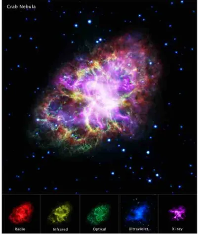
A famous example of a pulsar surrounded by its own nebula is the Crab Neb-ula (Figure 1.10), the remnant of a SN observed by Chinese astronomers in 1054 which has been emitting “-radiation of energy ¥ TeV for around 1000 years.

1.6.3 Active Galactic Nuclei

Active Galactic Nuclei (AGN) are galaxies with an unusual emission that is not associated with stars and produces a non-thermal component in the Spectral Energy Distribution (SED)5_{, in contrast to normal galaxies whose total luminosity is the}

sum of the thermal emission from each star. This difference from usual galaxies is due to the presence of a super massive black hole (SMBH) in their center, which is actively accreting matter from the surrounding environment. This allows them to

(19)

1.6 Sources of High Energy CRs and Hillas plot 15

Figure 1.10. Crab Nebula by five observatories: VLA/NRAO/AUI/NSF, Chandra/CXC,

Spitzer/JPL-Caltech, XMM-Newton/ESA, and Hubble/STScI. Credit: NASA https: //photojournal.jpl.nasa.gov/figures/PIA21474_fig1.jpg

reach extremely high luminosity values (¥ 1048 _{erg/s). Consider the accretion onto}

a black hole; the maximal energy gain is

Emax≥ GmM RS RS=2GM/c2 æ Emax= mc 2 2 (1.25)

where RS is the Schwarzschild radius6, G is the gravitational constant, M is the mass of the central BH, m is the accreting mass and c is the speed of light. A large part of this energy is lost in the black hole, while the remainder heats up via friction an accretion disc (optically thick disk of material) around the black hole. The luminosity from accretion is

L= ‘c 2_dm

2dt . (1.26)

By replacing standard values for the black hole activity (dm/dt = 1 M§/yr) and the accretion efficiency (‘ = 5% ≠ 42%, depending on the spin of the black hole [75]), high luminosities are obtained. There exist different types of AGN, illustrated in

6_{Radius of the event horizon surrounding a non-rotating black hole. Any object with a physical}

radius smaller than its Schwarzschild radius will be a black hole. This quantity was first derived by Karl Schwarzschild in 1916.

(20)

(a) (b)

Figure 1.11. Figure (a): The unified scheme of AGN. [79]. Figure (b): AGN classification

scheme. [56].

Figure 1.11, unified by the same phenomenon-accretion. The different characteristics, for example the fast variability of their spectra, is a consequence of different angles of view, different stages of activity and evolution in time. The most interesting active galaxies for us are Blazars, AGN with a relativistic jet pointed in the direction of the Earth, which makes them the most promising sources of ultrahigh energy cosmic rays. If the jet points directly towards the observer, the relativistic beaming effects make the source appear very luminous in the radio band and often extremely variable [56].

AGN have also considered very promising sources of high-energy neutrinos un-til now and this has been recently confirmed by IceCube, which found a coincidence in direction and time between an high-energy neutrino event detected on 22 Septem-ber 2017 and a gamma-ray flare from the blazar TXS 0506+056 [8]. This suggests that blazars are possible contributors to of the high-energy astrophysical neutrino flux. This discovery is very important because the detection or not of neutrino radiation from AGN or other astrophysical objects (e.g. GRBs) can provide unique information about the processes characterising of their central engine and the pres-ence of relativistic protons of sufficiently high energy in the relativistic jet (see Chapter 2 for the explanation of this topic, done in the the context of gamma-ray bursts but also valid for AGN).

1.6.4 Gamma-Ray Bursts

Gamma-Ray Bursts are the most luminous objects in the Universe and represent highly beamed sources of gamma-rays and perhaps also of high energy neutrinos and cosmic rays: in the internal shock scenario, blobs of plasma emitted from a central engine collide within a relativistic jet and form shocks, producing particle acceleration and neutrino emission. A distinctive feature is the high Lorentz factor of shocks in GRBs, which however poses severe challenges to the efficiency of shock acceleration in these extreme environments.

(21)

17

Chapter 2

Gamma-Ray Burst

Gamma-Ray Bursts (GRBs) are brief pulses of gamma-ray radiation as a consequence of the most powerful known explosions in the Universe. They were casually discovered by the U. S. Vela satellites1_{, built to detect the gamma radiation pulses emitted by}

nuclear weapons tested in the space.

The first unexpected signal was detected in 1967 and subsequently Klebesadel et al. (1973) [80] showed that Vela spacecraft observed sixteen short burst of photons in

the energy range 0.2 ≠ 1.5 MeV between 1969 July and 1972 July. Bursts duration ranged from less than 0.1 s to ≥ 30 s and time-integrated flux (also called fluence) from ≥ 10≠5 _{erg cm}≠2 _{to ≥ 2 ◊ 10}≠4 _{erg cm}≠2_{. Several count rate records were}

composed by a number of clearly resolved peaks, showing significant time structure within bursts, while other did not appear to display any significant structure.

Figure 2.1. Count rate as a function of time for the GRB of 1970 August 22 as recorded

by three Vela spacecrafts. Arrows indicate some of the common structures. Background count rates preceding the burst are also shown [80].

1_{Satellites launched by the United States starting from 1963 to monitor compliance with the}

treaty "banning nuclear weapon tests in the atmosphere, in outer space and under water" signed by the governments of the Soviet Union, the United Kingdom and the United States in 1963.

(22)

These bursts were not related in time or direction to any nova or supernova and it was demonstrated also that the energy observed was consistent with an extreme explosion as a source. It was also checked that these bursts were not coming from the Sun, Moon, or other planets in our solar system. Interestingly, the first evidence for the source at the origin of GRB is constituted by the simultaneous detection of gravitational waves in space and time correlation with the high-energy gamma-ray emission of a short GRB, namely GRB170817A [11]. For this class of GRB, namely where the duration of the emission is faster than 2 s, binary systems of colliding neutron stars are believed to be the progenitors of the emission. On the other hand, for long GRB (gamma-ray duration longer than 2 s), core-collapse SNe are considered the most plausible progenitor candidates.

2.1 Majors experiments and their results

BATSE: 1991-2000

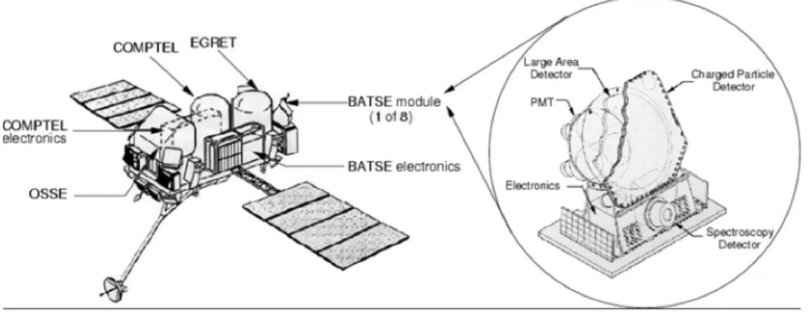
In 1991 GRB study really began, when the Compton Gamma-Ray Observatory (CGRO) was launched from space shuttle Atlantis in a low Earth orbit, at 450 km, to observe the high-energy Universe. It carried four different instruments, that provided a wide energy band coverage of 20 keV - 30 GeV: the Burst And Transient

Source Experiment (BATSE), the Oriented Scintillation Spectrometer Experiment

(OSSE), the Imaging Compton Telescope (COMPTEL) and the Energetic

Gamma-Ray Experiment Telescope (EGRET).

BATSE, in particular, was an important starting point for the study of GRBs; one of its primary objectives was the study of those phenomena at that time still mysterious, which are the gamma-ray bursts [55]. It was sensible in an energy range going from 20 keV to 10 MeV. Eight uncollimated detector modules were positioned around the spacecraft to provide an unobstructed view of the sky (see Figure 2.2). The plastic scintillator, a large-area detector, provided a high sensitivity for weak bursts and fine time structure studies for the stronger ones. A spectroscopy scintillation device was included in each detector module: it was optimized to obtain better energy resolution and to cover a wider energy range than the large-area detector.

Figure 2.2. The Compton Gamma Ray Observatory and one of the eight BATSE detector

(23)

2.1 Majors experiments and their results 19 BATSE was able to see the whole sky and detected about 1 GRB per day, identifying the extragalactic origin of GRBs as probed by the isotropic angular distribution of these events (see Figure 2.3) [99]. Thanks to an analysis of 153 gamma-ray bursts, a deficit on low luminosity (and thus in energy, too) GRBs was seen, indicating that they are either located in galaxy halos, or are from cosmological origin, in which case the deficit at low energy would be due to the expansion of the Universe.

Figure 2.3. Locations of the Gamma ray bursts detected by BATSE projected in galactic

coordinates (the Milky Way stretches horizontally across the centre of the figure). The colours indicate the energy and duration of each burst: long duration bright bursts appear in red while short duration weak bursts in purple. The grey points indicate bursts for which the energy and/or duration could not be calculated. Figure from https://gammaray.nsstc.nasa.gov/batse/grb/skymap/.

Furthermore, BATSE clearly saw two distinct populations of burst, short and long (for more details see Section 2.2.2) but, except for their duration, it did not find

other significant differences, due to the lack of additional data.

Beppo-SAX: 1996-2002

Beppo-SAX was an Italian satellite launched on April 30, 1996. It had on board

various X-ray detectors (to measure a radiation lower in energy than gamma) in addition to a GRB monitor. Therefore, it was the first X-ray mission with a scientific payload covering an energy range from 0.1 to 300 keV and with the ability to provide an angular position of bursts to within 4 arc-minutes (improved more than a factor 20 if compared to the CGRO) [87]. This allowed to observe for the first time the

afterglow, a rapidly fading X-ray emission associated with the GRB jet expansion

in the ISM. On February 28, 1997, Beppo-SAX saw a burst and, about a day after, an X-ray afterglow [48]. Ground-based spectrometers were able to measure also the optical spectrum of the afterglow.

The extragalactic origin of GRBs (cosmological distances, i.e. z ≥ 1) was unequivo-cally established three months later, when GRB 979508 was localized and its redshift was estimated (z ≥ 0.84) [96].

(24)

Thanks to Beppo-SAX, could also be estimated the energy involved in these phe-nomena. From the measured values of the burst redshift and of the flux, it was obtained that GRBs radiate 1048_{≠ 10}55 _{erg (if isotropic). This means that GRBs}

are the most energetic and explosive sources in the known Universe [86]. This opened a new era in the study of these objects with important questions:

• Can these distant objects exist with such a great flow? • What does cause them?

Swift: 2004-now

Swift Gamma Ray Burst Explorer, or simply Swift, was launched into a low-Earth

orbit on November 20, 2004 and is still operating. It is composed by three instruments working together to provide rapid identification of GRBs and to observe afterglows in the gamma-ray, X-ray, ultraviolet and optical wavebands [61]:

• Burst Alert Telescope (BAT): 15-150 keV

With its large field of view (2 sr) and high sensitivity, it detects about 100 GRBs per year and computes burst positions onboard the satellite with arc-minute positional accuracy.

• X-ray Telescope (XRT): 0.3-10 keV

It takes images and is able to obtain spectra of GRB afterglows during pointed follow-up observations.

• UV/Optical Telescope (UVOT): 170-600 nm

It takes images and can obtain spectra of GRB afterglows during pointed follow-up observations. It provides a position localization of about 0.5 arcsec and allows to track the temporal evolution of the UV/optical emission. The important discovery made by Swift is represented by the first localization of a short GRB with its afterglow, in that such an observation had never been performed before (GRB 050509B). Gehrels et al. (2005) [62] found that its position on the sky was near a luminous, non-star forming elliptical galaxy at redshift z = 0.225, exactly the type of location one would expect if the origin of this GRB is the merger of neutron star or black hole binaries. This, combined with correlations of long GRBs with supernovae, allowed to partially address the origin of these objects, after more than 30 years since their discovery.

Swift satellite has also found GRBs at very high redshift, until z = 9.4, when the Universe was just 0.52 billion years old [49]. Therefore, GRBs represent impor-tant probes of the end of cosmic dark age, when the first stars and galaxies were forming.

Fermi: 2008-now

The Fermi satellite, launched in June 2008 and still in operation, has been providing useful data measuring radiation in an energy window extending from ≥ 8 keV to

>300 GeV to help answer some open issues about GRBs: what phenomenon does

(25)

2.2 Observational properties of GRB prompt radiation 21

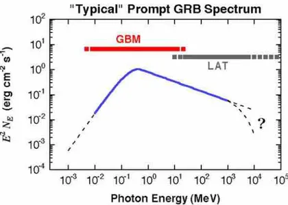
Figure 2.4. Band spectrum. In red and grey gamma-ray burst spectral coverage of the

GBM and the LAT, respectively, are indicated.

phenomena? How will the study of these energetic objects improve the understanding of the nature of the Universe and how it behaves?

This satellite is constituted by two instruments:

• Gamma-Ray Burst Monitor (GBM): 8 keV-40 MeV

It is dedicated to the study of GRBs by extending the LAT energy range over the full unocculted (by the Earth) sky. It uses an array of twelve sodium iodide scintillators and two bismuth germanate scintillators to detect gamma rays. GBM generates on-board triggers for ≥ 250 GRBs per years with a large field of view (≥ 8¶_{) [95].}

• Large Area Telescope (LAT): 20 MeV-300 GeV

It is able to detect the direction and energy of gamma rays with unheard-of resolution and sensitivity by using 880000 silicon microstrip detectors. It has a reduced field of view with respect to GBM, around 2 sr, allowing a better resolution in the reconstruction of direction (≥1 arcmin) [25].

The GBM-LAT combination thus provides burst spectra over seven decades in energy and has made several important discoveries regarding GRBs, in particular about their prompt spectra. In most cases they consist of one peak and power law functions with different indices at low and high energies with a smooth transition from one to the other (the so-called Band spectrum); in a few cases there is an additional non-thermal component that can be fit as a power law extending to high energies [128]. For more details see Section 2.2.1.

2.2 Observational properties of GRB prompt radiation

The prompt emission lasts typically a few seconds (or less), without repetition and with variable light curve. Furthermore, the spectra vary from burst to burst

(26)

and do not show any clear feature that could easily be associated with any simple emission model. Observationally, the prompt emission phase of a GRB is defined as a temporal phase during which sub-MeV emission is observed by GRBs detectors above the background level.

In this Section the basic features of GRB prompt emission will be treated.

2.2.1 Spectral properties

GRBs are characterized by emission in the few hundred keV range with a non-thermal spectrum, which can be fit with a smoothly-joined broken power law known as Band

function, introduced by Band et al. [29]: N(E) =

Y ] [

A1_{100 keV}E 2–exp(≠_EE₀), E <(– ≠ —)E0

AË(–≠—)E_{100 keV}0È–≠—exp(— ≠ –)1_{100 keV}E 2—, E_{Ø (– ≠ —)E}₀ , (2.1)

in which A is a normalization constant, N(E) is the number of photons detected, – and — (both negative) are the photon spectral indices below and above the break energy E0, respectively. The lower energy spectral index has generally a value –_{≥ ≠1, the high-energy one instead — ≥ ≠2. In the following, the flux particle F}‹ is referred to EN(E) while the SED to E2_N_{(E) or ‹F}

‹. For most observed values of – and — the SED peaks at Ep = (– + 2)E0, called E-peak, which represents the typical energy of the observed radiation. The Ep distribution is wide and extends from several keV to the MeV range. An example of Band-function spectrum is shown in Figure 2.5.

Figure 2.5. The Band function spectrum of GRB 990123. Ep = 720 ± 10 keV, – =

(27)

2.2 Observational properties of GRB prompt radiation 23 Some spectra can be fitted with a simpler function, a cutoff power law spectrum in the form: N(E) = A 3 _E 100 keV 4≠– exp3≠E Ec 4 , (2.2)

that is essentially the first portion of the Band function 2.1. In this expression Ec characterize the cut-off in the energy spectrum. This function has been used to fit the prompt spectrum of many GRBs (e.g. Fermi-GBM spectra [101]), mainly because of the narrow bandpass of the detectors, so that — could not be well constrained. When the spectrum is observed simultaneously by several instruments it is possible to obtain the global spectrum, and possibly it still comply with a Band function. However, GRB spectra measurements have evolved considerably from Band function in the years. Extra-components have been introduced: e.g. high-energy power law of exponentially attenuated power law [65] and photospheric component [110].

2.2.2 Temporal properties

The duration of a GRB is estimated through the so-called T90, the time interval

between the moment in which the 5% and the 95% of the fluence2 _{are released. It}

typically ranges from millisecond to thousands of seconds and allows to define two different GRB types [84]; in fact, the T90 distribution of GRBs detected by BATSE

on board CGRO, shown in Figure 2.6, includes two components with a separation visible around 2 s:

• Short-GRBs: burst duration peaked at 0.3 s, probably result of mergers of compact objects in binary systems (e.g two neutron stars or a neutron star and a black hole) [92].

• Long-GRBs: burst duration from ≥ 2 s to many minutes, peaked at 30 s. These are associated with massive stars collapsing and generating supernova explosions [92].

The GRB separation into two classes is related to the "hardness ratio", that is the ratio between the photon numbers in the detector’s low-energy and high-energy bands. Long GRBs in most of the cases have a "softer" spectrum than short ones, because in the first case the hardness ratio is larger than in the second one. However,

T90 has some limitations, because it is a quantity defined by observations:

• It is energy-band-dependent and sensitivity-dependent; a detector with a lower energy bandpass typically gets a longer T90 for the same GRB and a more

sensitive detector would detect a longer duration of a same burst along the background level.

• It can overestimate the duration of GRB central engine activity; it is the case of GRBs with clearly separated emission episodes with long quiescent gaps in between.

(28)

Figure 2.6. T90 distribution of the 4B Catalog Gamma-Ray Bursts recorded with BATSE. The result is a bimodal distribution, which reflects the existence of two GRBs population: long and short GRBs span T90durations greater and less than ≥ 2 s, respectively. Figure from https://gammaray.nsstc.nasa.gov/batse/grb/duration/.

Time scales - Observations

To date, there is a great variety of GRB light curves. Most of them are variable, while other are smooth with relatively simple temporal structures. One sample of GRB light curves is shown in Figure 2.7. By analyzing a light curve one can define two quantities:

• The variability time scale ”t, which is determined by the width of the peaks in a light curve. It can be of the order of milliseconds for extremely variable GRBs.

• The pulse separation t. When this quantity is large, the distance between the two neighboring peaks is classified as a quiescent period, a relatively long period of several dozen of seconds with no activity.

Both their distributions follow log-normal ones (see e.g. [100]). By studying ”t and

t distributions one can obtain important information about the central engine

activity; this topic will be better discussed in Chapter 4.

The considerations made up to now are valid for long GRBs; the variability of short ones is more difficult to analyze. Indeed, the duration of these bursts is closer to the limiting temporal resolution of the detectors.

Time scales - Theory

General kinematic considerations impose constraints on the temporal structure produced when the energy of a relativistic shell is converted to radiation [105].

(29)

2.2 Observational properties of GRB prompt radiation 25

Figure 2.7. Examples of GRB light curves detected by BATSE. Figure from [103]. Consider a spherical relativistic emitting shell with a radius Re, a width and a Lorentz factor “ © , referring to the Figure 2.8. Photons emitted in point A move directly towards the observer and arrive first after a time trad; if they are emitted

moving at an angle ≠1 _{(point D) they will arrive after t}_ang_{= R}

e/2c 2 3. This time might possibly coincide with the arrival time of photons emitted in point C, directly towards the observer but at a radius 2Re. So, in this case, tang¥ trad. This suggests that variable GRBs cannot be produced from a single explosion. Other time scales are determined by the flow of relativistic particles. First of all, the intrinsic duration

T = /c, which is the time in which the source that produces the relativistic flow

is active; photons emitted at the front of a such shell will reach the observer at time

T before those emitted from the rear (point B). Secondly there is the intrinsic

variability ”t , which is the time scale on which the inner source varies and produces a subsequent variability with a lenght scale ” = c”t in the flow. Naturally ”t sets a lower limit to the variability time scale observed in any burst.

These timescales divide light curves into two classes:

• T Æ tang ¥ trad: the resulting burst is smooth with a width tang¥ trad. This

is the case of external shocks, i.e. when shells interact with the interstellar medium [111], then external shocks can produce only smooth bursts.

• T > tang: a variable light curve is producted. This can be easily satisfied in

the internal shock model (see Section 2.3.1).

(30)

Figure 2.8. Different time scales from a relativistic expanding shell in terms of the arrival

times of various photons: the angular time scale tang= tD≠ tA, the radial time scale

trad= tC≠ tA and the intrinsic duration of the flow T = tB≠ tA. Figure from [105].

2.3 GRB fireball model

The so-called fireball model is the basic model proposed to explain the first ob-servations of GRBs [66] [102]. It consists into a matter-dominated fireball, made of baryons (primarily protons and neutrons), electron-positron (e+_e≠_{) pairs, and}

photons, created after the collapse of massive stars (long GRBs) or after the merging of binary objects (short GRBs).

Figure 2.9. Cartoon for the GRB fireball model. Figure from [63].

As shown in Figure 2.9, a high amount of energy is released by the central engine and a relativistic outflow is formed by parts of this energy. This outflow is accelerated and part of its kinetic energy is dissipated through the prompt emission mechanism (generated by internal shocks between slow and fast parts of the ejecta), leading to

the observed “-ray emission.

The sudden release of a large amount of “-ray photons leads via e+_e≠ _{pair creation}

to an opaque radiation plasma. The energy in radiation is initially larger than in baryons by a factor of about 102_{, and as the fireball expands adiabatically, baryons}

get accelerated to a high Lorentz factor, then to relativistic velocities [112]. The kinetic energy of the outflow is converted back to thermal energy and radiated

(31)

2.3 GRB fireball model 27 away as “-rays photons at some large distances from the place where the fireball is produced (e.g. [107]). When the baryon kinetic energy becomes comparable to the total fireball energy, the acceleration stops. The matter-dominated fireball continue to expand and becomes more and more transparent to radiation, so the jet now is optically thin. In this phase, parts of the kinetic energy are dissipated by the prompt emission and the subsequent radiation is detected as the non-thermal prompt emission. When the created jet reaches the circumburst medium external shocks create the afterglow and the jet is finally decelerated. The remaining kinetic energy powers the observed multiwavelenght afterglow.

However, the exact energy dissipation and emission mechanism is still under debate and is closely connected to the nature of the ejecta itself.

The compactness problem and relativistic motion

Now it is known that the GRB central engine emits ultra-relativistic jets but at the beginning of GRB studies it was not trivial to understand it. The relativistic motion in these objects, in fact, was rising the so-called compactness problem.

The optical depth of the process “ + “ æ e+_e≠ _{is given by ·}

““ Ã L/R, where L is the luminosity and R the size of the emitting region. A simple estimate of the size of the source (R = c”t, as implied by the observed variability, where ”t is of the order of milliseconds) shows that the source must be extremely optically thick to e+_e≠ _{pair creation. Such a source cannot provide the observed non-thermal}

gamma-ray emission. The solution of this paradox is hidden in the relativistic motion for two reasons:

1. The size of the emitting region becomes now R = c 2_”t_{, where is the average}

Lorentz factor of the jet.

2. The rest frame energy of the photons is smaller by a factor of ; therefore, only a smaller fraction of them can create pairs.

If > 100, the pair creation optical depth would be reduced below 1 and high-energy photons would be able to escape the fireball.

The potential of relativistic motion to resolve the compactness problem was re-alized, among other scientists, in the eighties by Goodman [67] and Pacz˝nski [102].

2.3.1 GRB prompt emission models

Internal Shock Toy Model

A widely used model to describe the activity of the inner engine is the so-called

internal shocks model (IS). In this scenario, the source produces multiple shells

with different Lorentz factors over a time T = /c, where is now the overall width of the flow in the observer frame (see Figure 2.10). Faster shells will catch up with slower ones and will collide, converting some of their kinetic energy to internal

(32)

Figure 2.10. The internal shock model. Figure from [105].

energy [103]. The source is variable on a scale L/c, where L is the distance between two adjacent shells, then the observed variability time scale in the light curve, ”t, reflects the variability of the source. The characteristic radius where the shell starts to collide is Rcoll ¥ L 2 and continue as long as the source is active, within the

duration time T , reflecting the overall duration of the activity of the inner engine. In the following, the shell collision process is considered. For semplicity, we assume two shells of masses m1 and m2 ejected from the central engine with Lorentz factors 1 and 2, respectively. The slower shell is launched from the source ”t time before

a faster shell. When the latter reaches the first one, they collide forming one single shell distant from the center Rcoll ¥ 2c 21”t, when 2 & 2 1. Therefore, the radiation

produced in this collision arrives at the observer at time:

tobs≥ t0+_2cRcoll₂

f

≥ t0+ ”t 1

2, (2.3)

where t0 is the time when the faster shell was ejected from the central engine, f is the final Lorentz factor of merged shells, given by:

f =

m_{1 1}+ m_{2 2}

(m2

1+ m22+ 2m1m2 r)1/2, (2.4)

where r is the relative Lorentz factor of the two shells before collision. From Equation 2.3 it is clear that the variability time of GRB light curves roughly tracks the engine variability time (assuming that 2/ 1 does not change during the engine

activity). Therefore, the internal shocks model can explain the observed short time scale variability by linking it to the central engine time scale.

In the internal shock scenario it is expected that particle acceleration happens at the shock created in the collisions between shells. The radiation emitted by accelerated particles forms the prompt non-thermal spectrum, which is generally

(33)

2.3 GRB fireball model 29 explained by the synchrotron emission4 _{or by Inverse Compton (IC)}5_.

The internal shock model, however, does not dissipate efficiently the shock kinetic energy, because of the intrinsic relativistic nature of the shock itself. In fact, defining the efficiency as the total GRB energy divided by the radiated energy (also including the afterglow) one would expect an high efficiency (Ø 50%) [78]. Only a fraction of the thermal energy produced in collisions is likely deposited in electrons, the rest is taken up by protons and magnetic fields [87] and the synchrotron and the IC power losses for a proton are smaller than for an electron. A high efficiency in “-rays production requires a large dispersion in the Lorentz factor of the outflows [31], that in turn makes difficult to accomodate some observed spectral relations [78].

Photospheric model

The photospheric model (PH) is often address to explain thermal photons observed in GRB spectra. While in the internal shock model all radiation emission is produced in the optically thin regime, the photospheric scenario assumes the emission to be released at the photosphere itself. However, the spectrum that it produces tends to be thermal without non-thermal tails observed in GRBs [78]. It is reasonable to think that in GRBs both models coexist, also because, assuming that the photospheric model is the only valid, one would not be able to observe “-rays; the radiation, in fact, would be released in a region where the flow is optically thick, hence photons would not escape the fireball.

Figure 2.11. Photospheric-internal-external shock model. The photospheric emission

produces the Band spectrum, the internal shock contributes to the variable power law spectrum, and the external shock makes the long-lived power law spectrum. Figure from [78].

This scenario can explain sub-dominant thermal features measured for some burst detected by Fermi satellite [118].

4_{Non-thermal radiation generated by charged particles (usually electrons) spiralling around}

magnetic field lines at close to the speed of light. Since the electrons are always changing direction, they are in effect accelerating and emitting photons with frequencies determined by the speed of the electron at that instant.

5 _{Scattering of low energy photons to high energies by ultrarelativistic electrons so that the}

(34)

In Figure 2.11 the photospheric-internal-external shock model and corresponding energies affected in the radiation spectrum are shown. See the recent review [32] for new developments of this model.

2.4 High energy neutrinos from GRBs

Both the internal shock and the photospheric models assume that shocks take place when faster shells of plasma emitted by the central engine collide with the slower ones, producing gamma rays. This mechanism dissipates a large fraction of the kinetic energy of the flow, provided that the central engine is highly variable. The dissipated energy is partly transferred to accelerated particles, namely electrons and protons, which then assume ultra-relativistic speed. At this point accelerated electrons radiate a fraction of their energy through synchrotron and inverse Compton processes, creating a radiation field that possibly allows the p“ resonant + _{production, and}

the subsequent decay chain:

p+ “ æ+ I p+ fi0 n+ fi+ æ Y _ _ _ _ _ ] _ _ _ _ _ [ fi0 æ “ + “ n_{æ p + e}≠+ ¯‹e fi+ æ µ++ ‹µ µ+ _{æ e}++ ‹e+ ¯‹µ (2.5) Protons of energy Ep ≥ 1015 eV interact with keV-MeV photons forming + res-onance (m + = 1232 MeV/c2) which decays into pions, forming neutrinos with

E‹ ≥ 1014 eV. Therefore, assuming that the proton load (the fraction of protons in the flux of accelerated particles) is not negligible, GRBs are believed to be im-portant high-energy neutrino producers. About 20% of the proton energy goes to

fi+ (E_fi+ ≥ 0.2E_p), whose energy is evenly distributed to 4 leptons (E_‹ ≥ 0.25E_fi+);

so overall E‹ ≥ 0.05Ep [87]. Due to the high compactness of the ejecta, the p“ interaction can have high optical depth, so that ﬁ+ _{are copiously generated. These}

latter decay in µ+_{, which subsequently decay generating neutrinos (‹}

µ and ‹e) and anti-neutrinos ( ¯‹µ).

The mechanism indicated in 2.5 can take place in both the PH and IS models, but the difference lies in the distance from the central engine in which the main collision occurs, as it affects the energies involved in the collision. The standard model invokes internal shocks as the site of both “-ray photon emission and proton acceleration; alternatively, in the photospheric model photons can be generated at the photosphere and protons can be accelerated in the same site [87]. Therefore, in this latter case the emitted neutrino energy will be lower than that in the internal shock model; the emission of neutrinos, in fact, takes place before the particles undergo further acceleration from the collision between different shock fronts. In fact, the neutrino production efficiency is different in the two cases. The optical depth ·p“ of p“ interaction is [121] [126]: ·p“= 0.8 3 _R 1014_cm 4≠13 102.5 4≠23 _E “ 1 MeV 4≠13 _L_iso 1052_{erg s}≠1 4 , (2.6)

where R is the distance between the central engine and the neutrino production site (fireball radius), Liso is the isotropic “-ray luminosity of the burst and E“ is the

(35)

2.4 High energy neutrinos from GRBs 31 energy at which the “-ray spectrum has a break (≥ 100 keV). In the IS scenario R depends on the variability time tvar, the Lorentz factor and the redshift z, and it

is given by [27]: RIS≥ 1013 3 _t var 0.01 s 4 3 102.5 423_{1 + 2.15} 1 + z 4 cm, (2.7)

while in the PH scenario is [127]:

RPH≥ 1011 3 102.5 4≠23 _L_iso 1052_{erg s}≠1 4 cm. (2.8)

For characteristic values of GRB parameters RPH< RIS, then ·p“ in the PH model is enhanced by a factor RIS/RPH compared to the IS model. This result suggests

that the neutrino production is more efficient in a dissipative photosphere than in standard ISs [20].

In hadronic GRB models, neutrinos are produced from the interaction between the accelerated protons and the jet radiation field. Accelerated protons are expected to be distributed according to a differential energy spectrum in the form indicated by Equation 1.8 with (1 + s) = 2. Convolving such a spectrum with the spectrum of the target radiation field, one generally expects for the neutrino energy distribution a power law spectrum with an energy break regulated by the break in the synchrotron spectrum of target photons. The first calculation of the prompt neutrino flux was realized by Waxman & Bahcall (1997) [121], which used average GRB parameters and the GRB rate measured by BATSE to determine an all-sky diffuse neutrino flux contributed by the GRB population. In this work another general formalism that can be applied to any of the above mentioned models for GRB emission is presented. It was calculated by Abbasi et al. (2010) [10], following Guetta et al. (2014) [69], which is in turn based on Waxman & Bahcall (1997) [121]. For an observed "Band" function photon flux spectrum

F“(E“) = dN(E_dE “) “ = f“ Y _ ] _ [ ! ‘“ MeV"– 1 _E “ MeV 2≠– , E“< ‘“ ! ‘“ MeV"— 1 _E “ MeV 2≠— , E“ Ø ‘“ (2.9) where ‘“ is the break energy, – and — are the spectra index before and after the break energy, respectively, and f“ is the normalization, the observed neutrino number spectrum can be expressed as:

F‹(E‹) = dN(E_dE ‹) ‹ = f‹ Y _ _ _ _ ] _ _ _ _ [ !‘‹,1 GeV"–‹ 1 E‹ GeV 2_≠–‹ , !‘‹,1 GeV"—‹ 1 E‹ GeV 2≠—‹ , !‘‹,1 GeV"—‹!GeV‘‹,2"“‹≠—‹ 1 E‹ GeV 2≠“‹ , E‹ < ‘‹,1 ‘‹,1Æ E‹ < ‘‹,2 E‹ Ø ‘‹,2 (2.10) where –‹ = p + 1 ≠ —, —‹ = p + 1 ≠ –‹ and “‹ = —‹ + 2; p = 1 + s is the photon spectral index defined by N(Ep)dEp Ã Ep≠pdEp. The indices –‹ and —‹ are derived by assuming that the neutrino flux is proportional to the p“ optical depth ·p“. This is valid when the fraction of proton energy that goes to pion production is proportional