EXPERIMENTAL DATA COLLECTION AND MODELLING OF DRY DEPOSITION VELOCITIES FOR URBAN SURFACES 1. PARTICLES DRY DEPOSITION PROCESSES
1.1 Introduction
Dry deposition process is one of the important pathways for the removal of radioactive particles from atmosphere. It is the result of a combination of different environmental and physical factors as atmospheric conditions, particle properties, characteristics of the canopy. For this latter factor, the urban canopy represents unevenly combinations of different types of surface elements that increases the complexity of the involved phenomena that influence particle depositions.
Smooth surfaces tend to have lower deposition rates per unit area than rougher surfaces. Such relatively small deposition rates are reported by Roed (1983) for Cs137 surface deposition, on vertical walls, in Denmark. The paper reports the results of nine samples for a brick wall with a range of wet/dry deposition velocities 0.003 to 0.07 cm/s, four samples for a plastered wall with a range of 0.014 to 0.085 cm/s, and only one sample is in an area sheltered from wet deposition and had a dry deposition velocity of 0.003 cm/s.
Nicholson (1987) reported similarly small deposition rates for deposition of Cs134 and Cs137 particles to roof and building materials in England. Although the data set was small, the results were consistent with lower deposition velocities over smoother surfaces.
In (Papastefanou, 2008) an up-to-date summary of knowledge about depositions of radioactive aerosols is provided. The experimental deposition velocities reported in Tab. 1.1 highlighted that for Be7 particles varied from 0.1 to 3.4 cm/s, for Pb210 from 0.7 to 1.1 cm/s and for Cs137 from 1.3 to 6.3 cm/s. These data refer mostly to temperate latitudes of the Northern Hemisphere, e.g. at Thessaloniki, Greece 40°N, Oak Ridge, TN 36°N (Mahoney, 1984), Norfolk, VA 37°N (Todd et al., 1989), New Haven, CT 41°N (Turekian et al., 1983), Detroit, MI 42°N (McNeary and Baskaran, 2003), Qulllauyte, WA 49°N (Crecelius, 1981), Munich, Germany 49°N (Rosner et al., 1996).
Table 1.1 Deposition velocity of atmospheric particles, Vd (cm/s)
7Be 210Pb 137Cs Investigation Country
0.5 (0.3–0.8) – 3.4 (1.3–6.3) Papastefanou et al. (1995) Greece
1.2 (0.5–2.1) – – Chamberlain (1953) UK
0.80 – Young and Silker (1980) USA
1.0 – – Crecelius (1981) USA
2.8 0.95 – Turekian et al. (1983) USA
1.66 – – Mahoney (1984) USA
1.3 0.7 – Todd et al. (1989) USA
1.5 – 1.46 Rosner et al. (1996) Germany
1.6 1.1 – McNeary and Baskaran (2003) USA
The approach for determining deposition rates has several limitations for urban area. Considering the total deposition per unit horizontal area, grass and trees have relatively high deposition rates compared to smooth surfaces. Considerable variability in deposition rates occurs because of the variability of exposures of surface elements to local air circulation. Moreover, the more contaminated air that flows over a surface per unit time, the greater will be deposition rate.
Analogous to the enhanced deposition on leeward sides of hills and waves, the leeward sides of urban structures tend to have higher deposition rates.
Some studies highlight that deposition is mainly controlled by large particles. By observing deposited particles, Tai et al. (1999) show that this effect is particularly true for urban locations where the coarse concentration of particles is high; however, the effect is also true for non-urban locations where the coarse concentration of particles is low. Similar results were obtained by Lee et al. (1996) for PCB (polychlorinated biphenyl) dry deposition in an urban area. Studies of urban deposition rates of hydrocarbons and metals show deposition-rate variations over urban areas that largely reflect the influence of local sources on ambient airborne contaminant concentrations (Azimi et al., 2005). Characterization of variations in the ambient aerosol size distribution, that typically occur across an urban area, complicates the modeling of in-plume aerosol interactions and, consequently, the computation of deposition rates.
It follows that the modelling of dry deposition phenomena within urban canopies is not easy to configure and, although empirical or semi-empirical models have been developed to address this complex aspect, there is not standardized and common accepted criteria proposed in literature (Droppo, 2006). Indeed, their application remains valid for specific conditions and if the data in that application meet all of the assumptions required by the data used to define the models.
1.2 The main phenomena in dry deposition processes
In atmospheric models, the Surface Layer (SL) is the air layer over the surface whose properties are largely controlled by the local surface fluxes (Fig. 1.1). The strict definition of the surface layer is a fully turbulent layer over homogenous surfaces under steady-state conditions.
With this surface layer, a second layer is designated that refers to the laminar, or near-laminar, flow that occurs immediately over the surfaces. This layer, which is referred to here as the “quasi-laminar layer”, may exist only intermittently in nature as the flow changes over the surfaces. In the literature, this layer is also referred to as the “laminar sublayer,” “sublayer,” or “deposition layer.”
Therefore, the main transport processes are:
transport due to atmospheric turbulence in the lower layer of the Planetary Boundary Layer (PBL), i.e. SL. This process is independent of the physical and chemical nature of the pollutant and it depends only on the turbulence level;
diffusion in the thin layer of air which overlooks the air-ground interface (i.e. quasi-laminar sublayer), where the dominant component becomes molecular diffusion for gasses, Brownian motion for particles and gravity for heavier particles;
transfer to the ground that exhibits a pronounced dependence on surface type with which the pollutant interacts (i.e. urban context, grass, forest, etc.).
On the basis of layer classifications, dry deposition phenomena involve three sequential sets of processes:
1. through the turbulent surface layer, the particle moves by the combined effects of eddy diffusion (i.e., carried by turbulent movements of air) and gravity.
2. in quasi-laminar surface layer, the particle can reach the surface by molecular diffusion, interception, or impaction.
3. near the surface, retention or rebound depends on a combination of surface and impact properties.
It is worth to note that the deposition process changes quite a lot over the year, for example due to the seasonal variation of vegetation (with or without leaf) or over the day in connection with meteorological conditions (e.g. influence of temperature on leaf stoma).
1.2.1 Eddy diffusion
Eddy diffusion refers to the transport resulting from turbulent movements in the air that play a pivotal role in determining the vertical transfer of momentum, heat and mass in the Atmospheric Boundary Layer (ABL) that usually encompasses the lowest tens to hundreds of meters in the atmosphere over the earth's surface (Garratt, 1992).
It is actively studied in boundary-layer meteorological modeling, however its impact on dry deposition in the modeling of atmospheric chemistry is not well characterized.
In approximately the lowest 10% of the ABL, i.e. the surface SL, the vertical fluxes of transferred quantities are nearly constant with height and can be represented quite successfully by formulations based on the Monin-Obukhov (M-O) similarity theory (Stull, 1988; H gstr m, 1988, 1996; Foken, 2006).
Under the assumption of steady state between generation, dissipation and transport of the turbulent eddies across the SL above the interfacial sublayer adjacent to surface obstacles, the M-O similarity theory describes relationships between vertical profiles and fluxes for momentum and scalar quantities (i.e., heat and trace constituents), using a metric called the Obukhov length L (Garratt, 1992):
(1.1)
in which is the average temperature in the SL (K); air density (g/cm3); c
p: specific heat at constant pressure [J/kg K]; g gravitational constant (cm/s2); H sensible heat (W/m2); k von Karman constant set at 0.4 [–].
The assumption of steady state provides a great advantage to the modeling of the surface fluxes, as the flux calculation requires the information of state variables only at two levels in this “constant-flux” layer within the SL. This allows to determine easily some relationships between the profile of wind speed and ABL meteorological conditions, as described in the following section.
Figure 1.1 - Air structure near the Earth’s Surface 1.2.1.1 Wind speed profile
Under the assumption of continued validity of the M-O flux-gradient relationships down into the interfacial sublayer, it is possible to evaluate wind speed profile as follows:
(1.2) with u(z) wind speed at deposition reference height (m/s); u* friction velocity, (m/s); k von Karman constant; z deposition reference height (m); zo surface roughness length (m); is the integrated stability-correction term for the wind profile.
To calculate the stability function in Eq. (1.2), Brandt et al. (2002) suggested the following relationship:
with > 0 (stable conditions) (1.3)
with < 0 (unstable conditions) (1.4) Under neutral atmospheric stability, Eq. (1.2) can be simplified as:
(1.5) The friction velocity parameter provides a measure of the intensity of atmospheric turbulence. For an aerodynamically rough but relatively flat surface, an extrapolation of the mean wind speed profile downward shows that it reaches zero at some distance above the physical surface. The height at which this occurs is called the roughness height (or roughness length), zo.
The roughness height is positively correlated with the physical roughness of the surface although a strict functional relationship between measures of physical roughness and zo do not exist. Some studies have found that the surface roughness length tends to be about one-tenth of the dimensions of the surface elements.
In environments with vegetation, such as over agricultural crops and forest canopies, the practice is to displace the entire velocity profile upward such that the height at which velocity profiles reach zero is the sum of a canopy roughness length, zo, and displacement height, d, which is defined as zero plane displacement (Fig. 1.2).
Fig. 1.3 reports a generalized mean wind velocity profile in a developed urban area and the zero-plane displacement length, d, for this configuration.
Consequently, Eq. (1.5) is modified as follows:
(1.6)
A simple scheme of distinct urban forms and roughness class, as reported in (Davenport et al., 2000), is illustrated in Table 1.2.
Table 1.3 reports for each roughness class the corresponding roughness length, zo. 1.2.2 Molecular diffusion
As above said, molecular diffusion by Brownian motion is usually assumed to dominate the diffusion processes in the quasi-laminar surface layer. However, there is the possibility that phoretic forces also can locally influence dry deposition fluxes.
Particles in the range of 0.001 to 0.1 (µm) (ultrafine particles) move like gaseous molecules in flowing air (i.e., they exhibit rapid random Brownian motion). Their motion causes them to collide with any nearby surfaces. Ultrafine particles tend to adhere to these surfaces as the result of intermolecular forces. This mechanism tends to be an effective deposition process with very small particles depositing at rapid rates on the nearest available surfaces.
Under some circumstances, this diffusion mechanism can continue to be the dominant deposition process for particles >0.1 µm.
Figure 1.3 - Generalized mean wind velocity, U, profile in a developed urban area. The heights are the mean height of the roughness elements (zH), the roughness length (z0) and zero-plane
Table 1.2 - Davenport classification of effective terrain roughness.
Urban Zone Image Roughness
class1
1. Intensely developed urban with detached close-set high-rise buildings with cladding, e.g. downtown towers
8
2. Intensely developed high density urban with 2–5 storey, attached or very close-set buildings often of brick or stone, e.g. old city core
7
3. Highly developed, medium density urban with row or detached but close-set houses, stores and apartments e.g. urban housing
7
4. Highly developed, low or medium density urban with large low buildings and paved parking, e.g. shopping mall, warehouses
5
5. Medium development, low density suburban with 1 or 2 storey houses, e.g. suburban housing
6
6. Mixed use with large buildings in open landscape, e.g. institutions such as hospital, university, airport
5
7. Semi-rural development, scattered houses in natural or agricultural area, e.g. farms, estates
4
1 Effective terrain roughness according to the Davenport classification (Davenport et al., 2000); see Table 1.3.
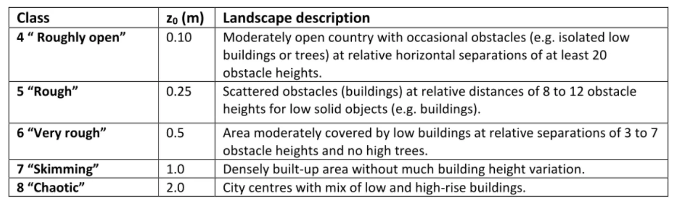
Table 1.3 - Davenport classification of effective terrain roughness Class z0 (m) Landscape description
4 “ Roughly open” 0.10 Moderately open country with occasional obstacles (e.g. isolated low buildings or trees) at relative horizontal separations of at least 20 obstacle heights.
5 “Rough” 0.25 Scattered obstacles (buildings) at relative distances of 8 to 12 obstacle heights for low solid objects (e.g. buildings).
6 “Very rough” 0.5 Area moderately covered by low buildings at relative separations of 3 to 7 obstacle heights and no high trees.
7 “Skimming” 1.0 Densely built-up area without much building height variation. 8 “Chaotic” 2.0 City centres with mix of low and high-rise buildings.
1.2.3 Phoretic Process
Electrostatic attraction causes the movement of charged particles in the presence of an electric field. The direction of movement depends on the direction of the field and the sign of the charge on the particle.
Attractive electrical forces have the potential to assist the transport of small particles through the quasi-laminar deposition layer and, thus, could increase the deposition velocity in situations with high local field strengths. However this effect is likely to be small in most natural circumstances (Hicks et al., 1982).
Diffusiophoresis can change the rate of dry deposition of particles embedded in a surface gradient of a gas, created by a condensation or evaporation of the gas to/from the surface. There is a difference in the kinetic energies imparted by collisions with up gradient and down gradient gas molecules. This process imparts momentum to the particles, which tends to move them down gradient for denser air gases and up gradient for lighter air gases. In addition, the introduction of new water vapor molecules at an evaporating surface displaces a certain volume of air. This effect, called Stefan flow, tends to reduce deposition flux from an evaporating surface.
Thermophoresis results in a net directional particle transport in the presence of a thermal gradient. For a particle in a thermal gradient, the air molecules striking one side of the particle will be more energetic than those on the other side. This effect will tend to move small particles away from a heated surface and towards a cooled surface.
In atmospheric dispersion models, phoretic on dry deposition are generally assumed to be small, based on their normally very small contributions to overall deposition fluxes (Hicks 1982). However, for particles in the range of 0.1÷1.0 µm, for which other deposition processes are relatively ineffective, these effects may not always be negligible.
Rather than including detailed formulations, dry deposition models generally include an empirical minimum limit for the magnitudes of deposition velocities. For example, the ISC Industrial Source Complex Model formulation (USEPA, 1994) adds a phoretic term to the deposition velocity modeled from diffusion, impaction, and gravitational settling; a constant value of 0.01 cm/s is added to the otherwise modeled deposition velocity to represent combined phoretic effects.
1.2.4 Gravitational settling
Gravitational settling is the downward motion of particles that results from the gravitational attraction. It is the dominant process for the dry deposition of the larger particles >10 µm.
Particulate sizes, densities, and shapes largely define gravitational settling rates.
The settling velocity for particles, vs, in (cm/s) can be computed using a modified form of Stokes Law (Hanna et al., 1982):
(1.7)
where ρp is the particle density, (g/cm3); μa the air dynamic viscosity (g/cm s); rp the particle radius, (cm); and Cc the Cunningham factor (-) expressed as (Seinfeld and Pandis, 1998):
(1.8) where λa is the mean free path of air (cm).
Non-spherical particles fall at slower rates. For materials with equivalent densities, the change in settling velocities is less than 30% for ellipsoid and cylinder shapes.
Engineering handbooks are also available with formulations for accounting for non-spherical effects. To account for shape effects, an aerodynamically equivalent diameter is frequently used to define the settling velocity of a particle.
1.2.5 Interception
The predominant deposition mechanism for particles in the range of 0.2 to 2 µm diameter is often assumed to be interception.
The large particles tend to move with the airflow streamlines, but too close to the obstacle so that it is captured on the surface.
Interception occurs most effectively when the surface element structures that the air is flowing through are smaller than the aerosol or solid particle diameter.
1.2.6 Impaction
Particles with diameters 2 µm and larger are effectively deposited by direct impact. These particles have sufficient momentum such that the particles do not follow the streamlines due to their inertia, resulting in the collision with the obstacle.
1.3 Reflections about particles aerodynamic diameter
Formulations for modeling dry deposition phenomena, can be significantly improved by expanding them to address the following ranges of particles potentially associated with an event:
very small particles (<0.05 µm). Molecular diffusion processes are dominant. Formulations for characterizing fluxes of these particles are normally based on Brownian motion. Although deposition from molecular diffusion processes is relatively well understood, the specific roles of thermal flux, concurrent mass fluxes, and electrical attraction are largely undefined. In an event, the very small particles will deposit quite rapidly either to the nearby surfaces or other particles in the plume. Because of the short time-scale, these deposition rates are normally not considered in air dispersion models but rather modeled as part of the plume initialization.
Small particles (0.05 ÷1 µm). This range includes the accumulation mode. The currently deployed dry deposition models provide surface-specific deposition estimates that agree relatively well with data from field and wind tunnel experiments. Stokes Law can be used to compute settling velocities. Implementation should include shape and size corrections to the Stokes equation. Although the Cunningham factor for the smaller particles tends to provide corrections to relatively small settling velocities, these corrections can potentially be important for defining the minimum deposition velocity for the accumulation mode.
Intermediate particles (1÷10 µm). Formulations for particle deposition need to address the range of situations from large surface elements with slow diffusion-driven rates to surfaces with a fine structure with faster impaction/interception driven rates. Current formulations that consider a combination of diffusion, impaction, and gravitational settling for specific types of applications should be incorporated into models to improve the estimates of deposition rates to the specific surfaces.
Larger particles (>10 µm). New formulations are available for significantly improving dry deposition computations for this range of particles. These improved formulations account for the importance of eddy inertial deposition efficiency in the deposition of these particles. Based on recent literature, older formulations, which are deployed in many models, are significantly under-predicting dry deposition rates for particles in this size range.
Very large particles (having sufficiently large size and density such that settling velocity >100 cm/s). Air dispersion models should incorporate particle trajectory-based modules accounting for reduced influences of atmospheric turbulence. This update represents a significant improvement for models that assume that all particles in the release are dispersed at the same rate.
2. URBAN DEPOSITION MODELS 2.1 Introduction
An urban area represents a complex area for assessment of potential exposures from an atmospheric release. A review of dry (and wet) deposition computational methods was conducted for radioactively contaminated particles (in the range 0.1 to 10 micron) by the Atmospheric Dispersion Modeling Liaison Committee (NRPB, 2001). They are recommend values and methods for estimating deposition rates and special parameter limits for extrapolation of the dry deposition model to an urban environment. However, neither of these reviews addressed the issues of the applicability of the dry deposition models to non-ideal conditions such as the aerodynamically very rough surfaces encountered in an urban environment.
Resistance-based approaches are widely used as a basis for dry deposition formulations. This approach, explained in more detail below, has the advantage of providing a means of combining a number of the processes controlling dry deposition into a single formulation.
In one of the early implementations, Sehmel and Hodgson (1978) proposed an empirical model based on curve fits to wind tunnel deposition results for a range of soil surface covers. Their model combined empirical data with the theory for molecular diffusion of very small particles and gravitational settling rates for larger particles.
The Authors also demonstrated the importance of considering the density of the particles in the dry deposition computation. Subsequent applications have included air quality (e.g., chemicals and trace metals), health physics (radionuclides), and acid rain models.
Detailed models, that address the processes leading to exposures in an urban environment, have been developed for radiological exposures (Jones et al., 2006).
Eged et al. (2006) used a Monte Carlo approach to evaluate potential radiological doses in urban environments. The results show that these urban dose computation models provide some results that are the same and some that are not.
To address the modeling of dry deposition in urban areas, some authors suggest an extension of the resistance-based formulations. For example, the NRPB (2001) review of dry deposition velocity estimation techniques for particles with a diameter of 0.1 to 10 microns suggests modifying the relationship for aerodynamic resistance for applications to higher canopies.
2.2 Resistance approach to describe dry deposition process
In mechanistic or process-based dry deposition models, an electrical resistance-based approach is widely used to parameterize the dry deposition velocity (Venkatram and Pleim, 1999).
By considering that the reciprocal of the dry deposition velocity, vd, is the overall resistance to the mass transfer, the influence of the various phenomena on the deposition velocity are expressed in terms of an electrical analogy.
The resistance approach evaluates a total resistance rt (s/cm) using the pollutant vertical flux F (g/cm2s) and the pollutant concentration C (g/cm3) at a reference height over the surface:
(2.1) where C0 is the concentration at the surface.
The condition for C0 to be close to zero occurs when all the material reaching the surface remains on itself (C0<< C), so the above formulation is:
On the basis of analogy with electrical circuits, the resistance to the mass transfer is configured as resistances in parallel and series circuits to describe transfer factor between air and surface.
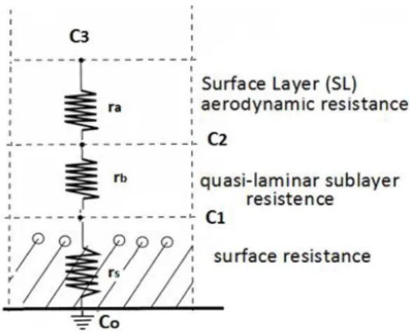
The dry deposition resistance for gas is considered as series circuits (Fig.2.1) that allows to write the following relationships:
(2.3)
where C1, C2, and C3 are concentrations at the layer boundaries such that C3 and C2 are concentrations across the turbulent surface layer, C2 and C1 are across the quasi-laminar surface layer, and eventually C1 and C0 shall identify the surface resistance.
In Eq. (2.3) ra is the aerodynamic resistance connected to turbulence phenomenon in SL; rb the quasi-laminar sublayer resistance related to diffusion phenomenon for gas; and rs the surface resistance related to the nature of the receptor ground.
Using the relationship of Eq. (2.3) and after some rough calculations, the following relationship can be derived:
(2.4)
Accordingly, the overall resistance formulation for gas can be given as follows:
(2.5)
Figure 2.1 - Electrical analogy for the dry deposition of gaseous pollutants
The calculation of the gas surface resistance rs depends on the primary pathways for uptake, such as diffusion through the leaf stomata and uptake through the leaf cuticular membrane.
Relationships for aerodynamic resistances ra are based on surface layer parameterizations from Monin-Obukhov Similarity Theory.
(2.6)
As concerning particles pollutant, in SL region the turbulence acts on particles motion exactly like on gas, however the process is influenced also from gravity.
The dry deposition occurs via two parallel pathways: turbulent diffusion (i.e. aerodynamic resistance) and gravitational settling (expressed as resistance due to gravitation). In addition, particle collection by surfaces via Brownian diffusion, interception, and impaction is represented using separate surface resistance terms (Slinn, 1982; Hicks et al., 1987; Wesely and Hicks, 2000; Zhang et al., 2001; Seinfeld and Pandis, 2006; Petroff and Zhang, 2010; Zhang and He, 2014).
Seinfeld and Pandis (1998) derived a dry deposition flux relationship based on the assumption that rs = 0, and by equating the vertical flux in two layers over a surface to the total resistance as follows:
(2.7) in which vs is the settling velocity
The velocity vd can be obtained by resolving the above equation as reported below:
(2.8)
where the product (ra rb vs) represents a virtual resistance.
As highlighted by Venkatram and Pleim (1999), the above expressions for dry deposition velocity of particles are not consistent with the mass conservation equation.
Vertical transport of particles can be modeled by assuming that turbulent transport and particle settling can be added together through the following one-dimensional steady-state continuity equation (Csanady, 1973):
(2.9)
where K is the eddy diffusivity for mass transfer of species with concentration, C.
By integrating the above equation, it is possible to obtain the expression of the deposition velocity as follows:
(2.10) where rt is the total resistance to the pollutant transport that can be computed as a function of particle diameter, dp, and height z.
2.3 Noll and Fang (1989) model
In Noll and Fang (1989), experiments have been performed for atmospheric inertial deposition of coarse particles quantified by the evaluation of particle dry deposition flux data collected simultaneously on the top and bottom surfaces of a smooth plate with a sharp leading edge, that was pointed into the wind by a wind vane. The deposited particles were weighed and counted.
The airborne concentration of coarse particles (>6.5 m aerodynamic diameter) was measured with a Rotary Impactor simultaneously with the measurement of particle dry deposition fluxes to a smooth surrogate surface with a sharp leading edge, mounted on a wind vane.
The experimental methods are described in (Noll and Fang, 1986; Noll et al., 1988), in which other experiments related to deposition an urban and a nearby non-urban site, located in the Midwestern United States, are examined for airborne concentration of coarse particles ( > 1 m) .
An empirical formulation was obtained by analyzing deposition measurements taken on the roof of four story building located in a mixed institutional, commercial, and residential area on the south side of Chicago:
(2.11) where is the atmospheric particle effective inertial coefficient defined as:
(2.12) with dp the particle diameter expressed in µm.
The product is an additional term for the calculation of deposition velocity and contains the effect of inertia on deposition of atmospheric coarse particles (> 1µm diameter), as function of dp. For small particles tend to zero which means that their inertial interaction with turbulent air are negligible, whereas increasing the particle diameter, tend to one because the inertial phenomena are becoming relevant for the deposition process.
Eq. (2.11) assumes that atmospheric turbulent is sufficient to provide a uniform particle concentration at the top of the boundary layer near the plate surface. The friction velocity, u*, is a measure of the turbulent intensity of the air and it is indicative of the particle free flight velocity, imparted by the turbulent air at the edge of the boundary layer toward the deposition surface. As highlighted by the Authors, this physical description is merely an approximation to the true complex process by which particles reach the plate. Nevertheless, the physical description is a useful way to view inertial deposition and allowed the development of a simple model that can be evaluated by collection of atmospheric turbulent deposition data.
2.4 Noll et al. (2001) model
A model for atmospheric deposition has been developed in (Noll et al., 2001) to correlate the particle deposition velocity (vd) with Stokes settling velocity (vs), friction velocity (u*), dimensionless inertial deposition velocity, and dimensionless Brownian diffusion deposition velocity.
The model is developed using a least square procedure to fit a sigmoid curve to ambient data, similarly to one developed for deposition in a vertical pipe (Muyshondt et al., 1996). The pipe flow model was applied to atmospheric conditions because the mechanisms controlling deposition in turbulent flow in pipes and the atmosphere are similar. However, different scaling factors (incorporated in the Reynolds’ number term) have been used for characterization of pipe and atmospheric particle deposition.
The model is based on 20 atmospheric samples collected at flow Reynolds numbers ranging from 9000 to 30000 and related to particle size of range 1÷100 m.
The deposition velocity is calculated as:
(2.13)
where vi is the inertial deposition velocity and vbd is the particle Brownian diffusion deposition. Dimensionless inertial and Brownian diffusion is expressed, respectively, as follows:
(2.15)
whereas the dimensionless deposition velocity is defined as:
(2.16) For large particles dp >1 (µm) the Brownian diffusion deposition velocity is negligible and Eq. (2.16) can be simplified as:
(2.17) Dimensionless inertial deposition velocity has been correlated with flow Reynolds number and the dimensionless relaxation time in the form of a sigmoid curve:
(2.18) where Re is the flow Reynolds number (i.e., Re=UL/, where L is the characteristic length, in this case the pipe diameter, 1.3÷ 10.2 cm, U is fluid velocity, and is the kinematics viscosity).
In Eq. (2.18) the coefficients are b1=0.024175, b2=40.300, b3=3833.25, b4=1.4911534, b5=18, b6=1.7. The dimensionless relaxation time, +, is defined as:
(2.19) where τ is the particle relaxation time defined, for a spherical particle, as follows:
τ (2.20)
The incorporation of inertial effects via a flow Reynolds number and dimensionless relaxation time, improves the predictive ability of the model, particularly in the atmospheric particle size range of 1÷80 µm.
Cleaver and Yates (1975) analyzed the diffusion of small particles onto a smooth wall and found that the dimensionless Brownian deposition velocity takes the form:
(2.21)
where Sc is the Schmidt number evaluated as follows:
(2.22)
Eq.s (1.7), (2.18), and (2.21) can be used in Eq. (2.13) to provide an overall expression for deposition velocity:
Based on the observation that the dimensionless deposition velocity for the large particle size range (dp>8 µm) is a function of + only, the Re number and Sc number terms can be eliminated from the Eq. (2.23):
(2.24)
2.5 Zhang et al. (2001) model
A parameterization of particle dry deposition has been developed for different underlying surfaces as well as relevant meteorological variables. It includes deposition processes, such as, turbulent transfer, Brownian diffusion, impaction, interception, gravitational settling, particle rebound and also particle growth under humid conditions.
The dry deposition velocity is expressed as:
(2.25)
where is the settling velocity, see Eq. (1.7).
The aerodynamic resistance, is calculated by using Eq.s (2.6), (1.3), and (1.4).
The superficial resistance depends on the collection efficiency of the surface and it is determined by the various deposition processes, the size of the depositing particles, atmospheric conditions and surface properties:
(2.26)
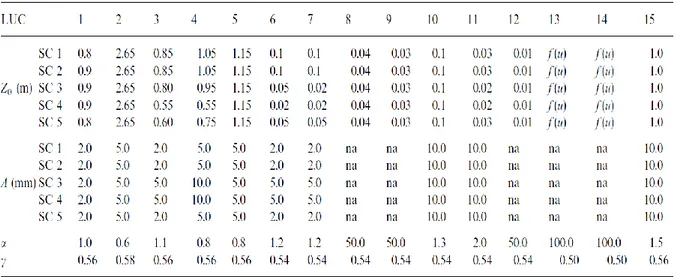
where is the collection efficiency from Brownian diffusion; the collection efficiency from impaction; the collection efficiency for interception; the correction factor representing the fraction of the particles that stick to the surface; and an empirical constant taken as 3 for all land use categories (LUC), reported in Tab. (2.1).
For Brownian diffusion, is a function of the parameter Sc evaluated by Eq. (2.22), and it is given as:
(2.27)
in which is function of the land use categories, as reported in Tab. (2.2). For impaction efficiency, EIM, the following relationship is used:
(2.28)
with chosen equal to 2 and varying with LUC, as reported in Tab. (2.2).
Stokes number, St, is the parameter governing impaction processes and it is calculated for vegetated surface as follows:
whereas for smooth or with bluff roughness elements surfaces:
(2.30)
where A is the characteristic radius collectors, (mm), and it is given for different land use and seasonal categories as reported in Tab. (2.2).
The following form is used for calculating collection efficiency by interception, :
(2.31)
Particles larger than 5 µm may rebound after hitting a surface. This process is included by modifying the total collection efficiency by the factor of R1, in Eq. (2.26). This parameter is calculated as:
(2.32)
Particles can grow in high humidity conditions. This effect is included here by replacing the dry particle radius with a wet one. The wet particle radius, , is calculated using the dry particle radius,
, and the relative humidity (Gerber, 1985) for sea-salt and sulphate aerosols:
(2.33)
where , , and are empirical constants using the values listed in Tab. (2.3).
Table 2.2 - Parameters for 12 land use categories (LUC) and five seasonal categories (SC)a reported in (Zhang et al., 2001)
Table 2.3 - Constants used in Eq. (2.33).
2.6 Chen et al. (2012) model
Based on their experimental results, Chen et al. (2012) developed a relationship between TSP (Total Suspended Particulate Matter) deposition velocity and meteorological parameters.
The experimental campaigns were conducted in locations near Guangzhou, China, during the dry season.
The deposition velocity is expressed as follow:
(2.34)
where u is the wind speed (m/s); is the relative humidity (%); and T is the temperature (°C).
Eq. (2.34) shows significant positive correlation between the dry deposition velocity and the wind speed, while the temperature and the relative humidity are negatively related.
Wind speed could be one of the strongest factors that determine the magnitude of particle dry deposition velocity.
Relative humidity has not a critical impact to the dry deposition velocity especially during the dry season. It may affect the dry deposition velocity only under certain meteorological conditions. Temperature is also a considerably important meteorological factor responsible for the change of the dry deposition velocity.
It’s important to note that local climate changes arising from either anthropogenic emissions or improper urban planning, tend to alter some meteorological parameters.
For instance, the urban heat island tends to raise the air temperature extensively while also reduce the relative humidity and wind speed in urban areas.
Therefore, it may consequently lead to changes in the TSP dry deposition velocity even in word widely.
2.7 Giardina et al. (2017) model
Giardina et al. (2017) proposed a new approach, based on the electrical analogy, to evaluate the total resistance rt to be used in Eq. (2.10), valid for urban rough surfaces
The scheme of deposition processes upon the canopy of urban surfaces has been modified to include the particle rebound or resuspension phenomena together with Brownian diffusion, impaction process, and turbulent transfer, as described in the following.
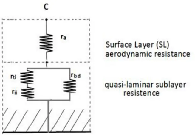
In the proposed approach the aerodynamic resistance, ra, is connected in series with the resistance across the quasi-laminar sublayer, rql, to take into account mechanisms of diffusion by Brownian motion and impaction phenomena (Fig. 2.2).
Fig. 2.2 - New schematization based on electrical analogy for parametrization of particles deposition velocity.
The resistance rql is evaluated by considering two resistances in parallel, that is: resistance rbd, which represents the Brownian diffusion; and the resistance ri, which allows to treat impaction processes. The resistance ri is evaluated by considering two resistances in series: rii that takes into account the inertial impact condition; rti that considers the effects resulting from turbulent impaction.
These last assumptions allow to take into consideration effects on particle concentration coming from both the inertial and turbulent impaction (i.e. reciprocal influence of the two impact processes on dry deposition efficiency).
Accordingly, the overall resistance, rt, in Eq. (2.10) is evaluated by the using the following equations: (2.35)
The aerodynamic resistance, is calculated by using Eq.s (2.6), (1.3), (1.4), whereas rql, using the electric analogy, is evaluated as:
(2.36)
(2.37)
For the resistance rbd, the Authors assumed the following expression:
= (2.38)
The transport of particles by Brownian diffusion represented as function of Sc2/3 in Eq. (2.38) is recommended in various works on the basis of theoretical and empirical results (Wesely and Hicks, 1977; Paw, 1983; Hicks et al., 1987; Pryor et al., 2009; Kumar and Kumari, 2012).
In order to evaluate the resistance for inertial impact process in Eq. (2.37), is used the following relationship valid for rough surfaces:
(2.39) The particle rebound in Eq. (2.39) is evaluated as follow:
(2.40) where is assumed b = 2.
The general assumptions made for the calculation of resistance rti are reported below.
Empirical relations of turbulent deposition are typically presented in terms of the dimensionless particle relaxation time τ+:
(2.41) where τ is the particle relaxation time defined, for a spherical particle, as follows:
τ (2.42)
Various models predict a functional dependence of resistance turbulent impact phenomena, rti, on + as follows:
(2.43)
The constants m and n in Eq. (2.43) have been evaluated by fitting some data reported in literature for urban surfaces. The results were 0.05 and 0.75, respectively. In this work the values of these parameters have been slightly modified on the bases of further sensibility analyses that have led to m=0.1 and n=0.5. These last values have been used for the validation activities reported in the following sections. In the light of the above considerations, Eq. (2.10) can be rewritten as follows:
(2.44)
where rdb, rii, and rti are evaluated by Eq.s (2.38), (2.39), (2.40), and (2.43). 2.8 Considerations about Brownian diffusion resistance
The model reported in (Giardina et al., 2017), has been tested by using two different Brownian diffusion resistances, rbd,.
The first has been proposed by Chamberlain et al. (1984), the second was derived from a sensibility analyses performed in this research activity.
2.8.1 Brownian diffusion resistance from Chamberlain et al. (1984)
In (Chamberlain et al., 1984) experiments were carried out to study diffusive transfer to bluff roughness elements that can be compared to urban et suburban conditions.
Radioactive gases and labelled particles were used in wind tunnels to measure the effects of Reynolds and Schmidt numbers on transport to surfaces with widely spaced roughness elements. Moreover, correlations were obtained for gases and for sub-micrometric sized particles.
It is highlighted that deposition of larger particles is dominated by the effects of bounce off, which depends on surface conditions.
The Authors defined the following non dimensional parameter for mass and momentum transport, :
(2.45)
and proposed the relationship to take into account the effects of Reynolds and Schmidt numbers: (2.46) where the roughness Reynolds number is defined as:
(2.47) Using Eq.s (1.2), (2.45), (2.46) and doing some math, the following expression for the resistance due to diffusion transport, rbd, can be found:
(2.48) 2.8.2 Brownian diffusion resistance from sensitive analysis
In literature various models allow to predict functional dependence of Brownian diffusion resistance, rbd, from Sc number and friction velocity, , however they cannot be used for different urban conditions.
In the field, research activities have been carried out to define a new formulation that is capable to perform predictions for different typologies of urban area and small particle diameters.
For this purpose, sensitive analyses were performed on parameters that associate Brownian diffusion resistance to Reynolds (Eq. 2.47) and Schmidt numbers.
These analyses were carried out by using experimental data of dry deposition velocity for different surfaces (Möller and Schumann, 1970; Sehemel and Sutter, 1974; Pryor et al., 2007; Pryor et al., 2009).
The following relationship was obtained:
3. VALIDATION WORK OF DRY DEPOSITION VELOCITY ON ITALIAN CITIES 3.1 Introduction
The validation works have been performed by using experimental campaigns carried out by researchers from ISAC-CNR unit of Lecce, covering for different surface roughness conditions, i.e. from the patchy Venice lagoon surface (on the island of Mazzorbo) to the near urban areas for Maglie (LE) and Bologna.
The data were made available in the context of the Research Agreement between ISAC-CNR and Department of Energy, Engineering of the information and Mathematical Models, University of Palermo.
These experiments, performed between 2004s and 2009s, have been grouped in classes of friction velocities, each other spaced of 0.1 m/s.
Displacement height, 𝑑, and the roughness height, 𝑧0,reported in Tab. (3.1) have been evaluated from micrometeorological measurements, following a method reported in (Toda and Sugita, 2013) which uses similarity relationship for sonic temperature and vertical wind component..
These data have been used for the application of the models reported in (Giardina et al., 2017), (Chen et al., 2012), (Noll et al., 2001), and (Zhang et al., 2001), that have been compared with the measured dry deposition velocities.
To deepen the work of these comparisons, dry deposition velocity experimental data reported in (Donateo and Contini, 2014), for the same sites of measure, have been added.
Table 3.1 - Summary of experimental sites and instruments used in aerosol sampling performed by ISAC-CNR. Measurement height (z), displacement height (d), and roughness length (z0) are
reported. Table adapted from (Donateo and Contini, 2014).
Site Instruments Height z (m) Displacement
height d (m) Roughness length z0 (m)
Venice lagoon pDR-1200Thermo-MIE 9.6 5.1 ± 0.5 land
0 water 0.11 ± 0.03 land 0.01 ± 0.03 water Bologna CPC Grimm 5.403 10 4.8± 0.5 0.35 ± 0.02 Lecce (2005) Lecce (2010) pDR-1200 Thermo-MIE CPC Grimm 5.43 10 6.1 ± 0.4 0.53 ± 0.02 Maglie pDR-1200 Thermo-MIE 10 6 ± 0.5 0.52 ± 0.02
3.2 Maglie urban site (South-Eastern Italy)
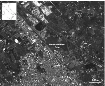
The measurement site, located in NE boundary of the town of Maglie (LE) in the Apulia region of Italy (40°07’38.39’’N, 18°17’59.50’’E), can be considered an urban background site influenced by an industrial area.
The town is extending mainly in the sector of wind direction between SE and SW and the country side is in the sector between NNO and E. In the town direction, the site is characterized by the presence of small buildings (1-2 floors) and roads with relatively high traffic volume (Fig. 3.1).
The monitoring campaigns of PM2.5 concentration measurements were performed during the period reported below:
13/01/2004 ÷ 30/01/2004; 26/11/2004 ÷ 26/12/2004; 24/11/2006 ÷ 16/12/2006; 28/11/2007 ÷ 07/12/2007.
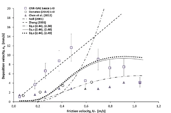
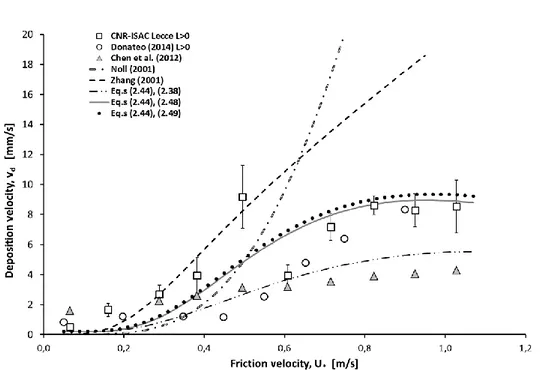
Fig.s (3.2) and (3.3) show the deposition velocity as function of friction speeds for unstable and stable conditions, respectively. These figures report comparisons among experimental data from ISAC-CNR, for the periods above described, experiments reported in (Donateo and Contini, 2014), and predictions obtained by applying the models reported in (Giardina et al., 2017), (Chen et al., 2012), (Noll et al., 2001), and (Zhang et al., 2001).
In all figures, error bars percentage of 25% has been reported for ISAC-CNR experimental data. The dry deposition velocities reported in (Donateo and Contini, 2014) are related to January 2004, December 2004, December 2006, December 2007 and September 2008.
It is possible to notice, even if the detection periods are the same (winter), in (Donateo and Contini, 2014) industrial area was taken to measurements, while the data of ISAC-CNR refer to the city zone . A screening was made on the data based on the wind direction. This justifies the difference between the experimental results reported in Fig. (3.2).
Zhang et al. (2001) model has been employed using the parameters reported in Tab.s (2.1) and (2.2), valid for urban area.
Figure 3.1 - Maglie, suburban area, the measurement point is reported. Adapted from Donateo and Contini (2014)
Figure 3.2 - Comparisons among dry deposition velocity experimental data for Maglie city with L<0, experiments reported in (Donateo and Contini, 2014) and the predictions obtained by using models reported in (Giardina et al., 2017), (Chen et al., 2012), (Noll et al., 2001), and (Zhang et al.,
2001).
The model of Chen et al. (2012) was applied by averaging the values of wind velocity, temperature and relative humidity measured during the experimental campaigns.
Giardina et al. (2017) model has been also tested by using in Eq. (2.44) and the relationships reported in Eq.s (2.48) and (2.49), related to different formulations for Brownian diffusion resistance, as described in sections 2.7 and 2.8.
Analyzing results, Zhang et al. (2001) model allows a good agreement with experimental data for friction velocities less than about 0.5 (m/s), however it does not follow the experimental trend for higher values. This last condition is especially true for the predictions obtained by using Noll et al. (2012) model.
Chen et al. (2012) model and Giardina et al. (2017) model, this last applied with Eq. (2.38), show a good agreement with the experimental data reported in (Donateo et al., 2014), but only for friction velocities below about 0.6 m/s. For friction velocities above this value, the predictions underestimate the experimental data.
Giardina et al. (2017) model shows very good agreements if it is applied with Brownian diffusion resistances reported in Eq.s (2.48) and (2.49). The two curves result very close both for unstable and stable conditions.
Figure 3.3 - Comparisons among dry deposition velocity experimental data for Maglie (city wind sector) with L>0, experiments reported in (Donateo and Contini, 2014) and the predictions obtained by using models reported in (Giardina et al., 2017), (Chen et al., 2012), (Noll et al., 2001),
and (Zhang et al., 2001). 3.3 Venice lagoon (Mazzorbo Island, North-Eastern Italy).
Measurements were performed at a background site placed on the island of Mazzorbo, in the Venice lagoon at 10 m above the ground (Fig. 3.4).
The measurement site (45°29’09.5’’N, 12°24’12.7’’E) was a field located at about 8 km NE of the Venice town.
This site was located very close (about 5 m) to the water lagoon at the W-SW side, while, in the other directions (north, east, and south), it was characterized by land for about 1-2 km with short vegetation, some small trees, and one or two-floor houses, although channels and water were also present in this area.
The monitoring campaigns of PM2.5 concentration and flux measurements were performed during the period reported below:
03/07/2004 ÷ 16/07/2004; 17/02/2005 ÷ 27/02/2005; 01/03/2005 ÷ 15/03/2005; 05/05/2006 ÷ 23/05/2006.
Fig.s (3.5) and (3.6), that report the deposition velocity as function of friction speed, refer to instability and stability atmospheric conditions, respectively.
These figures shown comparisons among experimental data from ISAC-CNR, experiments reported in (Donateo and Contini, 2014), and predictions obtained by using models reported in (Giardina et al., 2017), (Noll et al., 2001), and (Zhang et al., 2001).
Chen et al. (2012) model is not reported for experimental tests with unstable conditions due to lack of data in terms of temperatures and relative humidity.
Figure 3.4 - Venice lagoon, Mazzorbo island, the measurement point is reported. Adapted from Donateo and Contini (2014)
Figure 3.5 - Comparisons between the dry deposition velocity experimental data for Venice city with L<0 and the prediction obtained by using models reported in (Noll et al., 2011), (Zhang et al.,
2001), and (Giardina et al., 2017).
Giardina et al. (2017) model has been tested by using Eq.s (2.38), (2.48), and (2.49).
Very high differences can be highlighted between dry deposition velocities experimental data and the predictions of Zhang et al. (2001) model and Noll et al. (2001) one, both for unstable and stable conditions (Fig.s 3.5, 3.6).
The curves obtained by Giardina et al. (2017) model, applied with Eq.s (2.38), (2.48) and (2.49), show a very good agreement with experimental data reported in (Donateo and Contini, 2014), whereas overestimate the experiments from ISAC-CNR. The three curves result very close each other both for unstable and stable conditions.
For stable conditions, Chen et al. (2012) model underestimates the experimental tests of CNR-ISAC and overestimates those reported in (Donateo and Contini, 2014).
Figure 3.6 - Comparisons between the dry deposition velocity experimental data for Venice city with L>0 and the predictions obtained by using models reported in (Noll et al., 2011), (Zhang et al.,
2001), and (Giardina et al., 2017). 3.4 Bologna industrial district (Central Italy)
The measurement site, shown in Fig. (3.7), was near the incinerator plant for the city of Bologna, (44°31’17.59’’N, 11°25’53.48’’E), It is worth noted that in this case the number particle concentration has been measured, with particles diameter from 9 nm to 1 m (with a median value of 0.045 m). The data refer to experimental campaigns performed in summer and winter, as reported below:
06/06/2008 ÷ 22/07/2008; 21/01/2009 ÷ 10/03/2009.
Fig.s (3.8) and (3.9) report the deposition velocity experimental data as function of friction velocity for instability and stability atmospheric conditions, respectively.
In particular, these figures show the comparison among experiments of ISAC-CNR, experimental tests reported in (Donateo and Contini, 2014), and results obtained by using the models of Noll et al. (2001), Zhang et al. (2001), Chen et al. (2012) and Giardina et al. (2017).
The experiments reported in (Donateo and Contini, 2014) were carried out from June to July 2008, and January to March 2009 for the same particle diameters.
High differences can be highlighted between dry deposition velocities experimental data and the predictions of Zhang et al. (2001) model for unstable conditions (Fig. 3.8), however for stable conditions this is true for friction velocity above about 0.3 m/s (Fig. 3.9).
The predictions of Noll et al. (2001) model and Giardina et al. (2017) model, this last applied with Eq. (2.48), show very high underestimation for all experiments.
The curves obtained by Giardina et al. (2017) model, applied with Eq.s (2.38) and (2.49), show a good agreement with experimental data, however with a small underestimation from Giardina et al. (2017) model applied with Eq. (2.38).
Finally, comparisons with results obtained by applying Chen et al. (2012) model show a good agreement for both instability and stability atmospheric conditions, even if the predictions for unstable atmosphere conditions (Fig. 3.8) seem to change trend respect the dry deposition experimental data. In fact, dry deposition experimental data show an increasing trend with increasing friction speeds.
Figure 3.7 - Bologna, Frullo industrial district; the measurement point is reported. Adapted from Donateo and Contini (2014)
Figure 3.8 - Comparisons between the dry deposition velocity experimental data for Bologna city with L<0 and the results obtained by using models reported in (Noll et al., 2001), (Zhang et al., 2001),
(Chen et al., 2012), and (Giardina et al., 2017).
Figure 3.9 - Comparisons between the dry deposition velocity experimental data for Bologna city with L>0 and the results obtained by using models reported in (Noll et al., 2001), (Zhang et al., 2001),
(Chen et al., 2012), and (Giardina et al., 2017). 3.5 Lecce suburban site
Experimental campaigns were performed during spring/summer 2005 and 2010, from April until June relative. PM2.5 concentrations and fluxes were measured.
The site was the experimental field of the Lecce Unit of ISAC-CNR placed inside the University Campus (40°20‘10.8‘’N, 18°07‘21.0‘’E) and located at about 3.5 km SW from the town of Lecce. It is a
rectangular field with a major side of about 200 m characterized by short vegetation, with two contiguous sides surrounded by small trees (Fig. 3.10).
The urban background area is characterized for at least 1 km in all directions by the presence of patches of trees (8–10 m tall) and small two-storey buildings and some roads with no industrial releases nearby.
Due to the proximity of urban areas, the site can be categorized as an urban background area. Measurements were taken at 10 m above the ground.
Figure 3.10 - Lecce, University Campus, the measurement point is reported. Adapted from Donateo and Contini (2014)
Fig.s (3.11) and (3.12) show the deposition velocity as function of friction speeds for unstable and stable conditions reported in (Donateo and Contini, 2014), and predictions obtained by applying the models reported I (Noll et al., 2001), and (Zhang et al., 2001) and (Giardina et al., 2017).
Analyzing results, Zhang et al. (2001) model allows very high underestimations of dry deposition velocity experimental data for friction velocities higher than about 0.25 (m/s) and unstable conditions (Fig. 3.11). This condition is also present for stable conditions but for friction velocity higher than about 0.45 m/s (Fig. 3.12).
Noll et al. (2001) model allows a high underestimation of experimental data for friction velocities higher than about 0.5 (m/s), for both unstable and instable conditions.
Giardina et al. (2017) model, applied with Eq.s (2.38), (2.48), and (2.19) show a good agreement with all experimental data. The three curves result very close each other, both for unstable and stable conditions.
Figure 3.11 - Comparisons between the dry deposition velocity experimental data for Lecce city with L<0 and models by (Noll et al., 2001), Zhang (2001), and Giardina et al. (2017).
Figure 3.12 - Comparisons between the dry deposition velocity experimental data for Lecce city with L>0 and models by (Noll et al., 2001), Zhang (2001), and Giardina et al. (2017)
4. VALIDATION WORK OF DRY DEPOSITION VELOCITY ON UNITED STATES URBAN AREAS 4.1 Introduction
As previously discussed, dry deposition phenomena modelling on urban canopies is limited and, although empirical or semi-empirical models have been developed to address this complex issue, there is no universal acceptance criteria. Therefore, it can be said that the models proposed in literature are not capable of representing particle dry deposition for several categories of pollutants and different urban surface geometries.
In order to overcome these problems, validations works by using experimental campaigns on different urban canopies, but also in other parts of the world compared to Italy, have been performed.
In this section the results obtained on typical United States urban areas are shown and discussed. It is to be noted that the roughness length z0 for the examined urban areas were evaluated by using Devenport classification reported in Tabs (1.2) and (1.3) if this data were not reported by the Authors in their paper.
4.2 Experimental data of Noll et al. (2001)
Four sampling campaigns conducted at Chicago are described in (Noll et al., 2001). The data were collected on the roof of a four-story building (12 m height) located in a mixed institutional, commercial, and residential area on the south of Chicago.
The building is located on the IIT (Illinois Institute of Technology) campus, which is located 5.6 km south of Chicago’s center and 1.6 km west of Lake Michigan. The IIT campus consists of predominately low rise buildings, landscaped areas, and asphalt parking lots.
The atmospheric particle mass size distribution and dry deposition flux were measured simultaneously with a wide range aerosol classifier (WRAC) and a smooth greased surface.
Data summary for samples collected from Chicago-IIT site are reported in Tab. (4.1).
The Authors have used the results of experimental data to develop the relationship reported in Eq. (2.23) for dry deposition velocity calculations.
Fig. (4.1) reports the experimental dry deposition velocity as function of particle diameters and Fig. (4.2) the dimensionless dry deposition velocity (vd+=vd/u*) as function of dimensionless particle relaxation time τ+. Both figures are reported in log-log graphs.
Comparisons with the results obtained by using models reported in (Noll et al., 2001) and (Giardina et al., 2017) are also shown.
As expected, Noll et al. (2001) predictions show a good agreement with the experimental data reported in Fig. (4.1), while the model of Giardina et al. (2017), applied with Eq.s (2.48) and (1.49), underestimate the experimental data if the particle diameter is less than 10 m. If the rebound process is not considered (i.e. it is imposed R = 1 in Eq. 2.40), the predictions are improved even for particle diameters larger than 10 m.
It is worth to be noted that the model of Giardina et al. (2017), applied with Eq. (2.49), predicts, for diameters less than 1 μm, higher deposition rates than those obtained by applying the other two models (Fig. 4.1).
The comparisons of results reported in Fig. (4.2) allow to state that the model of Giardina et al. (2017), applied with Eq. (2.49), is in accordance with the trend of the dry deposition velocities for lower values of + equal to 1, to which corresponds a particle diameter of about 2 μm.
Table 4.1 - Data summary for samples collected from Chicago-IIT site.
Figure 4.1 - Comparisons between the dry deposition velocity, reported in (Noll et al., 2001) as function of particle diameters, and the results obtained by using models of Noll et al. (2001) and Giardina et al. (2017).
Figure 4.2 - Comparisons between the dimensionless dry deposition velocity, reported as function of dimensionless particle relaxation time τ+, with the results obtained by using models reported in (Noll et al., 2001) and (Giardina et al., 2017).
4.3 Experimental data of (McNeary and Baskaran, 2003)
The depositional fluxes in the bulk and dry fallout as well as the concentrations of 7Be and 210Pb in aerosols were measured for a period of 17 months at Detroit, Michigan.
The bulk depositional fluxes of 7Be and 210Pb varied between 3.11 and 63.0 dpm/cm2yr and 0.35 and 10.3 dpm/cm2yr, respectively, and this variability in the depositional fluxes is attributed to the frequency and amount of precipitation and seasonal variations in the depositional fluxes.
The dry depositional fluxes of 7Be and 210Pb contributed 2.1–19.8% and 3.6– 48.6% of the bulk depositional fluxes.
The sampling site is one of the air monitoring network stations operated by the Wayne County Air Quality Management Division and jointly operated by the Wayne County and the Michigan Department of Environmental Quality (MDEQ), under cooperative agreement with the U.S. Environmental Protection Agency (EPA).
A bulk rain collector (200-L polyethylene drum with surface area of 2800 cm2) was deployed in September 1999 at a site in the southwest area of Detroit, Michigan (42°250’N; 83°10’W; 175 m above mean sea level) at about 1 m above the ground to prevent the resuspension of dust particles getting into the collector. The lid of the bulk collector was deployed as the dry collector in October 1999 on the roof of a building at the same site at about 4 m above ground.
The bulk rain samples were collected after each major precipitation event or once in about a month and after about 10 days of dry weather for the dry collector.
Fig.s (4.3) and (4.4) report comparisons between dry deposition experimental data, during the period reported in Tab. (4.2), and predictions of the model proposed in (Giardina et al., 2017) by using Brownian diffusion resistance Eq.s (2.48) and (2.49), for two different particle diameter, dp = 0.1 and 1 m, respectively.
The wind speeds, used for model applications, are related to mesurements by meteorological station located near Detroit airport (Windsor). This station is the closer site to the measurement point. The calculation of the average of wind speed data for the period of measurements have been reported by Authors.
As we can see In Fig. (4.49), if the particle diameter increases, the calculated dry deposition rate increases, however, for some period, a underestimation of dry deposition velocity remains.
It should be highlighted that this comparison must be performed taking into account that the experimental measurements were carried out during rainy days, so these weather conditions can only increase deposition processes compared to dry deposition phenomena.
Figure 4.3 - Comparisons between dry deposition experimental data, during the period reported in Tab. (4.2), and the predictions of the model proposed in (Giardina et al., 2017)
by using Brownian diffusion resistances Eq.s (2.48) and (2.49) with particle diameter dp = 0.1 m
Figure 4.4 - Comparison between dry deposition experimental data, during the period reported in Tab. (4.2), and the predictions of the model proposed in (Giardina et al., 2017)
by using Brownian diffusion resistances Eq.s (2.48) and (2.49) and particle diameter dp = 1 m Table 4.2 Total Deposition Velocity of Aerosols Using 7Be and 210Pb
4.4 Experimental data of Aluko and Noll (2006)
Processes of both deposition and suspension velocities for large airborne particles (greater than 10 μm diameter) were investigated in (Aluko and Noll, 2006). These experiments were conducted in an urban area (Chicago, Illinois), removed from close by point sources of particles (site is located in the middle of IIT) campus and four blocks from the freeway) and at an elevation of 12 m, so that large particles generated in the vicinity of the sampling site are well entrained in the atmosphere before they were collected. The sampling site is 5.6 km south of the urban center and 1.6 km west of Lake Michigan.
The coarse particle airborne concentration was measured with a Noll Rotary Impactor that collects large particles by moving four rectangular collector stages of different dimensions through the aerosol at high speeds, relative to expected wind speeds.
The collector widths and velocity of rotation were varied to achieve different collection efficiencies. The airborne concentration of coarse particles was measured with a Rotary Impactor simultaneously with the measurement of particle dry deposition flux to a smooth surrogate surface with a sharp leading edge, mounted on a wind vane.
The mass median aerodynamic diameter (MMDa) and standard geometric deviation were calculated for the coarse particle mass concentration distribution, based on the measurement of the mass on the four Impactor stages. Simultaneously to airborne concentration particles measurement was used a deposition plate to measure the particle dry deposition flux. It was made from polyvinyl chloride (PVC), 16 cm long, 7.6 cm wide, and 0.55 cm thick, with a sharp leading edge (less than a 10 degree angle) that was pointed into the wind by a wind vane. One film was placed on the upper surface of the plate; the second film was directly below the upper film on the lower side of the plate.
Particle mass size distributions and downward and upward flux plate samples were collected simultaneously in two time periods: 8-hour daytime samples (approximately 08:00 to 16:00) and 16-hour night time samples (approximately 16:00 to 08:00). The collection of day and night samples allowed a wide range of atmospheric conditions to be evaluated because wind speeds during the day are generally higher than at night.
Continental flow (westerly winds) provided different sources and transport times for the collected particles.
Table 4.3 reports ambient particle concentration and dry deposition data by sampling categories. In Fig.s (4.5) and (4.6) the experimental data in terms of deposition flux during diurnal or nocturnal periods are shown. These figures report comparisons with Giardina et al. (2017) model, by using Eq.s (2.44) and (2.49). The results show that the model allows to predict the measured fluxes with errors that slightly exceed the 20%.
Figure 4.5 - Comparison between experimental data of deposition for Continental flow, during the day, and predictions of the model proposed in (Giardina et al., 2017).
Figure 4.6 - Comparison between experimental data of deposition for Continental flow, during the day, and predictions of the model proposed in (Giardina et al., 2017).
It is worth to be noted that Eq.s (2.48) or (2.49) used in Giardina et al. (2017) model have provided very close results. This is justified by observing that the experimental measures are related to very high particle diameters, so the gravitational settling is dominant, whereas the contributions of Brownian diffusion resistance is insignificant.