2020-12-03T12:24:12Z
Acceptance in OA@INAF
The ALMA Spectroscopic Survey in the Hubble Ultra Deep Field: Evolution of the
Molecular Gas in CO-selected Galaxies
Title
Aravena, Manuel; DECARLI, ROBERTO; Gónzalez-López, Jorge; Boogaard,
Leindert; Walter, Fabian; et al.
Authors
10.3847/1538-4357/ab30df
DOI
http://hdl.handle.net/20.500.12386/28648
Handle
THE ASTROPHYSICAL JOURNAL
Journal
882
The ALMA Spectroscopic Survey in the
Hubble Ultra Deep Field: Evolution of the
Molecular Gas in CO-selected Galaxies
Manuel Aravena1 , Roberto Decarli2 , Jorge Gónzalez-López1 , Leindert Boogaard3 , Fabian Walter4,5 , Chris Carilli5 , Gergö Popping4 , Axel Weiss6 , Roberto J. Assef7 , Roland Bacon8, Franz Erik Bauer9,10,11 , Frank Bertoldi12 , Richard Bouwens3 , Thierry Contini13 , Paulo C. Cortes14,15 , Pierre Cox16, Elisabete da Cunha17, Emanuele Daddi18 ,
Tanio Díaz-Santos7, David Elbaz18, Jacqueline Hodge3 , Hanae Inami19, Rob Ivison20,21 , Olivier Le Fèvre22, Benjamin Magnelli12 , Pascal Oesch23,24 , Dominik Riechers4,25 , Ian Smail26 , Rachel S. Somerville27,28,
A. M. Swinbank26 , Bade Uzgil4,5 , Paul van der Werf3, Jeff Wagg29, and Lutz Wisotzki30 1
Núcleo de Astronomía, Facultad de Ingeniería y Ciencias, Universidad Diego Portales, Av. Ejército 441, Santiago, Chile;[email protected] 2
INAF–Osservatorio di Astrofisica e Scienza dello Spazio, via Gobetti 93/3, I-40129, Bologna, Italy
3
Leiden Observatory, Leiden University, P.O. Box 9513, NL2300 RA Leiden, The Netherland
4
Max Planck Institute für Astronomie, Königstuhl 17, D-69117 Heidelberg, Germany
5
National Radio Astronomy Observatory, Pete V. Domenici Array Science Center, P.O. Box O, Socorro, NM 87801, USA
6
Max-Planck-Institut für Radioastronomie, Auf dem Hügel 69, D-53121 Bonn, Germany
7
Núcleo de Astronomía, Facultad de Ingeniería, Universidad Diego Portales, Av. Ejército 441, Santiago, Chile
8Univ. Lyon 1, ENS de Lyon, CNRS, Centre de Recherche Astrophysique de Lyon(CRAL) UMR5574, F-69230 Saint-Genis-Laval, France 9
Instituto de Astrofísica, Facultad de Física, Pontificia Universidad Católica de Chile Av. Vicuña Mackenna 4860, 782-0436 Macul, Santiago, Chile
10
Millennium Institute of Astrophysics(MAS), Nuncio Monseñor Sótero Sanz 100, Providencia, Santiago, Chile
11
Space Science Institute, 4750 Walnut Street, Suite 205, Boulder, CO 80301, USA
12
Argelander-Institut für Astronomie, Universität Bonn, Auf dem Hügel 71, D-53121 Bonn, Germany
13
Institut de Recherche en Astrophysique et Planétologie(IRAP), Université de Toulouse, CNRS, UPS, F-31400 Toulouse, France
14
Joint ALMA Observatory—ESO, Av. Alonso de Córdova, 3104, Santiago, Chile
15
National Radio Astronomy Observatory, 520 Edgemont Road, Charlottesville, VA, 22903, USA
16
Institut d’Astrophysique de Paris, 98 bis boulevard Arago, F-75014 Paris, France
17
Research School of Astronomy and Astrophysics, Australian National University, Canberra, ACT 2611, Australia
18
Laboratoire AIM, CEA/DSM-CNRS-Universite Paris Diderot, Irfu/Service d’Astrophysique, CEA Saclay, Orme des Merisiers, F-91191 Gif-sur-Yvette cedex, France
19
Hiroshima Astrophysical Science Center, Hiroshima University, 1-3-1 Kagamiyama, Higashi-Hiroshima, Hiroshima 739-8526, Japan
20
European Southern Observatory, Karl-Schwarzschild-Strasse 2, D-85748, Garching, Germany
21
Institute for Astronomy, University of Edinburgh, Royal Observatory, Blackford Hill, Edinburgh EH9 3HJ, UK
22
Aix Marseille Université, CNRS, LAM(Laboratoire d’Astrophysique de Marseille), UMR 7326, F-13388 Marseille, France
23
Department of Astronomy, University of Geneva, Ch. des Maillettes 51, 1290 Versoix, Switzerland
24
International Associate, Cosmic Dawn Center(DAWN) at the Niels Bohr Institute, University of Copenhagen and DTU-Space, Technical University of Denmark, Denmark
25
Cornell University, 220 Space Sciences Building, Ithaca, NY 14853, USA
26Centre for Extragalactic Astronomy, Department of Physics, Durham University, South Road, Durham, DH1 3LE, UK 27
Department of Physics and Astronomy, Rutgers, The State University of New Jersey, 136 Frelinghuysen Road, Piscataway, NJ 08854, USA
28
Center for Computational Astrophysics, Flatiron Institute, 162 5th Avenue, New York, NY 10010, USA
29
SKA Organization, Lower Withington Macclesfield, Cheshire SK11 9DL, UK
30
Leibniz-Institut für Astrophysik Potsdam(AIP), An der Sternwarte 16, D-14482 Potsdam, Germany Received 2019 March 19; revised 2019 July 5; accepted 2019 July 10; published 2019 September 11
Abstract
We analyze the interstellar medium properties of a sample of 16 bright CO line emitting galaxies identified in the ALMA Spectroscopic Survey in the Hubble Ultra Deep Field(ASPECS) Large Program. This CO−selected galaxy sample is complemented by two additional CO line emitters in the UDF that are identified based on their Multi-Unit Spectroscopic Explorer(MUSE) optical spectroscopic redshifts. The ASPECS CO−selected galaxies cover a larger range of star formation rates(SFRs) and stellar masses compared to literature CO emitting galaxies at z>1 for which scaling relations have been established previously. Most of ASPECS CO-selected galaxies follow these established relations in terms of gas depletion timescales and gas fractions as a function of redshift, as well as the SFR–stellar mass relation (“galaxy main sequence”). However, we find that ∼30% of the galaxies (5 out of 16) are offset from the galaxy main sequence at their respective redshift, with ∼12% (2 out of 16) falling below this relationship. Some CO-rich galaxies exhibit low SFRs, and yet show substantial molecular gas reservoirs, yielding long gas depletion timescales. Capitalizing on the well-defined cosmic volume probed by our observations, we measure the contribution of galaxies above, below, and on the galaxy main sequence to the total cosmic molecular gas density at different lookback times. We conclude that main-sequence galaxies are the largest contributors to the molecular gas density at any redshift probed by our observations (z∼1−3). The respective contribution by starburst galaxies above the main sequence decreases from z∼2.5 to z∼1, whereas we find tentative evidence for an increased contribution to the cosmic molecular gas density from the passive galaxies below the main sequence.
Key words: galaxies: evolution– galaxies: ISM – galaxies: star formation – galaxies: statistics © 2019. The American Astronomical Society. All rights reserved.
1. Introduction
One of the major goals of galaxy evolution studies has been to understand how galaxies transform their gas reservoirs into stars as a function of cosmic time, and how they eventually halt their star formation activity.
An important development has been the discovery that most of the star-forming galaxies show a tight correlation between their stellar masses and star formation rates (SFRs; e.g., Brinchmann et al. 2004; Daddi et al. 2007; Elbaz et al.
2007,2011; Noeske et al.2007; Peng et al.2010; Rodighiero et al.2010; Whitaker et al.2012,2014; Schreiber et al.2015).
Galaxies in this sequence, usually called “main-sequence” (MS) galaxies, would form stars in a steady state for ∼1–2 billion years and dominate the cosmic star formation activity. Galaxies above this sequence, forming stars at higher rates for a given stellar mass, are called “starbursts”; and galaxies below this sequence, are called“passive” or “quiescent” galaxies. The large gas reservoirs necessary to sustain the star-forming activity along the MS would be provided through a continuous supply from the intergalactic medium and minor mergers (Kereš et al. 2005; Dekel et al.2009). As a consequence, the
fundamental galaxy parameters (SFRs, stellar masses, gas fractions, and gas depletion timescales) are found to be closely related at different redshifts. Galaxies above the MS have boosted their SFRs typically through a major merger event (e.g., Kartaltepe et al. 2012).
A critical parameter in the interstellar medium (ISM) characterization has been the specific SFR (sSFR), defined as the ratio between the SFR and stellar mass(SFR/Mstars), which
for a linear scaling between these parameters denotes how far a galaxy is from the MS population at a given redshift and stellar mass. As a result of observations of gas and dust in star-forming galaxies at high redshift in the last decades (for a detailed summary, see Tacconi et al. 2018; Freundlich et al.
2019), current studies indicate that there is an increase of the
gas depletion timescales and a decrease in the molecular gas fractions with decreasing redshift(z∼3 to 1), and that the gas depletion timescales decrease with increasing sSFR (Bigiel et al. 2008; Daddi et al. 2010a, 2010b; Genzel et al.
2010,2015; Tacconi et al.2010,2013,2018; Saintonge et al.
2011b, 2013, 2016; Leroy et al. 2013; Santini et al. 2014; Sargent et al. 2014; Papovich et al. 2016; Schinnerer et al.
2016; Scoville et al. 2016, 2017; Freundlich et al. 2019; Wiklind et al.2019). Finally, after galaxies would have formed
most of their stellar mass on and above the MS, they would slow down or even halt star formation when they exhausted most of their gas reservoirs (e.g., Peng et al. 2010), bringing
them below the MS line.
Observations of the cold molecular gas in high-redshift galaxies have typically relied on transitions of carbon monoxide,12CO(hereafter CO), to infer the existence of large gas reservoirs, as CO is the second most abundant molecule in the ISM of star-forming galaxies after H2 and given the
difficulty in directly detecting H2 (Solomon & Vanden
Bout2005; Omont 2007; Carilli & Walter2013).
While progress has been substantial, there are still potential biases that have so far been little explored. For example, most of the high-redshift galaxies for which observations of molecular gas and dust are available have been preselected from optical and near-IR extragalactic surveys, based on their stellar masses and SFRs estimated from spectral energy distribution (SED) fitting or UV/24 μm photometry. Also
due to the finite instrumental bandwidth of millimeter interferometers, CO line studies rely on optical/near-IR redshift measurements. In most cases this means that galaxies need to have relatively bright emission or absorption lines, or display strong features in the continuum. Similarly, galaxy selection based on detections in Spitzer and Herschel far-IR maps, or in ground-based submillimeter observations, will target the most strongly star-forming galaxies, and are in many cases affected by source blending due to the poor angular resolution of these space missions. In turn, this means that such source preselection will select massive galaxies on or above the massive end of the MS.
A complementary approach to the targeted observations has been the so-called “molecular line scan” strategy (Carilli & Blain 2002; Walter et al. 2014). Here, millimeter/centimeter
line observations of an extragalactic “blank-field” are per-formed using a sensitive interferometer, exploring a significant frequency range(e.g., the full 3 mm and/or 1 mm band) over a sizable area of the sky. This essentially provides a large data cube to search for the redshifted emission from CO emission lines and/or cold dust continuum. Under this approach, galaxies are selected purely based on their molecular gas content. Pioneering observations of the Hubble Deep Field North (HDF-N) with the Plateau de Bureau Interferometer, covering the full 3 mm band, led to thefirst estimates of the CO luminosity functions (LF) at high redshift and the first constraints on the cosmic density of molecular gas (Decarli et al. 2014; Walter et al. 2014). More recently, observations
with the Karl Jansky Very Large Array at centimeter wavelengths in the COSMOS field and the HDF-N have allowed to cover larger areas, enabling the characterization of larger samples of gas rich galaxies, and providing tighter constraints on the CO LF and the evolution of the cosmic density of molecular gas (Pavesi et al. 2018; Riechers et al.
2019).
The ALMA Spectroscopic Survey (ASPECS) is the first contiguous molecular survey of distant galaxies performed with ALMA. The ASPECS pilot program targeted a region of 1 arcmin2of the Hubble Ultra Deep Field(HUDF), scanning the full 3 mm and 1 mm bands. This enabled independent line searches in each band (Walter et al. 2016), allowing the
investigation of a variety of topics including the characteriza-tion of CO-selected galaxies(Decarli et al.2016a), constraints
on the CO LF and cosmic density of molecular gas (Decarli et al. 2016b), derivation of 1 mm continuum number counts
and study of the properties of the faintest dusty galaxies (Aravena et al.2016b; Bouwens et al.2016), searches for [CII]
line emission at z>6 (Aravena et al.2016c), and derivation of
constraints for CO intensity mapping experiments(Carilli et al.
2016).
The ASPECS program has since been expanded, represent-ing thefirst extragalactic ALMA large program (LP). ASPECS LP builds upon the observational strategy and the results presented by the ASPECS pilot observations, but extending the covered area of the HUDF from ∼1 arcmin2 to 5 arcmin2, comprising the full area encompassed by the Hubble eXtremely Deep Field(XDF). We here report results based on the 3 mm data obtained as part of the ASPECS LP.
The ASPECS LP survey strategy and derivation of the CO LF and evolution of the cosmic molecular gas density are presented by Decarli et al. (2019). The line and continuum
number counts are presented in González-López et al. (2019).
The optical source and redshift identification and global galaxy properties, based on the ultra deep optical/near-IR coverage of the UDF are presented in Boogaard et al.(2019). A theoretical
prediction of the cosmic evolution of the CO LF and comparison to the ASPECS measurements are presented in Popping et al.(2019).
In this paper, we analyze the ISM properties of the 16 statistically reliable CO line identifications plus 2 lower significance CO lines identified through optical redshifts, and compare them with the properties of previous targeted CO observations at high redshift. In Section 2, we briefly summarize the ASPECS LP observations and the ancillary data used in this work. In Section 3, we present the CO line properties. In Section4, we compare the ISM properties of our ASPECS CO galaxies with standard scaling relations derived from targeted observations of star-forming galaxies. In Section5, we summarize the main conclusions from this work. Hereafter, we assume a standard ΛCDM cosmology with H0=70 km s−1Mpc−1,ΩΛ=0.7, and ΩM=0.3.
2. Observations
The ASPECS LP uses the same observational strategy followed by the ASPECS pilot survey(Walter et al.2016), but
expanding the covered area to ∼5 arcmin2. The ASPECS approach is to perform frequency scans over the ALMA bands 3 and 6 (corresponding to the atmospheric bands at 85–115 GHz and 212–272 GHz, respectively) and mapping the selected area through mosaics. The overall strategy is to search in this data cube for molecular gas rich galaxies through their redshifted12CO emission lines entering the ALMA bands. The ASPECS LP band 3 survey setup and data reduction steps are discussed in detail by Decarli et al.(2019). Details about the
line search procedures are presented in González-López et al. (2019). For completeness, we repeat the most relevant
information for the analysis presented here. 2.1. ALMA band 3
ALMA band 3 observations were obtained during Cycle 4 as part of the LP project 2016.1.00324.L. The observations were performed using a 17-point mosaic centered at (R.A., decl.)=(03:32:38.0, −27:47:00) in the HUDF. We used the spectral scan mode, covering the ALMA band 3, from 84.0 to 115.0 GHz in 5 frequency setups. This strategy yielded an areal coverage of 4.6 arcmin2 at 99.5 GHz at the half power beamwidth of the mosaic. Observations were performed in a compact array configuration, C40-3, yielding a synthesized beam of 1 75″×1 49 at 99.5 GHz.
The data were calibrated and imaged using the CASA
software, using an independent procedure, which follows the ALMA pipeline closely. The visibilities were inverted using the TCLEAN task. Since no very bright sources are found in the data cube, we used the “dirty” cubes. The data were rebinned to a channel resolution of 7.813 MHz, corresponding to 23.5 km s−1at 99.5 GHz. Thefinal cube reaches a sensitivity of∼0.2 mJy beam−1per 23.5 km s−1channel, yielding 5σ CO line sensitivities of ∼(1.4, 2.1, 2.3)×109K km s−1pc2 for CO(2−1), CO(3−2) and CO(4−3), respectively (Decarli et al.
2019). Our ALMA band 3 scan provides coverage for the
redshifted line emission from CO(1−0), CO(2−1), CO(3−2) and CO(4−3) in the redshift ranges 0.003–0.369, 1.006–1.738,
2.008–3.107, and 3.011–4.475, respectively (Walter et al.
2016; Decarli et al.2019).
2.2. CO Sample
To inspect the data cubes we used the LineSeeker line search routine (González-López et al. 2017). This algorithm
convolves the data along the frequency axis with an expected input line width, reporting pixels with signal-to-noise (S/N) values above a certain threshold. Kernel widths ranging from 50 to 500 km s−1 were adopted. The probability of each line candidate of not being due to noise peaks, or Fidelity, F, was assessed by using the number of negative line sources in the data cube, with F=1−NNeg/NPos. Here, NNeg and NPos
correspond to the number of negative and positive emission line candidates with a given S/N value in a particular kernel convolution (González-López et al. 2019). We select the
sources for which the fidelity is above 0.9. This yields 16 selected line candidates. All of them, except two sources have fidelity values of 1.0. We find that 3 mm.15 and 3 mm.16 have fidelity values of 0.99 and 0.92, respectively. All these sources are very unlikely to be false positives, based on the statistics presented by González-López et al. (2019). Two other
independent line searches were performed using similar algorithms with thefindclumps (Decarli et al.2016a; Walter et al. 2016) and MF3D (Pavesi et al. 2018) codes. All the
algorithms coincide in the statistical reliability of these sources. As we mention below, all the selected sources have reliable and matching optical/near-infrared counterparts. The sample of 16 line candidates thus constitutes our primary sample, all of which have S/N>6.4.
Two additional sources were selected based on the availability of an optical spectroscopic redshift and a matching positive line feature in the ALMA cube at the corresponding frequency. By construction, these sources are selected at lower significance than the CO-selected sources. For more details please refer to Boogaard et al.(2019). This makes up a sample
of 18 galaxies detected in CO emission by the ASPECS program in band-3.
2.3. Ancillary Data and SEDs
Our ALMA observations cover roughly the same region as the Hubble XDF. Available data include Hubble Space Telescope (HST) Advanced Camera for Surveys and Wide Field Camera 3 IR data from the HUDF09, HUDF12, and Cosmic Assembly Near-infrared Deep Extragalactic Legacy Survey(CANDELS) programs, as well as public photometric and spectroscopic catalogs (Coe et al. 2006; Xu et al. 2007; Rhoads et al.2009; McLure et al.2013; Schenker et al. 2013; Bouwens et al. 2014; Skelton et al. 2014; Momcheva et al.
2015; Morris et al.2015; Inami et al.2017). In this study, we
make use of this optical and infrared coverage of the XDF, including the photometric and spectroscopic redshift informa-tion available from Skelton et al.(2014). The area covered by
the ASPECS LP footprint was observed by the Multi-Unit Spectroscopic Explorer (MUSE) Hubble Ultra Deep Survey (Bacon et al.2017), representing the main optical spectroscopic
sample in this area(Inami et al.2017). The MUSE at the ESO
Very Large Telescope provides integral field spectroscopy in the wavelength range 4750–9350 Å of a 3′×3′ region in the HUDF, and a deeper 1′×1′ region, which mostly overlaps with the ASPECS field. The MUSE spectroscopic survey
provides spectroscopic redshifts for optically faint galaxies at the ∼30 mag level, and is thus very complimentary to our ASPECS survey. In addition to the HST coverage, a wealth of optical and infrared coverage from ground-based telescopes is available in this field, including the Spitzer Infrared Array Camera(IRAC) and Multiband Imaging Photometer (MIPS), as well as by the Herschel PACS and SPIRE photometry (Elbaz et al. 2011). From this, we created a master photometric and
spectroscopic catalog of the XDF region as detailed in Decarli et al. (2019), which includes >30 bands for ∼7000 galaxies,
475 of which have spectroscopic redshifts.
We fit the SED of the continuum-detected galaxies using the high-redshift extension of MAGPHYS (da Cunha et al.
2008,2015), as described in detail in Boogaard et al. (2019).
We use the available broad- and medium-band filters in the optical and infrared regimes, from the U band to Spitzer IRAC 8 μm, including also the Spitzer MIPS 24 μm and Herschel PACS 100μm and 160 μm. We also include the ALMA 1.2-mm and 3.0-1.2-mm dataflux densities from Dunlop et al. (2017)
and González-López et al. (2019); however, we note that the
optical/infrared data have a much stronger weight given the tighter constraints in this part of the spectra. We do not include Herschel SPIRE photometry in the fits because its angular resolution is very poor, being almost the size of our targetfield for some of the IR bands. For each individual galaxy, we perform SED fits to the photometry fixed at the CO redshift.
MAGPHYS employs a physically motivated prescription to balance the energy output at different wavelengths.MAGPHYS
delivers estimates for the stellar mass, SFR, dust mass, and IR luminosity. Estimates on the IR luminosity and/or dust mass come from constraints on the dust-reprocessed UV light, which is well sampled by the UV-to-infrared photometry. The derived parameters are listed in Table2.
3. Results 3.1. CO Measurements
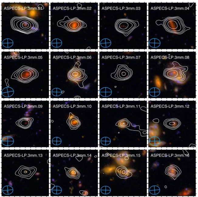
By construction, the ASPECS CO-based sources presented here are selected through their high significance CO line detection. The moment-0 images for each galaxy are created by collapsing the data cube along the frequency axis, considering all the channels within the 99.99% percentile range of the line profile. Figure 1 shows a combined CO image of all the moment-0 maps of these sources, highlighting the location of each of these sources in the field. This map is obtained by coadding all the individual moment-0 line maps, after masking all the pixels with S/N below 2.5σ. Figure 2 shows the CO spectral profiles, obtained at the peak position of each of the sources (see also AppendixB).
Following González-López et al. (2019), the total CO
intensities were derived from the ASPECS band-3 data cube by creating moment-0 images, collapsing the cube in velocity around the detected CO lines, and spatially integrating the emission from pixels within a region containing the CO emission(see González-López et al.2019, for more details).
All of our CO sources are clearly identified with optical counterparts, as described in detail by Boogaard et al. (2019).
While for most of these sources a photometric redshift is enough to provide an identification of the actual CO line transition and redshift, a large fraction of them is matched with a MUSE spectroscopic redshift. In three cases (3 mm.8, 3 mm.12, and 3 mm.15), the CO line emission can be either
associated with multiple optical sources, due to the higher angular resolution of the optical HST images, or the candidate CO redshift does not coincide with any of the cataloged photometric or spectroscopic redshifts. In these cases, inspec-tion of the MUSE data cube is critical(Boogaard et al.2019).
For the source 3 mm.13, identified with a CO(4−3) source at z∼3.601 we search for a nearby [CI] 1–0 emission line;
however, no emission is found at the explored frequency range (see AppendixA). Table 1lists the CO fluxes, positions, and derived CO redshifts.
We compute the CO luminosities,LCO¢ in units of K km s−1pc2, following Solomon et al.(1997):
( ) ( )
n
¢ = ´ - +
-LCO 3.25 107 r2 1 z 3D FL2 CO, 1 whereνris the rest frequency of the observed CO line, in GHz, DL
is the luminosity distance at redshift z, in Mpc, and FCO is the
integrated CO line flux in Jy km s−1. Following Decarli et al. (2016a), we convert the CO luminosities observed at transition
CO( -J J 1) to the ground transition CO(J=1−0) assum-ing a line brightness temperature ratio,rJ1= ¢LCOJ -J 1 LCO 1 0¢ – . From previous observations of massive MS galaxies(Daddi et al.
2015), we adopt r21=0.76±0.09, r31=0.42±0.07, and
r41=0.31±0.06. The uncertainties in LCO¢ account for the uncertainties in theflux measurements and for the uncertainties due to dispersion in the average rJ1 values measured by Daddi
et al. (2015). Since the Daddi et al. (2015) observations do not
measure the CO(4−3) lines, but rather CO(3−2) and CO(5−4), we extrapolate between those two lines(i.e., we follow the same approach as Decarli et al.2016b). We note that so far the Daddi
Figure 1.Rendered CO image toward the HUDF, obtained by coadding the individual average CO line maps around the 16 bright CO-selected galaxies and the 2 lower significance MUSE-based CO sources (labeled MP). Regions with significances below 2.5σ in each of the average maps are masked out prior to combination. The location of these individual detections is highlighted by solid circles and their IDs. The tendency of sources to lie in the top two-thirds of the map is likely a combination of clustering and chance, given the sensitivity of the observations is fairly uniform across this region. We note that in this representation of the combined CO map, some individual images might have larger weight(lower noise) than others, and thus some noise peaks might appear as brighter than other statistically significant sources.
et al. CO excitation measurements are the only ones available for similar galaxies at these redshifts. These measurements yield excitation values that are intermediate between low-excitation scenarios such as the external part of the disk in the Milky Way and higher-excitation thermalized scenarios in the J=3–5 range. This implies that we would not be too far off on either side, if we relax our excitation assumptions. We thus compute the molecular gas masses, in units of Me, as
( ) a a = ¢ - = ¢ -M L rJ L , 2 J J H CO CO 1 0 CO 1 CO 1 2
whereαCOis the CO luminosity to gas mass conversion factor
in units Me (K km s−1pc2)−1. The value of αCO has been
found to vary from galaxy to galaxy locally, and to depend on various properties of the host galaxies including metallicity and galactic environment (Bolatto et al. 2013). There is a clear
dependency of decreasingαCOvalues with increasing
metalli-city (Wilson 1995; Boselli et al. 2002; Leroy et al. 2011; Genzel et al. 2012; Schruba et al. 2012), but there is also a
trend with morphology, with lowerαCOfor compact starbursts
(Downes & Solomon1998) compared to extended disks such
as the Milky Way. Based on previous observations of massive MS galaxies(Daddi et al.2010b,2015; Genzel et al.2015), we
assume a valueαCO=3.6 M☉(K km s−1pc2)−1.
To check the reliability of our choice ofαCO, we performed
an independent computation of this parameter using the
Figure 2.CO line emission profiles obtained from the ALMA 3 mm data cube, toward the 16 most significant CO-selected detections. The spectra are centered at the identified line, and shown at a width of 7.813 MHz per channel (∼25 km s−1). For the sources in the bottom row, the spectra have been rebinned by a factor of 2. The red solid line, represents a one-dimensional Gaussianfit to the profiles. The profiles are obtained by extracting the spectra in the original cube, at the location of the peak position identified in the moment-0 image. The gray shaded area corresponds to the velocity range used to obtain the moment-0 images used in Figure1.
metallicity-dependent approach detailed in Tacconi et al. (2018). This method uses assumptions about the stellar
mass–metallicity and the αCO–metallicity relations. Using this
prescription, we find very homogeneous metallicity-dependent
αCO values for the ASPECS CO galaxies. Excluding one
source, we find a median of 4.4 Me (K km s−1pc2)−1 and a standard deviation of 0.5 Me (K km s−1pc2)−1. The excluded source, 3 mm.13, however, is an outlier with αCO∼13 Me
Table 1 Observed CO Properties ID R.A. Decl. zCO Jup S/N FWHM FCO LCO¢ J -(J 1) LCO 1¢ -0 (J2000) (J2000) (km s−1) (Jy km s−1) (1010K km s−1pc2) (1010K km s−1pc2) (1) (2) (3) (4) (5) (6) (7) (8) (9 (10)) 1 03:32:38.54 −27:46:34.62 2.543 3 37.7 517±21 1.02±0.04 3.40±0.14 8.10±0.34 2 03:32:42.38 −27:47:07.92 1.317 2 17.9 277±26 0.47±0.04 1.08±0.10 1.42±0.13 3 03:32:41.02 −27:46:31.56 2.453 3 15.8 368±37 0.41±0.04 1.28±0.12 3.04±0.28 4 03:32:34.44 −27:46:59.82 1.414 2 15.5 498±47 0.89±0.07 2.31±0.19 3.03±0.25 5 03:32:39.76 −27:46:11.58 1.550 2 15.0 617±58 0.65±0.06 2.03±0.19 2.67±0.24 6 03:32:39.90 −27:47:15.12 1.095 2 11.9 307±33 0.48±0.06 0.77±0.09 1.01±0.12 7 03:32:43.53 −27:46:39.47 2.697 3 10.9 609±73 0.76±0.09 2.81±0.34 6.68±0.81 8 03:32:35.58 −27:46:26.16 1.382 2 9.5 50±8 0.16±0.03 0.39±0.06 0.52±0.08 9 03:32:44.03 −27:46:36.05 2.698 3 9.3 174±17 0.40±0.04 1.48±0.16 3.52±0.39 10 03:32:42.98 −27:46:50.45 1.037 2 8.7 460±49 0.59±0.07 0.85±0.10 1.12±0.13 11 03:32:39.80 −27:46:53.70 1.096 2 7.9 40±12 0.16±0.03 0.25±0.05 0.33±0.07 12 03:32:36.21 −27:46:27.78 2.574 3 7.0 251±40 0.14±0.02 0.47±0.06 1.12±0.15 13 03:32:35.56 −27:47:04.32 3.601 4 6.8 360±49 0.13±0.02 0.42±0.06 1.35±0.19 14 03:32:34.84 −27:46:40.74 1.098 2 6.7 355±52 0.35±0.05 0.56±0.08 0.73±0.11 15 03:32:36.48 −27:46:31.92 1.096 2 6.5 260±39 0.21±0.03 0.34±0.05 0.45±0.07 16 03:32:39.92 −27:46:07.44 1.294 2 6.4 125±28 0.08±0.01 0.18±0.03 0.23±0.04 MP01 03:32:37.30 −27:45:57.80 1.096 2 4.5 169±21 0.13±0.03 0.21±0.05 0.28±0.07 MP02 03:32:35.48 −27:46:26.50 1.087 2 4.0 107±30 0.10±0.03 0.16±0.05 0.20±0.06 Note.(1) Source ID. ASPECS-LP.3 mm.xx. (2)-(3) CO coordinates of the detection (González-López et al.2019). (4) CO redshift. (5) Observed CO transition.
(6) Signal-to-noise ratio of the detection. (7) CO line full width at half maximum (FWHM). (8) Integrated CO line intensity. (9) CO luminosity of the observed CO transition.(10) CO(1−0) luminosity, inferred from the observed transitions, under the assumptions mentioned in the main text.
Table 2
ISM Properties of ASPECS CO Galaxiesa
ID zCO SFR Mstars sSFR Mmol fmol tdep LIR
(Meyr−1) (1010Me) (Gyr−1) (1010Me) (Gyr) (1011Le) (1) (2) (3) (4) (5) (6) (7) (8) (9) 1 2.543 233-+00 2.4-+0.00.0 9.3-+0.00.0 29.1±1.2 12.2-+0.50.5 1.2-+0.10.1 80-+00 2 1.317 11-+03 15.5+-1.00.7 0.1-+0.00.0 5.1±0.5 0.33-+0.040.03 4.6-+0.41.1 3.1-+0.00.5 3 2.453 68-+2019 5.0-+0.91.0 1.3-+0.40.6 10.9±1.0 2.2-+0.50.5 1.6-+0.50.5 8.9-+2.62.6 4 1.414 61-+123 18.2+-2.01.3 0.3-+0.10.0 10.9±0.9 0.60-+0.080.07 1.8-+0.40.2 9.6-+1.20.2 5 1.550 62-+196 32+-21 0.2-+0.10.0 9.6±0.9 0.30-+0.030.03 1.6-+0.50.2 11-+31 6 1.095 34-+10 3.7-+0.00.1 0.9-+0.00.0 3.7±0.4 1.0-+0.10.1 1.1-+0.10.1 3.5-+0.10.0 7 2.697 187-+1638 12+-12 1.7-+0.50.3 24±3 2.0-+0.30.4 1.3-+0.20.3 22-+24 8 1.382 35-+57 4.8-+0.10.2 0.8-+0.20.1 1.9±0.3 0.39-+0.060.06 0.53-+0.110.14 4.2-+0.60.8 9 2.698 318-+3439 13+-13 2.4-+0.30.6 12.7±1.4 1.0-+0.10.2 0.40-+0.060.07 36-+44 10 1.037 18-+10 12.+-11 0.2-+0.00.0 4.0±0.5 0.33-+0.050.04 2.2-+0.30.3 4.5-+0.40.1 11 1.096 10-+10 1.5+-0.10.0 0.7-+0.10.0 1.2±0.3 0.78-+0.180.16 1.2-+0.30.3 1.1-+0.10.0 12 2.574 31-+318 4.4+-0.50.3 0.7-+0.00.5 4.1±0.5 0.93-+0.160.14 1.3-+0.20.8 3.4-+0.32.2 13 3.601 41-+816 0.6+-0.10.1 9-+42 4.9±0.7 8.5-+1.92.3 1.2-+0.30.5 4.2-+1.01.9 14 1.098 27-+51 4.1-+0.50.5 0.6-+0.060.00 2.6±0.4 0.65-+0.130.12 1.0+-0.20.2 3.4-+0.80.2 15 1.096 62-+40 0.5-+0.00.4 12-+60 1.6±0.2 3.2-+0.52.8 0.26-+0.040.04 6.9-+0.00.0 16 1.294 11-+31 2.1+-0.10.3 0.5-+0.10.1 0.8±0.2 0.39-+0.070.09 0.73-+0.220.14 1.0-+0.30.1 MP01 1.096 8-+23 1.3+-0.10.2 0.52-+0.150.23 1.0±0.2 0.73-+0.170.20 1.2-+0.40.5 0-+8080 MP02 1.087 25-+00 2.8-+0.00.0 0.9-+0.00.0 0.75±0.22 0.26-+0.080.08 0.30-+0.090.09 2.9-+0.20.7 Note. a
As noted by Boogaard et al.(2019), formal uncertainties on the derived parameters from the SED fitting are small, systematic uncertainties can be up to 0.3 dex
(Conroy2013). (1) Source ID. ASPECS-LP.3 mm.xx (2) CO redshift. (3)-(5) SFR, stellar mass and specific SFR, derived fromMAGPHYSSEDfitting. (6) Molecular gas mass, computed from the CO line luminosity, LCO¢ and assuming a CO luminosity to gas mass conversion factoraCO=3.6M(K km s−1pc2)−1.(7) Gas
(K km s−1pc2)−1. Given the close to solar metallicities
measured in our z∼1.5 ASPECS CO sources (Boogaard et al.2019), and for consistency with other papers in this series,
in the following we assume a fixed αCO=3.6 M☉
(K km s−1pc2)−1. This will yield <0.1 dex differences in the
molecular gas mass estimates throughout this study with respect to the metallicity-dependent approach. The following analysis has been checked to remain unchanged if we were assuming a metallicity-dependent αCO prescription. The
computed CO luminosities are listed in Table 1. The corresponding molecular gas masses are listed in Table 2.
3.2. CO Luminosity versus FWHM
Following Bothwell et al.(2013), if the CO line emission is
able to trace the mass and kinematics of the galaxy, then the CO luminosity ( ¢LCO), a tracer of the molecular gas mass and thus proportional to the dynamical mass of the system within the CO radius (where baryons are expected to be dominant), should be related to the CO line FWHM. A simple parameterization for this relationship is given by (see Harris et al.2012; Bothwell et al.2013; Aravena et al.2016a):
⎜ ⎟ ⎛ ⎝ ⎜ ⎞⎠⎟⎛⎝ ⎞⎠ ( ) a ¢ = D L C R G v 2.35 , 3 CO CO FWHM 2
where R is the CO radius in units of kpc, DvFWHMis the line FWHM in km s−1,αCOis the CO luminosity to molecular gas
mass conversion factor in units of Me(K km s−1pc2)−1, and G is the gravitational constant, and C is a constant that depends on the source geometry and inclination (Erb et al. 2006; Bothwell et al. 2013). A similar argument follows for the
possible relation between stellar mass and line FWHM. Figure 3 (left) shows the relationship between the CO
luminosities and the line FWHM for our ASPECS CO galaxies, compared to a compilation of high-redshift galaxies detected in CO line emission from the literature. This includes a sample of unlensed submillimeter galaxies (Frayer et al. 2008; Coppin et al. 2010; Carilli et al. 2011; Riechers et al. 2011, 2014; Thomson et al.2012; Bothwell et al.2013; Hodge et al.2013; Ivison et al.2013,2011; De Breuck et al.2014) and z>1 MS
galaxies (Daddi et al. 2010b; Magdis et al. 2012, 2017; Magnelli et al.2012; Tacconi et al.2013). CO line luminosities
for MS galaxies have been corrected down to CO(1−0) using the line ratios mentioned above. All the submillimeter galaxies shown have observations of either CO(1−0) or CO(2−1) available, and no correction has been applied in these cases. Also shown in Figure3, are the parameterization of the LCO¢ versus FWHM relationship for two representative cases including a disk galaxy model, with C=2.1, R=4 kpc, and αCO=4.6 M☉ (K km s−1pc2)−1; and a isotropic (spherical)
source, with C=5, R=2 kpc, and αCO=0.8 M☉
(K km s−1pc2)−1. A positive correlation is seen betweenL¢
CO and the line FWHM, as already found in previous studies(e.g., Harris et al.2012; Bothwell et al.2013; Aravena et al.2016a).
The scatter in this plot is driven by the different CO sizes(R) and inclinations among sources, as well as the choices ofαCO
and line ratios. Interestingly, most of the ASPECS CO sources seem to cluster around the “disk” model line and appear to follow a preferred geometry. Similarly, most submillimeter galaxies appear to lie closer to the “spherical” model line. However, this depends on the choice of parameters for the plotted models (a spherical model would also be able to pass through the ASPECS points). Inspection of the optical images (see Appendix C) show that the galaxies’ morphologies are
complex (see also Boogaard et al. 2019). Instead, this could
either hint toward a possible homogeneity of the ASPECS galaxies in terms of their geometry and αCOfactors or just a
conspiracy of these. Interestingly, two sources, 3 mm.8 and 3 mm.11, show very narrow line widths (40 and 50 km s−1, respectively) for their expected ¢LCO. Inspection of the HST images (see Appendix C) shows that these galaxies are very
likely face-on, and thus the reason for such narrow line widths. Figure 3 (right) shows the stellar mass versus the CO
line FWHM. Among the CO sources from the literature, only those with a stellar mass measurement available are shown. More scatter is apparent in this case, arguing for a relative disconnection between the stellar and molecular components. However, the intrinsic uncertainties and differences in the computation of stellar masses makes this difficult to study with the current data.
Figure 3.(Left) Estimated CO(1−0) line luminosities as a function of the line widths (Δ vFWHM) for the ASPECS sources, compared to a compilation of galaxies from
the literature detected in CO line emission, including unlensed submillimeter galaxies (Frayer et al. 2008; Coppin et al. 2010; Carilli et al. 2011; Riechers et al.2011,2014; Thomson et al.2012; Bothwell et al.2013; Hodge et al.2013; Ivison et al.2013,2011; De Breuck et al.2014) and MS galaxies (Daddi et al.2010b; Magnelli et al.2012; Magdis et al.2012,2017; Tacconi et al.2013; Freundlich et al.2019). The dashed lines represent a simple “virial” functional form for the CO
luminosity for a compact starburst and an extended disk(Section3.2). The actual location of each of these lines depends on the choice of geometry and αCOfactor.
4. Analysis and Discussion 4.1. CO-selected Galaxies in Context
The ASPECS CO survey redshift selection function for CO line detection is roughly limited to galaxies at z>1, with a small gap at z=1.78–2.00. While it is also possible to detect CO(1−0) for galaxies at z<0.4, the volume surveyed is too small to provide enough statistics.
To put our galaxies into context with respect to previous ISM observations, we compare the properties of the ASPECS CO galaxies with the compilation published as part of the “Plateau de Bureau High-z Blue Sequence Survey,” PHIBBS (Tacconi et al. 2013) and PHIBSS2 (Tacconi et al. 2018; Freundlich et al.2019). This provides the largest compilation to
date of targeted molecular gas mass measurements from CO line observations, 1 mm dust photometry and far-infrared SEDs for 1444 galaxies selected from different extragalactic fields (Gao & Solomon 2004; Greve et al. 2005; Tacconi et al.
2006, 2008; Graciá-Carpio et al. 2008; Graciá-Carpio 2009; Daddi et al. 2010b; Riechers et al. 2010; Tacconi et al.
2010, 2013; Combes et al. 2011, 2013; Saintonge et al.
2011a, 2011b, 2013, 2016, 2017; García-Burillo et al. 2012; Magdis et al. 2012; Magnelli et al.2012,2014; Bauermeister et al.2013; Bothwell et al.2013; Santini et al.2014; Béthermin et al. 2015; Genzel et al. 2015; Silverman et al. 2015; Tadaki et al. 2015, 2017; Aravena et al.2016b; Barro et al.
2016; Berta et al. 2016; Decarli et al. 2016b; Scoville et al.
2016; Schinnerer et al. 2016; Dunlop et al. 2017). The full
compilation contains galaxies selected from various different observations and surveys, and thus with different selection functions (Tacconi et al. 2018). To provide a meaningful
comparison, we restrict this sample to sources observed as part of the PHIBSS and PHIBSS2 surveys only, detected in CO line emission at z>1 (i.e., excluding dust continuum measure-ments) from Tacconi et al. (2018). This yields a sample of 87
PHIBSS1/2 CO sources at z>1, compared to the 18 ASPECS CO sources, spanning a significant range of properties (SFR∼10–1000 Meyr−1and Mstars=109.5–1011.8Me).
Given the different nature of the ASPECS survey compared to targeted observations, it is interesting to check how different the ASPECS selection is in terms of basic galaxy parameters. Figure4 shows the distribution of redshift, stellar mass, SFR, and CO-derived gas masses for all ASPECS CO galaxies, as
well as the MUSE-based CO sample, compared with the normalized distribution of z>1 PHIBSS1/2 CO galaxies (a normalization factor of one-fifth has been used).
Except for the redshift, these parameters show different distributions for the ASPECS CO galaxies when compared to the z>1 PHIBSS1/2 CO galaxies. The ASPECS CO galaxies span a range of two orders of magnitude in stellar mass and three orders of magnitude in SFR. The ASPECS CO galaxies’ distributions tend to have lower stellar masses and lower SFRs, with median values of ∼1010.6M☉ and 35 M☉yr−1, respec-tively, whereas the bulk of the z>1 PHIBSS1/2 CO galaxies have median stellar masses and SFRs of 1010.8Me and ∼100 Meyr−1, respectively. While there are a few literature
galaxies with stellar masses below 1010.2Me, a larger fraction of ASPECS CO galaxies are located in this range(4 out of 18). Wefind a clear difference in SFRs between our galaxies and the z>1 PHIBSS1/2 CO sample, with all except three ASPECS CO galaxies lying below∼100 M☉yr−1and the bulk of the PHIBSS1/2 CO galaxies above this value. Similarly, while almost none of the galaxies in the comparison sample are found with SFR<25 Meyr−1, 5 out of the 18 ASPECS CO sources are found in this range. Furthermore, the ASPECS CO galaxies tend to have a flatter distribution of molecular gas masses and some of them show lower values than the PHIBSS1/2 CO galaxies. Since only part of this can be attributed to differences in the assumed αCO factors (as the
PHIBSS1/2 survey assumes a metallicity/stellar mass depen-dent αCO), this might reflect differences in parameter space
between these surveys, i.e., the lower stellar masses and SFRs inherent to our survey.
To quantify these differences between the ASPECS CO and the PHIBSS1/2 CO z>1 samples, we computed the two sided Kolmogorov–Smirnov (KS) statistic, which yields the prob-ability that two data sets are drawn from the same distribution. Wefind KS probabilities of 0.05, 2.3×10⁻⁴, and 0.06 for the stellar mass, SFR, and molecular gas mass, respectively. These low values of the KS probability for the stellar mass and SFR distributions point to the differences in the selection between the ASPECS and PHIBSS1/2 surveys, because the latter explicitly did not select galaxies with low SFRs.
Figure5shows the location of the ASPECS CO galaxies in the SFR versus stellar mass plane, compared to the z>1 PHIBSS1/2 CO galaxies. The ASPECS galaxies are depicted
Figure 4.Distribution of galaxy properties(SFR, stellar mass, specific SFR, and derived gas mass) for the CO line sources in the ASPECS field. The black solid, yellow shaded histograms represent the distributions of all ASPECS CO sources(both CO and MUSE based). The gray shaded histograms present the distribution of the MUSE-based sources only. The light blue histograms show the distribution of the z>1 PHIBSS1/2 CO sources (Tacconi et al.2013,2018). The number of
PHIBSS1/2 sources is normalized by a factor of one-fifth for displaying purposes. Due to its uncertain photometry and thus SED fit, 3 mm.12 is not considered in this figure. A fixed conversion factor αCO=3.6 (K km s−1pc2)−1has been assumed for the ASPECS CO sources. The comparison sample uses a metallicity-based
by large circles and triangles, color-coded to denote their redshifts. Also shown, are the observational relationships derived for the MS galaxies as a function of redshift(Schreiber et al.2015). We choose to use the Schreiber et al. (2015) MS
relationships as a comparison because this prescription is tunable to a specific redshift, produces curves that are similar to those used in other studies(e.g., Speagle et al.2014; Whitaker et al. 2014), and reproduces the location of the PHIBSS1/2
sources in the MS plane well. A complementary view of the SFR versus stellar mass plot is shown in Figure 6, which presents the sSFR as a function of the stellar mass. The right panel in particular shows the sSFR normalized by the expected sSFR value of the MS(i.e., the offset from the MS). The sSFR of each galaxy is normalized by the expected sSFR value of the MS at the galaxies’ redshift and stellar mass, using the MS prescription presented by Schreiber et al. (2015).
Aside from the larger parameter space explored by the ASPECS survey, as mentioned above, wefind two galaxies that are significantly below the MS of star-forming galaxies at their respective redshift: 3 mm.2 and 3 mm.10, corresponding to 12.5% of the CO-selected sample. These galaxies would be classified as “quiescent” galaxies, as their sSFRs are a factor of at least∼0.4 dex below the value of the MS of galaxies at each particular redshift for afixed stellar mass. Conversely, in three cases (3 mm.1, 3 mm.13, and 3 mm.15) the location of the sources on this plot makes them consistent with “starbursts,” lying 0.4 dex above the MS, and corresponding to 18.7% of the CO-selected sample. This implies that ∼30% of the CO-selected sample corresponds to galaxies off the MS. Note that this would still be valid if we consider systematic uncertainties between different calibrations of the MS as a selection of the MS lines. However, differences in the methods used to
compute the SFRs and stellar masses by different studies (e.g., Whitaker et al.2014; Schreiber et al.2015) compared to
the MAGPHYS SED fitting method used here can bring our “quiescent” sources closer to the respective MS lines (e.g., Mobasher et al.2015). We refer the reader to Boogaard
et al.(2019) for a more detailed discussion on this subject.
Figure 7 shows the measured SFRs and CO-derived gas masses for the ASPECS CO galaxies compared to the PHIBSS1/2 CO z>1 sample. Dashed lines represent the location of constant depletion timescales(tdep; see below for the
definition of this parameter). Despite the differences between the ASPECS sources and the PHIBSS1/2 CO z>1 sample shown in Figures4and5, the majority of the ASPECS galaxies follow relatively tightly the tdep∼1 Gyr line in the SFR–Mmol
plot(see Figure 8). This is consistent with the location of the
bulk of PHIBSS1/2 CO z>1 galaxies, which lie just above this line. Only one ASPECS source, 3 mm.2, tends to lie significantly below this trend, closer to the tdep=10 Gyr curve.
Interestingly, wefind that the galaxy with the largest offset below the MS line in Figure 5, 3 mm.2, appears to have a significant reservoir of molecular gas (>1010M☉), which would be able to sustain star formation for about 5 Gyr at the current rate(Figure 7). This could be interpreted in the sense
that this galaxy might have just recently left the MS of star-forming galaxies and/or might have recently replenished its molecular gas reservoir. Conversely, the starburst galaxies 3 mm.9 and 3 mm.15 are consistent with short gas depletion timescales (<1 Gyr) as typically found in these kinds of galaxies.
4.2. Gas Depletion Timescales and Gas Fractions The molecular gas depletion timescale is defined as the time needed to exhaust the current molecular gas reservoir at the current level of star formation in a galaxy. In the absence of feedback mechanisms (inflows/outflows) the consumption of the molecular gas is driven by star formation, and thus the gas depletion timescale can be defined as tdep=Mmol/SFR.
Similarly, the gas fraction corresponds to a measurement of how much of the baryonic mass of the galaxy is in the molecular form. This parameter is typically defined as
( )
= +
fgas Mmol Mmol Mstars . For this work, we use a simpler quantity, the molecular gas ratio, defined as μmol=Mmol/
Mstars. Current measurements based on targeted CO and dust
observations of star-forming galaxies indicate that both parameters, tdepand fgas(or μmol), follow clear scaling relations
with redshift, sSFR, and stellar mass (Scoville et al. 2017; Tacconi et al. 2018). These studies indicate that the gas
depletion timescales evolve moderately with redshift, following ∝(1+z)α. The value ofα has been found to be −0.62 from
observational studies (e.g., Tacconi et al.2013, 2018), while
theoretical studies suggest α=−1.5 (Davé et al.2012). The
sSFR follows a steeper evolution with redshift with sSFR
( )
µ +zb M
-1 stars0.1, withβ between 5/3 and 3 (Lilly et al.2013). Due to the close relationship between these parameters, mmol= t sSFRdep or fmol =[1+(tdepsSFR) ]- -1 1, the molecu-lar gas fraction is thus predicted to follow a much stronger evolution with f µ(1+z) –
mol 1.8 2.5. To match up the mild evolution of molecular gas depletion timescales with the evolution of the molecular gas ratios or fractions, galaxies might need high accretion rates(Scoville et al.2017). While these scaling relations
have been successful to describe the properties of star-forming galaxies preselected from optical/near-IR surveys, it is not clear to
Figure 5.SFR vs. stellar mass diagram for the ASPECS CO sources, compared to PHIBSS1/2 CO sources at z>1. The PHIBSS1/2 galaxies are represented by the blue contours. The solid lines represent the observational relationships between SFR and stellar mass at different redshifts derived by Schreiber et al. (2015). These redshifts are denoted in different colors as shown by the color
bar to the right. Three of the ASPECS CO-selected galaxies lie>0.4 dex below the MS at their respective redshifts(3 mm.2 and 3 mm.10).
what level they extend to the CO-selected galaxies presented in this study.
Figure 8 depicts the distributions of tdep and μmol of the
ASPECS CO galaxies compared to the z>1 PHIBSS1/2 CO galaxies. The range of the distributions of tdepfor both samples
appears similar, although the ASPECS CO galaxies seem to have systematically higher tdep. This difference could be driven
by the lower SFRs in the ASPECS sources and in principle this could be driven by the systematic differences in the SEDfitting methods(Mobasher et al.2015). However, we should note that
some of the ASPECS CO galaxies have systematically lower gas masses. This could be only partly driven by the different prescriptions used for the αCOconversion factor between the
different samples, because the distributions of molecular gas masses mostly overlap(Figure4). Conversely, the distributions
of μmol appear similar, covering identical ranges. A KS test
comparing the distributions ofμmoland tdepyields probabilities
of 0.33 and 0.0012, respectively, indicating that the ASPECS CO sources follow a different tdep distribution than the
PHIBSS1/2 CO z>1 sample.
Figure9shows the standard scaling relation between tdepand
sSFR for the ASPECS CO galaxies, compared to the PHIBSS1/2 CO z>1 sample. While the distribution of ASPECS galaxies appears considerably wider in this plane than
Figure 6.(Left) Specific SFR vs. stellar mass diagram for the ASPECS CO sources, compared to z>1 PHIBSS1/2 CO sources (Tacconi et al.2013,2018). (Right)
Specific SFR (normalized by the value of the sSFR expected for the MS, which is a function of the redshift and stellar mass) vs. stellar mass diagram for the ASPECS CO sources, compared to z>1 PHIBSS1/2 CO sources. In both panels, the PHIBSS1/2 galaxies are represented by the blue contours. In the left panel, the solid lines represent the observational relationships between SFR(or sSFR) and stellar mass at different redshifts derived by Schreiber et al. (2015). These redshifts are denoted in
different colors as shown by the color bar to the right. In the right panel, the dotted line represents the location of the MS, while the dashed lines represent the location of sources at+0.4 and −0.4 dex from the MS. Two of the ASPECS CO-selected galaxies lie >0.4 dex below the MS at their respective redshifts (3 mm.2 and 3 mm.10).
Figure 7.SFR vs. Mmolfor the ASPECS CO galaxies compared to the z>1
PHIBSS1/2 CO sources (Tacconi et al. 2013, 2018), represented by blue
contours as in Figure5. The dashed lines represent curves of constant tdepat
0.1, 1, and 10 Gyr. Afixed conversion factor αCO=3.6 (K km s−1pc 2
)−1has
been assumed for the ASPECS CO sources. The comparison sample uses a metallicity-based prescription for this parameter. Typical values will range betweenαCO=2–5 (K km s−1pc2)−1for the ASPECS CO sources.
Figure 8.Distribution of derived ISM properties(gas depletion timescale and gas fraction) for the CO line sources in the ASPECS field. The black solid, yellow shaded histogram represents the distributions of all ASPECS sources (both CO and MUSE based). The gray shaded histogram shows the distribution of the MUSE-based sources only. The light blue histograms show the distribution of z>1 PHIBSS1/2 CO sources (Tacconi et al.2013,2018). Due
to its uncertain counterpart photometry, 3 mm.12 is not considered in this figure. Sources 3 mm.1 and 3 mm.13 have high values of Mmol/Mstarsfalling
outside the range covered by thisfigure. A fixed conversion factor αCO=3.6
(K km s−1pc2)−1 has been assumed for the ASPECS CO sources. The
comparison sample uses a metallicity-based prescription for this parameter. Typical values will range between αCO=2–5 (K km s−1pc2)−1 for the
that of PHIBSS1/2 sources, with a significant fraction of sources having large gas depletion timescales and sSFR below 1 Gyr−1, the ASPECS CO galaxies fall well within the lines of constant gas ratio (Mmol/Mstars) at 0.1 and 10 and overall
appear to follow the standard relationship between these quantities. This is more clearly seen in the right panel, which shows the sSFR normalized by the expected sSFR value of the MS(i.e., the offset from the MS), using the MS prescription by Schreiber et al. (2015). Here, the ASPECS CO-selected
galaxies follow the standard linear trend, supporting a direct connection between the distance from the MS and the gas depletion timescale(or inversely the star formation efficiency). The large span of properties of ASPECS galaxies suggests that a wider parameter space exists beyond that explored by targeted gas/dust observations of preselected galaxies.
Figure10shows the molecular gas depletion timescales and molecular gas ratios of ASPECS CO galaxies as a function of redshift, color-coded by stellar mass, compared to the z>1 PHIBSS1/2 CO sample. The ASPECS CO-selected galaxies do not show a particular trend of tdepwith redshift, and within
the uncertainties they seem consistent with the predicted mild evolution of this parameter. As also shown in Figure 8, the ASPECS CO galaxies display a significant span in tdep
compared to the PHIBSS1/2 sample. A stronger evolution is seen in terms of Mmol/Mstars. If we focus only on the more
massive galaxies, depicted as green and red points, there is an obvious increase in the average value of the molecular gas ratio from Mmol/Mstars∼0.3 at z=1 to ∼2 at z=2.5. The
ASPECS CO-selected sample supports the strong evolution in molecular gas ratio (or fraction) expected from previous targeted observations and models.
4.3. Molecular Gas Budget
Inspection of Figure 9 and the color-coding of the data points, suggests there is a tendency of having more starbursting galaxies with increasing redshift (i.e., higher values of sSFR with increasing redshift). Conversely, galaxies tend to be more passive at lower redshifts. This effect is expected by standard scaling relations and has been seen by previous targeted CO
Figure 9.Molecular gas depletion timescale(tdep) as a function of the specific SFR for the ASPECS CO galaxies. In both panels, the background blue contour levels
represent the distribution of z>1 PHIBSS1/2 CO galaxies (Tacconi et al.2013,2018), and the coloring of each ASPECS source represents its respective redshift.
The left panel shows tdepas a function of sSFR. Here the dashed lines represent curves offixed gas fraction (Mmol/Mstars). The right panel shows the sSFR normalized
by the value of the sSFR expected for the MS(which is a function of the redshift and stellar mass) from Schreiber et al. (2015). In this case, the dashed lines are shown
only for visualization purposes. Afixed conversion factor αCO=3.6 (K km s−1pc2)−1has been assumed for the ASPECS CO sources. The comparison sample uses a
metallicity-based prescription for this parameter. Typical values will range betweenαCO=2–5 Me(K km s−1pc 2
)−1for the ASPECS CO sources.
Figure 10.Evolution of the tdepland fmol=Mmol/Mstarswith redshift. The background blue contour levels represent the distribution of galaxies from the PHIBSS1/2
compilation(Tacconi et al.2013,2018). As a reference in redshift, we also show as green contours the distribution of galaxies detected in CO line emission at z<0.5
from the PHIBSS1/2 compilation (e.g., from xCOLDGASS, GOALS, and EgNOG surveys). The solid lines show the expected evolution of tdepland fmolwith
redshift, based on previous targeted observations of star-forming galaxies. Afixed conversion factor αCO=3.6 (K km s−1pc2)−1has been assumed for the ASPECS
CO sources. The comparison sample uses a metallicity-based prescription for this parameter. Typical values will range betweenαCO=2–5 Me(K km s−1pc 2
)−1for
surveys(e.g., Tacconi et al.2013,2018). The clean CO-based
selection of the ASPECS survey now allows us to investigate how the total budget of molecular gas in galaxies evolves as a function of redshift and distance from the MS (i.e., galaxy type).
We divided the ASPECS sample into three sets: galaxies significantly above the MS, with log(δMS)=log(sSFR/sSFRMS)
above 0.4 (“starburst”); galaxies below the MS, with log(δMS)<−0.4 (“passive”); and galaxies within the MS, with
−0.4<log(δMS)<0.4 (“MS”). We subdivide these samples
into two broad redshift bins: 1.0<z<1.7; 2.0<z<3.1, which essentially trace the redshift coverage of ASPECS for CO(2−1) and CO(3−2). Each of these redshift bins contains 10 and 4 sources, respectively(sources 3 mm.8 was excluded due to the ambiguous optical identification and 3 mm.13 due to its redshift outside the defined range). For each redshift bin, we now ask the question of what is the contribution of each galaxy type to the total budget of molecular gas (or what fraction of the total budget they are making up). At each redshift bin, we thus compute this contribution as the sum of all the molecular gas masses from galaxies of this particular type divided by the total molecular gas mass obtained from the recent measurement of cosmic molecular gas density(rH2) using ASPECS data (Decarli et al.2019).
The result of this exercise is shown in Figure 11. Here, the different colors represent the galaxy types, and the shaded regions corresponds to the associated uncertainties in these measurements. The values of redshifts used in the horizontal axes correspond to the average redshift among all galaxies in that redshift bin. These uncertainties in the vertical axes are computed as the sum in quadrature of the individual molecular
gas mass values, added in quadrature to the statistical uncertainty, which follows binomial distribution, scaled to the total molecular gas in that redshift bin.
The fact that we do not reach full completeness when adding up all CO-selected ASPECS sources is due to the fact that the total molecular gas density also accounts for fainter galaxies that are not part of our sample.
While the analysis is still limited by the admittedly low number of sources (and thus large statistical uncertainties), there appears to be a difference in the trends followed by the different galaxy types. MS galaxies seem to have a dominant contribution to the molecular gas mass budget, which tends to slightly decrease at high redshifts. This decrease, however, is likely driven by the drop in the total contribution from our bright ASPECS galaxies(black curve). Starburst galaxies are consistent with mild evolution, with a contribution increasing from ∼5% at z∼1.2 to ∼20% at higher redshift (yet still consistent with no evolution at 1σ). Passive galaxies appear to have a decreasing contribution with increasing redshift, falling from 15% at z∼1.2 to 0% at z∼2.6.
Current IR surveys indicate that starburst galaxies have a relatively constant, yet minor, contribution to the cosmic SFR density as a function of redshift, of∼8%–14% (Sargent et al.
2012; Schreiber et al.2015), whereas MS galaxies would have
a dominant contribution out to z=2. This is consistent with the results presented here in terms of the contribution of starburst and MS galaxies to the molecular gas budget with redshift, and this consistency is expected if the molecular gas content is directly linked to the star formation activity in these kinds of galaxies, except only if there is substantial change in efficiencies by a particular galaxy type. However, the decreasing contribution with increasing redshift found for passive galaxies seems to be in contradiction with recent findings by Gobat et al. (2018) that quiescent early-type
galaxies at z=1.8 have two orders of magnitude more dust than early-type galaxies at z∼0. As argued by these authors, this result implies the presence of leftover molecular gas in these z∼1.8 quiescent galaxies, which is consumed in a low-efficient fashion.
This discrepancy can be understood as follows. Starburst galaxies, typically more abundant at z>1, would rapidly exhaust most of their molecular gas reservoirs and typically evolve into passive galaxies. The latter would be more numerous at lower redshifts (z∼1), and might still retain some of the leftover molecular gas from the previous starburst episode(s) (as pointed out by Gobat et al.2018). Hence, while
passive galaxies might have on average significantly more molecular gas at higher redshifts(z∼2−3), they still represent a very minor fraction of the cosmic molecular gas density or molecular gas budget compared to MS or starburst galaxies. At lower redshifts (z∼1) passive galaxies would have already consumed part of their molecular gas reservoirs; however, because they are more numerous, they would contribute an increasing fraction to the cosmic molecular gas density. These “below MS” galaxies would thus not only be more prone to be detected by surveys like ASPECS. Perhaps most importantly, this reflects the possibly important, yet overlooked, role of these kinds of galaxies in the formation of stars in the universe.
5. Conclusions
We have presented an analysis of the molecular gas properties of a sample of 16 CO line selected galaxies in the
Figure 11.Contribution to the total molecular gas budget from galaxies above (starburst), in, or below (passive) the MS as a function of redshift inferred from the ASPECS survey. The blue, green, and red data points and lines represent galaxies above, in, and below the MS, respectively. The black curve shows the contribution of all the CO-selected galaxies considered here to the total molecular gas at each redshift. Each data point is computed from the sum of molecular gas masses of all galaxies in that redshift bin and galaxy type. The redshift measurement of each point is computed as the average redshift from all galaxies in that bin. The shaded region corresponds to the uncertainties of each measurement.
ALMA Spectroscopic Survey in the Hubble UDF, plus two additional CO line emitters identified through optical MUSE spectroscopy.
The ASPECS CO-selected galaxies follow a tight relation-ship in the CO luminosity versus FWHM plane, suggestive of disk-like morphologies in most cases. We find that the ASPECS CO galaxies span a range in properties compared to previous preselected galaxies with CO/dust follow-up obser-vations. Our galaxies are found to lie at z∼1–4, with stellar masses in the range (0.03–4)×1011Me, SFRs in the range (0–300) Meyr−1 and gas masses in the range 5×10⁹Meto
1.1×10¹¹Me. The wide range of properties shown by the ASPECS CO galaxies expand the range covered by PHIBSS1/ 2 in CO at z>1, with two galaxies falling significantly below the MS(∼15%) and the other three sources (∼20%) above the MS at their respective redshifts.
The ASPECS CO galaxies are found to tightly follow the SFR–Mmol relation, with a typical molecular gas depletion
timescale of 1 Gyr, similar to z>1 PHIBSS1/2 CO galaxies, yet spanning a range from 0.1 to 10 Gyr. Similarly, the ASPECS sources are found to span a wide range in molecular gas ratios ranging from Mmol/Mstars=0.2 to 6.0. Despite the
wide range of properties, the ASPECS CO-selected sources follow remarkably the standard scaling relation trends of tdep
and μmolwith sSFR and redshift.
Finally, we take advantage of the nature of the ASPECS survey to measure the contribution of the molecular gas budget as a function of redshift from galaxies above, in, and below the MS. We find a dominant role from MS galaxies. Starburst galaxies appear to have a relatively flat contribution of ∼10% at z=1 and z=2. Conversely, passive galaxies appear to have a relevant contribution to the molecular gas budget at z<1, yet almost none at z>1. We argue this could be due to starbursts evolving into passive galaxies at z∼1, and thus an increasing number of passive galaxies with leftover molecu-lar gas.
We thank Linda Tacconi for making the PHIBSS1/2 compilation available. We also thank the anonymous referee for helpful and constructive comments.“Este trabajo contó con el apoyo de CONICYT + Programa de Astronomía+ Fondo CHINA-CONICYT.” J.G.L. acknowledges partial support from ALMA-CONICYT project 31160033. F.E.B. acknowl-edges support from CONICYT grant Basal AFB-170002 (F.E.B.), and the Ministry of Economy, Development, and Tourism’s Millennium Science Initiative through grant IC120009, awarded to The Millennium Institute of Astro-physics, MAS (F.E.B.). T.D.S. acknowledges support from ALMA-CONICYT project 31130005 and FONDECYT project 1151239. J.H. acknowledges support of the VIDI research programme with project number 639.042.611, which is(partly) financed by the Netherlands Organization for Scientific Research (NWO) D.R. acknowledges support from the National Science Foundation under grant number AST-1614213. I.R.S. acknowledges support from the ERC Advanced Grant DUSTYGAL (321334) and STFC (ST/ P000541/1). This paper makes use of the following ALMA data: 2016.1.00324.L. ALMA is a partnership of ESO (representing its member states), NSF (USA) and NINS (Japan), together with NRC (Canada), NSC and ASIAA (Taiwan), and KASI (Republic of Korea), in cooperation with
the Republic of Chile. The Joint ALMA Observatory is operated by ESO, AUI/NRAO, and NAOJ.
Appendix A
Search for [CI] Line Emission
The line identification for one of the ASPECS CO detections, 3 mm.13, was found to be consistent with CO(4−3) at a redshift of 3.601, based on the comparison with the photometric redshift estimate(Boogaard et al.2019). At this redshift, the 3 mm band
also covers the [CI] 1–0 emission line. We extracted a spectral
profile around the expected frequency of this line; however, no line detection is found down to an rms of 0.26 mJy beam−1per 21 km s−1 channel or 0.09 mJy beam−1per 200 km s−1 channel. This places a limit on the line luminosity, assuming the[CI] line
would have the same width as CO(4−3), of L[¢C I] =2.7´ 109K km s−1pc2 (3σ). Following Bothwell et al. (2017), we
compute an upper limit to the molecular gas mass from this[CI]
line measurement(see also Papadopoulos et al.2004; Wagg et al.
2006) using: ⎜ ⎟ ⎜ ⎟ ⎛ ⎝ ⎜ ⎞ ⎠ ⎟⎛⎝ ⎞⎠ ⎛⎝ ⎞⎠ ( ) ( ) ( ) [ ] [ ] = + -M D z X A Q F H 1375.8 1 10 10 , 4 2C I L 2 C I 5 1 10 7 1 10 1 C I
where DL is the luminosity distance in Mpc, X[CI] is the [CI]/H2abundance ratio, which we assume to be 3×10⁵, and A10is the Einstein A coefficient equal to 7.93×10⁻⁸s−1. Q10
is the excitation factor, which we set at 0.6 and F[CI]is the[CI] line intensity in units of Jy km s−1. Thus, we find a 3σ limit for the [CI]-based molecular gas mass M H( 2)C I<1.9´ 1010M
e. This limit is consistent with the molecular gas mass
estimate derived from CO of 1.3×10¹⁰Me. Note that this estimate extrapolates the CO(4−3) line emission down to CO(1−0) using a template obtained for massive BzK galaxies at z=1.5. If the CO SLED is steeper, with CO(4−3) and CO(1−0) closer to thermal equilibrium, the CO-derived gas mass would be in better agreement.
Appendix B
Flux Measurements in Tapered Cubes
We explored the possibility that we could be missing some flux due to sources being extended spatially. For this, we created a new version of the ASPECS band-3 data cube, tapered to an angular resolution of∼3″, which should contain all of the extended CO line emission. We collapsed this cube, created the moment−0 images, and computed the integrated fluxes as the value of the peak pixels in these images. Figure12
shows the comparison of CO fluxes and line widths between these two estimates. The flux estimates for almost all sources are in excellent agreement within the uncertainties.
In the case of source 3 mm.16, the measurement in the tapered cube not only doubles theflux in the original one, but also yields a much larger line FWHM. This suggests significant extended low surface brightness emission, undetected in the original cube. Manual inspection of the cube, however, shows that the extra emission can be attributed to noise at large velocities(>200 km s−1). All the other sources, however, have an excellent agreement between their measured FWHM. We thus use the originalflux estimates throughout this paper.