Prokaryotic community structure in ultra-slow spreading Southwest Indian Ridge.

(1)

ALMA MATER STUDIORUM

UNIVERSITA' DI BOLOGNA

SCUOLA DI SCIENZE

Corso di laurea magistrale in Biologia Marina

Prokaryotic community structure in ultra-slow

spreading Southwest Indian Ridge

Tesi di laurea in

Microbiologia Marina e Cicli Biogeochimici

Relatore Presentata da

Prof. Roberto Borghese Gilda Varliero

Correlatore

Massimiliano Molari

II sessione

(2)

(3)

1. Introduction

1.1 Deep sea ecosystems

Deep-sea ecosystem extends from the continental shelf, about 200 m depth, to the abyssal environments, of which the deepest point is the Mariana Trench (11000 m; Danovaro et al., 2014). This ecosystem includes about 95% of seafloor and about 67% of the Earth’s lithosphere (Jørgensen and Boetius et al., 2007). Here, the average depth is about 4000 m, the average temperature is below than 4 °C and the average hydrostatic pressure is about 400 atm (Danovaro et al., 2014). Sunlight penetrates maximum up to 300 m of the water column, so the deep sea is in the dark and no photosynthesis occurs here (Orcutt et al., 2011), and therefore the dominant biological process is respiration. About 1-40% of the photosynthetic fixed carbon in the euphotic zone is exported in dark deep sea (Herndl et al., 2013), but only 0,4% of primary production is buried in oceanic sediment, due to efficiently removal of organic matter by pelagic heterotrophic microorganisms (Middelburg et al., 2007). For all these characteristics, this environment was considered homogenous and extreme for life. However in the last fifty years, the intensification of explorations and the development of technology in remote mapping (e.g. multibeam acoustics) and observation (e.g. videos from remotely or autonomous operated vehicles) revealed a broad range of benthic deep sea habitats, which provide highly diverse condition for metazoan and microbial communities favouring high biodiversity. In particular our view of deep-sea changed drastically with the discovery of hydrothermal vents and their associated fauna along the Galapagos Rift in 1977 (Corliss et al., 1979) and of cold seeps in the 1980s on continental margins (Paull et al., 1985).

(6)

6

1.2 Hydrothermal systems and life

In seabed systems where hydrothermal circulation is present, life thrives. Here, the primary producers are chemolithoautotrophics, microorganisms able to use chemical compounds as energy source to produce biomass fixing carbon dioxide into organic compounds (McCollom and Shock, 1997). This process is called chemosynthesis. The high abundance and intense activity of chemolithotrophs make veritable “oasis of food” in the deep-sea (Tunnicliffe, 1988). Indigenous organic matter allows the presence of rich communities of metazoan like tube warms, clams, mussels and shrimps. They are supported by primary production in different ways: symbiotic associations, direct consumption of microbes or parasitism. These macrofaunal communities are endemic and general ephemeral because depend totally on microbial productivity generated by hydrothermal vent discharge (Kelley et al., 2002).

Seafloor hydrothermal circulation plays a significant role in the cycling of energy and mass between the solid earth and the oceans. Hydrothermal vent is a zone of the oceanic crust where geothermal heated water leaks. The mechanism is a rapidly advective fluid flow. Deep seawater percolates downward into exposed outcrops of the ocean´s crust due to thermal and pressure gradients; it is first heated and then undergoes chemical modification through reaction with the host rocks as it continues downward reaching maximum temperatures which can exceed 400°C. At these temperatures the fluid become buoyant and rise back to the seafloor where they are expelled into the overlaying water column (German and Seyfried, 2014). When the thermal gradient is strong, there is formation of hydrothermal mineral deposits in the form of chimney structures, called black smokers. Black smokers are an example of seafloor hydrothermal circulation in

(7)

7 high temperature (>400 °C) but they are a small fraction of the total hydrothermal heat flux close to the ridge axes. Every different hydrothermal vent has a different composition and varies on short timescale. Chemistry of vent fluids is largely dependent on the composition of the source rock, temperature and pressure condition that found during the transition in the ocean crust (Kelley et al., 2002). In these systems, chemolithoautotrophic community thrives because there is an input of water rich in reduced inorganic compounds like hydrogen, carbonic dioxide, methane, reduce sulfur compounds, iron, manganese and ammonium. Furthermore, metabolic pathways and their efficiencies are influenced by which kind of electron acceptors are present in the system: oxygen, nitrate, nitrite, manganese and iron oxides, oxidized sulfur compounds, carbon dioxide (Orcutt et al., 2011). In the dark ocean, metabolic strategies are based on chemical redox reactions, which occur when they are thermodynamically favorable and yield enough energy for ATP generation. The hydrothermal vents (Figure 1.1), due to wide range and high amount of reduced and oxidized are characterized by high biomass of prokaryotes and high metabolic diversity compounds (Whitman et al., 1998; DeLong, 2004).

1.3 Ridge Systems

After the discovery of the fist submarine hydrothermal vent, many hydrothermal vents have been discovered and more than 60% are distributed along mid-ocean ridge (Tao et al. 2011). The mid-ocean ridge is a continuous chain of underwater mountains and volcanoes that is spread around the Earth. This global spreading system occurs where there is the boundary of two tectonic plates (Figure 1.2) and extends over 60000 km on the oceanic crust and represents the main region of

(8)

8 Fi g u re 1 .1 . M e ta b o lis m s o f a u to tro p h s , e le c tro n d o n o r a n d a c c e p to r c o m p o u n d s a n d c a rb o n fi x a ti o n p a th wa y s in d iff e re n t o c e a n s y s te m s . Rel e v a n t c a rb o n fi x a ti o n p a th wa y s , a p a rt fr o m th e Cal v in -Be n s o n -Ba s s h a m c y c le (CBB), th e re d u c ti v e tri c a rb o x y lic a c id c y c le (rT CA), th e Wo o d -L ju n g d a h l p a th wa y (W L ), th e 3 -h y d ro x y p ro p io n a te /4 -h y d ro x y b u ty ra te c y c le (3 -H P/4 -HB), a n d th e d ic a rb o x y la te / 4 -h y d ro x y b u ty ra te c y c le (DC /4 -HB). Rec e n tl y , it b e c a m e c le a r th a t th e s e p a th wa y s p ro v id e i m p o rta n t c o n tr ib u ti o n s to c a rb o n fi x a ti o n i n m a n y o c e a n ic e n v iro n m e n ts , m o s t n o ta b ly d e e p -s e a h y d ro th e rm a l v e n ts , c o ld s e e p s , th e m e s o - a n d b a th y p e la g ic o c e a n , o x y g e n d e fi c ie n c y z o n e s , re d o x c lin e s , a n d e u x in ic wat e rs . Ab b re v ia ti o n s : An AP, a n o x y g e n ic a e ro b ic p h o to s y n th e s is ; O P, o x y g e n ic p h o to s y n th e s is ; a n a m m o x , a n a e ro b ic a m m o n iu m o x id a ti o n ; S -o x id a ti o n , s u lp h u r o x id a ti o n ; Fe 2 + -o x id a ti o n , ir o n o x id a ti o n ; Sre d , re d u c e d s u lp h u r c o m p o u n d s ; G a m m a s , G a m m a p ro te o b a c te ri a ; Ep s ilo n s , Ep s ilo n p ro te o b a c te ri a ; Z e ta s , Ze ta p ro te o b a c te ri a ; P O C, p a rti c u la te o rg a n ic c a rb o n . (Hug le r a n d S ie v e rt, 2 0 1 1 )

(9)

9 internal heat transport and dissipation of Earth, hosting almost 70% of Earth´s magmatism (Standish et al. 2010). Different morphology of spreading ridge can develop based on different factors such the melt supply rate, the spreading rate and the effectiveness of hydrothermal cooling (Kelley et al. 2002). The main classification of the spreading ridge is based on the spreading rate (Figure 1.2): 1) fast spreading ridges have a spreading rate between 80-180 mm/yr; this system is characterized by low axial highs of about 400 m and well-defined axial valleys at the ridge center; the axial topography is strongly correlated with the spreading rate. Their morphology tends to be dominated by volcanism. 2) Intermediate spreading ridges has a spreading rate between 55-77 mm/yr and they have long alternating sections with either slow or fast spreading ridge morphology. 3) Slow spreading ridges have a spreading rate of less than 55 mm/yr. The rift valley is deep with highly variable and steep relieves from 400 to

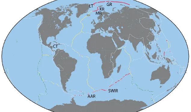
Figure 1.2. . The global ridge system. In grey are the global plate boundaries; in green the fast spreading ridges (spreading rate of 80-100 mm/yr); in red the ultraslow spreading ridges (spreading rate lower than 20 mm/yr); and in yellow all the other ridge segments. GR = Gakkel ridge, IT = lena trough, KR = Knipovich ridge, MR = Mohns ridge, CT = Cayman trough, AAR = America-Antarctic ridge, and SWIR = Southwest Indian ridge. (Snow and Edmonds, 2007)

(10)

10

2500 m and rough rift mountain topography weakly correlated to spreading rate. The morphology tends to be dominated by tectonic force (Dick et al. 2003). 4) Ultraslow spreading ridges.

Ultraslow spreading ridges include the Southwest Indian Ridge, the Gakkel Ridge and several smaller ridges. They are mainly sited at the poles with a total length of 15000 km, representing about 25% of the global mid ocean ridge system (Solomon, 1989). This ridge class is characterized by spreading rate of <20 mm/year and a thin oceanic crust (1-4 km) (Snow and Edmonds, 2007). The morphology of this ridge is similar of that of slow spreading ridge: high valley walls and rugged rift mountains. The axis of ultraslow spreading ridge is constituted by both magmatic and amagmatic accretionary ridge segments and they are linked together to make up a “supersegment”. In faster systems there are mainly magmatic segments that are linked together between transform faults to build first-order segments. In these systems transform faults are not present and are replaced by amagmatic accretionary ridge segments that are key component of ultraslow spreading ridges. Contrary to magmatic segments, they can assume any orientation relative to the spreading direction (Dick et al. 2003).

Extensive outcrops of serpentinized peridotites are exposed in the crust of these systems (Cannat et al., 2010), due to prevalence of tectonic processes that lead the uplift and exposure of material from upper mantle and lower crust. This material, low-silica ultramafic rocks (mainly olivine and pyroxene), undergoes water-rock reactions (Schrenk et al., 2013). The result is the oxidation of ferrous iron from olivine and pyroxene, the precipitation of ferric iron in magnetite and other minerals and the release of diatomic hydrogen. The combination of diatomic hydrogen and carbon dioxide or carbon oxide under highly reducing conditions

(11)

11 leads to formation of methane (Charlou et al., 2010). These reactions are highly exothermic and contribute significantly to the overall hydrothermal fluxes (Früh-Green et al. 2003). These fluxes provide reduced energy to the system and develop a diffused dissipation of the heat from the lithosphere (Dick et al. 2003). Another factor that could lead to a heat diffused system is the low thickness of the crust, due to the proximity of hot mantle to seawater and sediments. All these aspects could have a strong impact on generation of hydrothermal circulation and therefore on the structure of the microbial community, whose structure could be influenced (e.g. less chemolithotrophs) if a minor input of reduced molecules occurs as result of diffused input of hydrothermal fluids (Kelley et al., 2007). Habitats that have characteristics similar to ultramafic systems are seep systems. Here the leakage of heat is widespread like in ultramafic systems and the fluid have a similar composition, being rich in methane and poor of reduced metals (Hovland et al., 2012).

In 1990s a linear relationship between the spreading rate and hydrothermal activities was proposed (Baker et al., 1996). Because of the very slow spreading rate of these ridges they were supposed to be inactive and without any hydrothermal activity. Furthermore, their geographical position (mainly the poles) didn’t allow the study of this class of ridge until a development of research devices (German et al., 2010). Afterwards, the ultraslow spreading ridge was supposed to have only tectonic activities because the magma supply was supposed to be insufficient to support significant convection (Edmonds, 2010). First indirect evidence of the presence of hydrothermal venting in ultraslow spreading ridges was obtained in 1997 through a survey of water anomalies in SWIR (German et al., 1998). The first hydrothermal plume was detected during at the R/V Knorr

(12)

12

Cruise 162 in segment 10 and 16°E of SWIR (Bach et al., 2002). Another evidence of hydrothermal activity in this system was obtained in 2007 during the Chinese research cruise DY115-19 (Tao et al., 2012). At the Gakkel Ridge, evidences of hydrothermal activity where found in 2003 during the AMORE cruise, and in 2008 during an International Polar Year expedition pyroclastic deposits with fragmented magma were found (Sohn et al., 2008). All these works support the hypothesis that high temperature hydrothermal circulation is widespread along all ultraslow spreading ridges despite the low magma supply.

1.4 South West Indian Ridge

Southwest Indian Ridge (SWIR) extends between the Rodrigues Triple Point in the southern Indian Ocean and the Bouvet Triple Junction in the south Atlantic, so it represents the only way for chemosynthetic deep sea vent fauna for their dispersion between Atlantic and Pacific ridge systems (Baker at al., 2004). The vent fields may provide suitable “stepping stone” niche environments that can sustain chemosynthetic ecosystems and enhance the flow among different systems. During the ChEss programme, whose aim was an improving of the knowledge of the biogeography of deep water chemosynthetically driven systems, it was observed as vent species along the Southeast Indian Ridge showed increasing influence of Pacific faunas, whereas along the Southwest Indian Ridge, Atlantic influences were greater (Tyler et al., 2003). However, due to few studies describing the hydrothermal communities at SWIR (Peng et al, 2011), there are weak evidences in support of this observation.

The SWIR can be divided into a number of subsections based on changes in the obliquity of the ridge axis and on the variation of regional axial depth. As obliquity increase, the spreading rate slows proportionally (Tao et al., 2012). The average

(13)

13 speed of SWIR is almost 14 mm/year but we can find several segments with different speed; in the work of Dick et al. (2003) this ridge is defined as a transitional system between slow and ultraslow spreading ridge.

The SWIR segment, which I deal in my thesis, extends between 10°-16°E. The average depth is 4000 m and extended peridotite outcrops in the ridge axis are present. This area has the slowest spreading rate of any other oceanic ridge (8.4 mm/year); this peculiar characteristic is due to its very oblique orientation (51° from the spreading direction; Dick et al., 2003). Here, during the R/V Knorr Cruise 162, evidences of two active vent sites, massive sulfide deposits, sepiolite deposits, silica deposits and Mn-oxide breccias were revealed. This discovery is remarkable because it proves that the presence of hydrothermal material and activity is not strictly connected with magma supply rate and mantle upwelling, as along this section they are lower than on any other studied ridge segments. Therefore, the presence of hydrothermal activity in this area could reflect a tectonic control on fluid circulation (Bach at al., 2002), and contribute to dispersion route for the hydrothermal fauna.

(14)

14

2. Objectives

In 2013 along the segment 10°-16° E of the South West Indian Ridge a multidisciplinary survey, involving seismologic, geologic, microbiological analyses, was carried out during the expedition ANTXXIX/8.

Sediment sampling was focused on selected target sites that were characterized by anomalies in water column, situated in fault systems or showed high heat flux. No hydrothermal plumes or black smoker systems were found in this area. However, high heat flux was measured in one station, and in another station sediment enriched in reduced compounds was collected and the presence of vent fauna were reported by photographic survey. All these aspects suggest that a hydrothermal circulation was present in this investigated SWIR segment. Thus if this hydrothermalism is associated to fluid emissions then benthic organisms should be influenced in some extent.

The aim of my work is to provide a biological evidence of the presence of hydrothermal circulation in this area, as no previous microbial studies have been conducted in this segment. In my study, I hypothesized that a difference in the microbial community structure is present amongst areas that show different geochemical characteristics and in particular, I expect to find a microbial community related to those isolated from hydrothermal-driven systems in the area where high reduced molecules and hydrothermal fauna have been observed.

(15)

15

3. Materials and Methods

3.1 Sample collection

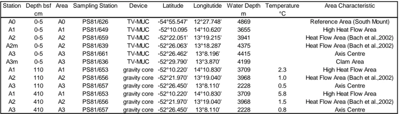
The samples were collected during the expedition ANTXXIX/8 between November and December 2013 in the segment 10°-16°E of the Southwest Indian Ridge (SWIR), with R/V POLARSTERN. Sediment samples have been taken from seabed at depth range of 2228 and 4869 m. Superficial sediment samples, the first 30-40 cm, have been collected with multi corers device (MUC) and subsurface samples, from 1 m below seafloor (bsf) up to 6 m bsf, with a gravity core (GC). All sampled sediments were stored at -80° C. I investigated sediments sampled in one reference station, located outside and south of the rift valley, and 5 stations inside the valley (Figure 3.1). I analysed one sediment layer, 0-5 cm bsf, in the reference area and three different layers in areas situated inside the ridge valley: 0-5 cm, 110 cm and 410 cm bsf (Table 3.1). These layers have been selected according to geochemical profiles (Figure 3.2).

Figure 3.1. Map of study areas; a) SWIR area and the reference station (A0); b) the location of the study stations inside the SWIR area.

(16)

16

3.2 Area Characterisation

During RV POLARSTERN cruise P81 to the SWIR, an integrated study was carried out employing seismology, geology, microbiology, deep-sea ecology, heat flow and others. The objectives of this expedition were to confirm the presence of hydrothermal circulation, hypothesized by earlier study (Bach et al., 2002), and to identify and localize the origin of hydrothermal plume.

The data collected on field did not provide evidence of temperature, redox potential and turbidity anomalies in water column, usually applied like a proxy for hydrothermal plume signature, as previously described by Bach and colleagues (2002), as well as vigorous fluid flow in the form of black smokers or shimmering water could not be observed at seafloor. However enhanced heat flow due to upward pore water migration was measured. This leads to values of very high heat flow (up to 850 mW/m2_{) and advection rates up to 25 cm/s. Enhanced}

biomass and a greater variation of megafauna along those sites of high heat flow could be inferred from reconnaissance observations with a camera sledge. A closer investigation of microbial activity in the material of gravity corers revealed favorable living conditions for microorganisms. Furthermore in few stations chemosynthetic fauna, typical of deep-sea hydrothermal habitats such as clams and worms, has been collected.

Table 3.1. Description of stations here investigated.

Station Depth bsf Area Sampling Station Device Latitude Longitutide Water Depth Temperature Area Characteristic

cm m °C

A0 0-5 A0 PS81/626 TV-MUC -54°55.547' 12°27.748' 4869 Reference Area (South Mount) A1 0-5 A1 PS81/649 TV-MUC -52°10.095 14°10.620' 3655 High Heat Flow Area A2 0-5 A2 PS81/659 TV-MUC -52°22.051' 13°19.215' 3941 Heat Flow Area (Bach et al.,2002) A2m 0-5 A2 PS81/639 TV-MUC -52°26.063' 13°18.287 4375 Heat Flow Area (Bach et al.,2002)

A3 0-5 A3 PS81/661 TV-MUC -52°26.462' 13°8.196' 4415 Axis Centre A3m 0-5 A3 PS81/636 TV-MUC -52°29.790' 13°3.870' 4199 Clam Area

A1 110 A1 PS81/653 gravity core -52°10.220' 14°10.830' 3709 2.3 High Heat Flow Area A2 110 A2 PS81/656 gravity core -52°21.970' 13°19.040' 3968 1.0 Heat Flow Area (Bach et al.,2002) A3 110 A3 PS81/657 gravity core -52°26.450' 13°8.110' 2228 0.5 Axis Centre A1 410 A1 PS81/653 gravity core -52°10.220' 14°10.830' 3709 5.8 High Heat Flow Area A2 410 A2 PS81/656 gravity core -52°21.970' 13°19.040' 3968 1.5 Heat Flow Area (Bach et al.,2002) A3 410 A3 PS81/657 gravity core -52°26.450' 13°8.110' 2228 0.8 Axis Centre

(17)

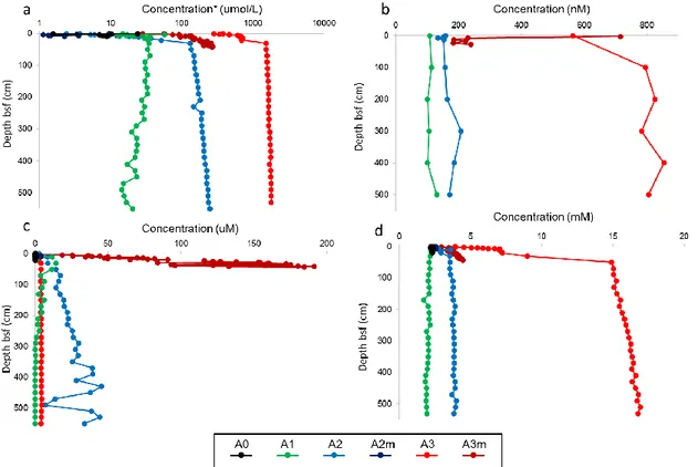
17 The geochemical analysis of pore water extracted both from MUC and GC sediments showed interesting differences between stations inside the valley and the reference station. In particular anomalies and upward decreasing in concentration of ammonia, methane, sulfide and dissolved inorganic carbon (DIC) suggest the presence of hydrothermal emissions in western area of SWIR’s segment investigated (Figure 3.2).

According with these preliminary results the sampling stations were grouped into four areas with different characteristics: 1) area 0 (A0): reference station located outside and south of SWIR; 2) area 1 (A1): higher heat flow; 3) area 2 (A2): sites were plume signature were reported in previous study; 4) area 3 (A3): sites with geochemical anomalies in pore water and where chemosynthetic fauna (e.g. Vesycomid clam) has been retrieved.

Figure 3.2. Geochemical sedimentary profiles for MUC and gravity core samples: a) Ammonium; b) Methane; c) Sulphide; d) DIC. * Logarithmic scale.

(18)

18

3.3 DNA Extraction

In order to study the microbial community, DNA was extracted from different stations and layers of the four areas described above. I selected 6 samples of the layer 0-1 cm, 6 samples of the layer 1-5 cm, 4 samples of 110 cm and 4 samples of 410 cm (shown in Table S1). As the samples are constituted by different sediment typologies, and this can affect DNA extraction yield, I tested different extraction procedures in order to obtain similar DNA amount and quality from all areas. The following DNA extraction kits were tested: UltraCleanTM_{Soil DNA}

Isolation Kit (MoBio laboratories Inc.), FastDNATM_{SPIN Kit for Soil (Q-BIOgene),}

PowerSoilTM_{DNA Isolation Kit (MoBio laboratories Inc.). All the extractions were}

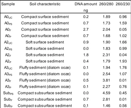
performed following the manual protocols. I selected four different samples according with sediment tipology: A0, A2, A3 and one subsurface sample (soil characteristics shown in Table 3.2). I extracted DNA from 0.5 g of sediment from each sample. After each extraction, DNA concentrations and DNA quality, measured as 260/280 (it indicates the purity of DNA and RNA; a ratio of about 1.8 indicates “pure” DNA) and 260/230 ratio (it indicates the nucleic acid purity; the ratio is normally in the range of 2.0-2.2), have been quantified with NanoDrop (Thermo SCIENTIFIC 1000). As shown in Table 3.2, the higher amount of DNA was obtained with FastDNATM_{SPIN Kit for Soil but with this method, the lower}

quality of DNA was obtained. This could be due to presence of humic acids in the sediments (Tebbe and Vahjen, 1993); in order to remove these compounds, I performed a DNA precipitation on samples extracted with FastDNATM_{SPIN Kit}

for Soil (Table 3.2). Precipitation was executed in ethyl acetate and isopropanol. After the addition of an amount of ethyl acetate (7.5 M) equal to 1/3 of the sample volume and of an amount of isopropanol equal to the volume of the sample, DNA

(19)

19 was incubated overnight at -20 °C. Then a centrifugation was performed to allow the DNA precipitation and the removal of the supernatant. DNA was suspended in ethanol 70% in order to clean again the DNA. The solution was centrifuged again and the ethanol was removed. The last suspension was made with TE buffer. All the DNA samples were stored at -20°C.

Furthermore, I tested the amplificabily of the 16S segment of the extracted DNA, performing a PCR (Polymerase Chain Reaction). The amplifications were carried out in 20-μl reaction mixtures that consisted of 1 μl of DNA template, 1.5 mM 10× PCR buffer (Mg++), 200 μM deoxynucleoside triphosphate, 0.5 μM concentrations of each primer, 0.0125 U/μl of Taq DNA polymerase. In order to amplify nearly full length 16S rRNA, I used universal bacterial primers GM3F and GM4R (5'-AGAGTTTGATCMTGGC-3' and 5'-TACCTTGTTACGACTT-3'); and archaeal universal primers 20F (5‘-TTCCGGTTGATCCYGCCRG-3‘) and 1492R (5'-TACGGYTACCTTGTTACGACTT-3‘). 20 ul of DNA from each sample was

Table 3.2. Results of DNA extractions carried out with different extraction kits. UC, samples extracted with

the UltraCleanTM_{Soil DNA Isolation Kit; F, FastDNA}TM_{SPIN Kit for Soil; PS, PowerSoil}TM_{DNA Isolation Kit;}

P, FastDNATM_{SPIN Kit for Soil followed by precipitation. Sub, subsurface sample. 260/280 and 260/230}

are ratios that indicate the purity of the DNA: a 260/280 ratio of about 1.8 indicates “pure” DNA and 260/230 ratio indicates a good nucleic acid purity if it is in the range of 2.0-2.2.

Sample Soil characteristic DNA amount 260/280 260/230 ng

A0UC Compact surface sediment 0.2 1.89 0.96

A0PS Compact surface sediment 0.7 1.73 1.59

A0F Compact surface sediment 2.7 2.04 0.05

A0P Compact surface sediment 0.7 1.68 1.02

A2UC Soft surface sediment 0.9 1.90 1.66

A2PS Soft surface sediment 0.0 1.83 0.99

A2F Soft surface sediment 1.8 2.31 0.04

A2P Soft surface sediment 0.4 1.79 1.93

A3UC Fluffy sediment (diatom ooze) 0.1 1.94 1.76

A3PS Fluffy sediment (diatom ooze) 0.0 2.54 1.07

A3F Fluffy sediment (diatom ooze) 0.5 3.81 0.01

A3P Fluffy sediment (diatom ooze) 0.1 2.27 0.76

SubPS Compact subsurface sediment 0.0 4.59 0.45

SubF Compact subsurface sediment 0.7 2.81 0.01

(20)

20

loaded in Thermal Cycler (ThermoFisher SCIENTIFIC): bacterial DNA was amplified for 30 cycles (1 min of denaturation at 95°C, 1.5 min of annealing at 44°C, and 3 min of elongation at 72°C); archaeal DNA was amplified for 30 cycles (1 min of denaturation at 95°C, 1 min of annealing at 55°C, and 2 min of elongation at 72°C). The electrophoresis was performed on agarose gel (1%); in order to control the reliability of PCR, positive and negative controls were used. The gel was visualized under ultraviolet light after ethidium bromide bath. In Figure 3.3, it is shown as the better results were obtained with FastDNATM_SPIN

Kit for Soil.

FastDNATM_{SPIN Kit for Soil was selected to extract DNA from all the samples}

reported in the Table S1. The FastDNA extraction is not a chloroform phenol method; briefly the procedure followed these steps: i) the mechanical cell lysis is carried out by a mixture of ceramic and silica particles; ii) the addition of reagents permits to protect and solubilize nucleic acid upon cell lysis, minimize RNA contaminations, enhance the protein precipitation; iii) the addition of a DNA binding reagent allows the DNA holding; iv) the passage of DNA through a filter permits the holding of DNA at the filter (this passage has to be repeated 3-4 times); v) the DNA is eluted in pure PCR water and stored at -20°C. After every DNA extraction, DNA yield was measured.

The DNA concentrations of subsurface samples were lower than the surface sediment (Table S1), thus the subsurface DNA was precipitated and suspended in appropriate volume to have comparable concentration with surficial DNA (precipitation procedure is described above). Furthermore, in order to have comparable amount of DNA, I performed 2 extractions on surface samples and 4

(21)

21 extractions on subsurface samples. The DNA extracted from layers 0-1 cm and 1-5 cm was combined. A total of 2 g of sediment per samples were extracted from both surface and subsurface layers.

To verify that the extracted DNA was amplifiable, I performed PCR on all the extracted DNA samples (with the same procedure described above). I had some problems to amplify archaeal DNA, which were resolved changing annealing temperature, PCR reaction mixture and using a pair of primers that amplify a shorter fragment (958R [5’-CCGGCGTTGANTCCAATT-3‘] and 20F).

In the Table 3.3, the selected and shipped samples are shown; the Figure 3.4 shows PCR products on electrophoresis gel of these final samples.

Figure 3.3. Electrophoretic run in agarose gel (1%) for PCR products (amplified 16S segments) of DNA extracted with different kits; a)archaeal 16S; b)bacterial 16S. Highlighted in red are the DNA samples

(22)

22

Figure 3.4. Results of PCR for testing the 16S amplification of DNA for sequencing. a) bacterial samples; b) archaeal samples. La, low DNA Mass Ladder; PCb, Positive Bacterial Control; NCb, Negative bacterial Conrol; PCa, Positive Archaeal Control; NCa, Negative archaeal Control. In yellow are the 0-10 cm sediments; in orange the 110 cm sediments; in blue the 410 cm sediments.

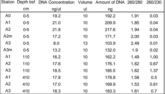
Table 3.3. Table that reports DNA concentrations, volume, amount and 260/280 and 260/230 ratios of DNA samples that were shipped for the amplification.

Station Depth bsf DNA Concentration Volume Amount of DNA 260/280 260/230

cm ng/ul ul ng A0 0-5 19.2 10 192.2 1.91 0.03 A1 0-5 21.0 10 209.9 1.85 0.04 A2 0-5 21.8 10 217.6 1.94 0.04 A2m 0-5 17.2 10 171.7 2,00 0.03 A3 0-5 8.0 13 103.9 2.49 0.01 A3m 0-5 13.2 10 132.0 1.9 0.02 A1 110 16.2 10 162.2 1.49 1,00 A2 110 17.6 10 176.1 1.62 0.67 A3 110 18.5 10 185.5 1.62 1.37 A1 410 17.8 10 178.8 1.58 0.5 A2 410 17.0 10 169.9 1.53 0.61 A3 410 18.3 10 183.3 1.61 0.7

(23)

23

3.4 DNA Sequencing

The extracted DNA was shipped to CeBiTec laboratory (Centrum für Biotechnologie, Universität Bielefeld) and was sequenced with the Illumina MiSeq platform. For 16S amplicon library preparation we used bacterial primers 341F (5´-CCTACGGGNGGCWGCAG-3´) and 785R (5´-GACTACHVGGGTATC TAATCC-3´) and archaeal primers Arch349F (5´-GYGCASCAGKCGMGAAW-3´) and Arch915R (5´-GTGCTCCCCCGCCAATTCCT-3´), which amplified 16S region V3-V4 for Bacteria (length fragment 420 bp) and V4-V6 for Archaea (length fragment 510 bp).

The amplicon library was sequenced with the MiSeq v3 chemistry, in a 2x300 bases paired device. The Illumina sequencing mechanism is, briefly: i) short DNA sequences (adaptors) are attached to the DNA fragments; ii) DNA segments are denatured with sodium hydroxide, and made single stranded; iii) once prepared, the DNA fragments are washed across the flowcell and the complementary DNA binds to primers on the surface of the flowcell whereas the DNA that doesn’t attach is washed away; iv) the DNA attached to the flowcell is replicated to form clusters of DNA with the same sequence; these clusters have to be big enough to emit a strong signal that will be detected by a camera; v) unlabelled nucleotide bases and DNA polymerase are added to extend and join the strands of DNA attached to the flowcell. This creates ‘bridges’ of double-stranded DNA between the primers on the flowcell surface; the double-stranded DNA is then denatured into single-stranded DNA using heat, leaving several million dense clusters of identical DNA sequences; vi) primers and fluorescent labelled terminators, nucleotide bases that stop DNA synthesis, are added to the flowcell; vii) the primer attaches to the DNA being sequenced, vii) the DNA polymerase then binds

(24)

24

to the primer and adds the first fluorescently-labelled terminator to the new DNA strand. Once a base has been added no more bases can be added to the strand of DNA until the terminator base is cut from the DNA; ix) lasers are passed over the flowcell to activate the fluorescent label on the nucleotide base; the fluorescence is detected by a camera and recorded on a computer; each of the terminator (different bases) emits in a different colour; x) the fluorescently-labelled terminator group is then removed from the first base and the next fluorescently-labelled terminator base can bind the DNA stand; this process continues until millions of clusters have been sequenced.

The output of the this sequencing are millions of reverse and forward reads that overlap for a variable number of base pairs, depending on the used primer; in our samples the overlap is about 40-80% for bacteria and about 30% for archaea. Thus the reverse and forward reads had to be merged before to analyze the sequencing date, as well as cleaning and quality control was carried out. The Table 3.4 reports the number of sequences before and after cleaning and merging. First, I removed the primers from the reads with the command-line tool cutadapt (Martin, 2011). Then I used the software TRIMMOMATIC (Bolger et al., 2015) in order to remove the sequences that did not have a good quality; this step has been performed before the reads merging for bacteria and after merging for archaea. The difference in the procedure is due to the different length of the segments (and consequently, the overlapped region between reverse and forward reads). The quality of the sequencing is usually lower at 3’-region of the reads (Bartram et al., 2011), so if there are long fragments, as I have for archaea, it is better performed the trimmomatic step after the merging because these could enhance the number of the holding reads. The merging step was performed with

(25)

25 the PEAR software (Zang et al. 2013). The operational taxonomic unit (OTU) clustering has been made with SWARM (Mahè et al. 2014). OTUs were built with a similarity threshold of 97%. I used this method because the clustering is low influenced by clustering parameters and products robust OTUs. The taxonomic classification is based on SILVA database (Quast et al., 2013). During this step, sequences with less than 90% of similarity with SILVA sequences have been removed; this removal was done in order to remove the presence of amplification and sequencing artifacts, as chimera; the weakness of this approach is the high probability to exclude unknown organisms.

3.5 Statistical analysis

All analyses were carried out in the R statistical environment (R Development Core Team, 2009) with the packages vegan (Oksanen et al., 2010) and ggplot2 (Wickham, 2009), as well as with custom R scripts.

The bacterial and archaeal communities of surface and subsurface sediments were analyzed separately. The number of singletons, doubletons and unique OTUs was calculated separately for surface and subsurface. Singletons (SSO)

a

A0 A1 A2 A2m A3 A3m A1 A2 A3 A1 A2 A3 Reads* 87522 123394 59037 55752 39162 54320 169752 159425 92251 48417 115178 146723 Clipped reads* 83590 118163 56328 53224 37440 51852 162567 152438 88613 46317 110355 140707 Trimmed reads* 83558 118126 56312 53195 37431 51833 162498 152383 88574 46295 110324 140663 Assembled reads 82921 117610 56083 52985 37130 51583 161040 151510 88019 45941 109743 139931

b

A0 A1 A2 A2m A3 A3m A1 A2 A3 A1 A2 A3 Reads* 51982 57240 52121 59126 52415 96761 58347 63821 52467 59727 52298 50405 Clipped reads* 32171 39895 33848 38961 40481 71740 46766 44516 41141 49139 37144 38872 Assembled reads 27023 33308 28817 33633 30577 58977 27556 31290 30787 32840 28368 30339 Trimmed reads 3666 3464 3657 6502 10456 11691 2466 5104 3711 4833 2528 4901 0-5 110 410 0-5 110 410

Table 3.4. Table with number of reads after every steps of the quality cleaning. *these numbers represent only the reverse or forward reads, as these steps were performed before the reads merging.

(26)

26

are defined as the OTUs that are represented with one sequence in the entire dataset; doubletons (DSO) are the OTUs that are presents with two sequences in only one sample; and unique OTU (OTUunique) are OTUs that are present only

in one samples but with more than 2 sequences. With absolute percentage (SSOabs, DSOabs and OTU unique abs) I refer to number of singletons, doubletons

and unique OTUs present in a sample relative to total number of OTUs of the surface or subsurface dataset, whereas with relative percentage (SSOrel) I refer

to the contribution of singletons present in a certain sample to total number of OTUs for that sample.

Inverse Simpson (InvS), Exponential Shannon (ExpS), and Chao1 were calculated on a subsampled community to minimize the influence of errors due to the DNA amplification and sequencing. Subsampling was performed randomly taking in consideration the minor number of sequences (30826 for Bacteria and 2073 for Archaea). In order to assess if the subsampling invalidated Chao1, ExpS, InvS indexes and the nOTU, Mantel tests were performed on Eucliden matrixes calculated on those indexes values (calculated with and without subsampling). Furthermore, to calculate if the community structure (CS) between subsampled and not sampled dataset changed, Mantel test was performed on a Bray-Curtis dissimilarity matrix.

To study the diversity between different samples, beta diversity was calculated applying Jaccard index on OTUs presence/absence matrix. Thus the beta-diversity is here a OTUs turnover, showing the number of OTUs shared amongst samples.

The other analyses where performed on the dominant community, here defined as the community without the presence of singletons. Non-metric

(27)

27 multidimensional scaling (nMDS) scatterplots have been performed with average method at OTUs and every taxa levels in order to visualize the main clusters and patterns of the dataset.

Similarity Percentages (SIMPER) analysis was performed on OTU dataset to identify the main OTUs responsible of differences observed in nMDS plot. As the SIMPER analysis tends to underlines the most abundant objects that are responsible for the observed dissimilarity, an in-depth analysis of the dataset was performed in order to detect all the interesting taxa. Particular importance was given to those taxa that were exclusively, or mainly present in A3 or that showed a decrease abundance from A3 to A0. In addition, in order to have results less biased as possible, I inspected taxa that showed highest relative abundances in A0.

Taxa analyses were carried out with BLAST software (Camacho et al., 2009) and the construction of phylogenetic trees.

3.6 Phylogenetic Tree’s Construction

The phylogenetic trees were constructed with Arb software (Ludwig et al., 2004) for those taxa that were highlighted by SIMPER or that showed important changes in relative abundance between areas. The aim of my phylogenetic trees was to see where the prokaryotes more phylogenetically related to my sequences where isolated and if metabolic information were available. The latter is a critical issue, since microbial community of deep sea ecosystems are barely studied and really few organisms have already been cultured (Sogin et al., 2006) so metabolic information were not present for the majority of taxa present in my dataset. First, the sequences of the studied taxon were aligned with SINA aligner (Pruesse et al., 2012); then they were added to the Silva tree with Parsimony method.

(28)

28

Closest reference sequences were selected and used to build a new tree with Maximum Likelihood method with bootstrap statistical analysis (500 repetitions); the used software was RAxML 8 (Stamatakis, 2014).

Once, constructed the tree backbone with the referenced sequences, my sequences were added with Parsimony method, without any change in the tree topology.

I applied this procedure because the Illumina 16S tag sequencing produces sequences too short (<550 bp) to allow the construction of a solid backbone tree, which, for this reason, was built using only 16S segments longer than 900 bp. Furthermore, because the taxonomy of the family DHVEG-6 changed recently (Eme and Doolittle, 2015), for this archaeal family I choose to build a second phylogenetic tree. The procedure for the construction of this tree has been the same but, as reference sequences, I selected only organisms previously cultured (Castelle et al., 2005). This approach allowed to better inferring about potential metabolism of OTUs belonging this taxon.

The phylogenetic trees were ultimate in the R statistical environment (R Development Core Team, 2009) with the packages phyloseq (McMurdie and Holmes, 2014), ade (Paradis et al., 2004), ggplot2 (Wickham, 2009), stringi (Gagolewski and Tartanus, 2015) and plyr (Hadley, 2011).

(29)

29

4. Results

Since the rare biosphere (i.e. singletons) represented the large fraction of total OTUs and the number of sequences recovered showed an high variability between samples (Table 4.1; Table 4.2), thus subsampling of Illumina sequences was performed in order to normalize the dataset and therefore to have a better comparison of alpha-diversity between samples.

Mantel test, showing a high correlation between alpha-diversity indexes and community composition calculated on the whole dataset and the subsampling dataset (Table 4.3), highlighted that the bacterial and archaeal diversity and community structure in the subsampling dataset reflected the patterns observed for whole dataset. For this reason, differences in bacterial and archaeal community composition were analysed on whole dataset. Furthermore the rare biosphere (i.e. the singleton component) was not taken into account for analysis of differences in community composition. Conversely, to be conservative, in the following section I described the OTU richness (number of OUTs) for whole dataset and diversity indices (i.e. Chao1, Exponential-Shannon and Inverse-Simpson) for subsampled dataset. Instead sequence number (nSeq), single-sequence OTU or singleton (SSO), double-single-sequence OUT or doubleton (DSO) and unique OTU (OTUunique) were referred to whole dataset.

4.1 Bacterial Diversity

4.1.1 Comparison between surface and subsurface

The sequencing dataset showed a variable number of sequences amongst different samples (Table 4.1). In general, the sequence number was higher in subsurface samples than in surface samples.

(30)

30

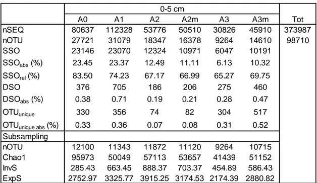
Table 4.1. Description of bacterial number of sequences, richness, alpha-diversity and rare biosphere at each site. a) surface layers; b) subsurface layers. nSEQ, total number of sequences; nOTU, number of

OTUs; SSO, number of singletons; SSOabs, percentage of singletons relative to total number of OTUs;

SSOrel, percentage of singletons relative to number of OTUs of each sample; DSO, number of doubletons;

DSOabs, percentage of doubletons relative the total number of OTUs; OTUunique, number of unique OTU;

OTUunique abs: percentage of unique OTUs relative to total number of OTUs. InvS, Inverse Simpson index;

ExpS, exponential Shannon index. Subsampling was performed using the minimum bacterial sequences value (30826).

a

A0 A1 A2 A2m A3 A3m Tot

nSEQ 80637 112328 53776 50510 30826 45910 373987 nOTU 27721 31079 18347 16378 9264 14610 98710 SSO 23146 23070 12324 10971 6047 10191 SSOabs (%) 23.45 23.37 12.49 11.11 6.13 10.32 SSOrel (%) 83.50 74.23 67.17 66.99 65.27 69.75 DSO 376 705 186 206 275 460 DSOabs (%) 0.38 0.71 0.19 0.21 0.28 0.47 OTUunique 330 356 74 82 304 517

OTUunique abs (%) 0.33 0.36 0.07 0.08 0.31 0.52

Subsampling nOTU 12100 11343 11872 11120 9264 10715 Chao1 95973 50049 57113 53657 41439 51152 InvS 285.43 663.45 888.37 703.37 454.89 586.43 ExpS 2752.97 3325.77 3915.25 3174.53 2174.39 2880.82

b

110 cm 410 cm A1 A2 A3 A1 A2 A3 Tot nSEQ 145953 141502 78211 41852 104178 126448 638144 nOTU 24732 23900 13264 11710 19929 21861 104839 SSO 21545 19504 10178 9163 16771 18137 SSOabs (%) 20.55 18.60 9.71 8.74 16.00 17.30 SSOrel (%) 87.11 81.61 76.73 78.25 84.15 82.97 DSO 291 410 230 123 202 387 DSOabs (%) 0.28 0.39 0.22 0.12 0.19 0.37 OTUunique 971 609 208 98 241 344

OTUunique abs (%) 0.93 0.58 0.20 0.09 0.23 0.33

Subsampling nOTU 6724 6982 6257 9027 7082 6761 Chao1 42112 34914 34929 74467 50125 41660 InvS 92.63 64.61 55.25 113.34 38.02 47.26 ExpS 653.12 610.01 459.22 1058.43 517.80 478.38 0-5 cm

(31)

31

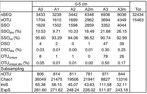
Table 4.2. Description of archaeal number of sequences, richness, alpha-diversity and rare biosphere at each site. a) surface layers; b) subsurface layers. nSEQ, total number of sequences; nOTU, number

of OTUs; SSO, number of singletons; SSOabs, percentage of singletons relative to total number of

OTUs; SSOrel, percentage of singletons relative to number of OTUs of each sample; DSO, number of

doubletons; DSOabs, percentage of doubletons relative the total number of OTUs; OTUunique, number of

unique OTU; OTUunique abs: percentage of unique OTUs relative to total number of OTUs. InvS, Inverse

Simpson index; ExpS, exponential Shannon index. Subsampling was performed using the minimum bacterial sequences value (2073).

a

A0 A1 A2 A2m A3 A3m Tot

nSEQ 3433 3239 3442 6348 6936 9036 32434 nOTU 1704 1610 1699 2962 3694 4349 15463 SSO 1629 1502 1598 2859 3352 4044 SSO_abs (%) 10.53 9.71 10.33 18.49 21.68 26.15 SSO_rel (%) 95.60 93.29 94.06 96.52 90.74 92.99 DSO 4 2 0 1 47 39 DSO_abs (%) 0.03 0.01 0.00 0.01 0.30 0.25 OTU_unique 8 1 1 0 78 26

OTUunique abs (%) 0.05 0.01 0.01 0.00 0.50 0.17

Subsampling nOTU 806 814 811 781 971 844 Chao1 36049 21475 19506 21941 8827 13316 InvS 65.38 56.15 45.07 43.63 111.58 32.11 ExpS 261.60 271.62 248.24 226.02 511.97 243.18

b

110 cm 410 cm A1 A2 A3 A1 A2 A3 Tot nSEQ 1565 3257 2746 3345 2073 4115 17101 nOTU 1058 1716 1646 1802 1133 1715 8724 SSO 986 1617 1556 1677 1053 1608 SSO_abs (%) 11.30 18.54 17.84 19.22 12.07 18.43 SSO_rel (%) 93.19 94.23 94.53 93.06 92.94 93.76 DSO 4 9 5 14 1 9 DSO_abs (%) 0.05 0.10 0.06 0.16 0.01 0.10 OTU_unique 3 14 5 9 1 8

OTU_{unique abs}(%) 0.03 0.16 0.06 0.10 0.01 0.09 Subsampling nOTU 1058 857 964 885 865 691 Chao1 30676 20666 27118 20308 32725 14960 InvS 141.13 54.00 59.03 64.56 43.46 23.53 ExpS 540.37 282.16 363.67 347.93 270.97 142.59 0-5 cm

(32)

32

The lowest number of sequences was found in the superficial sample A3 (30826 sequences) and the highest value was shown in the sample A1 (145953 sequences), collected at 410 cm bsf. The number of OTUs was also variable between samples, with maximum value at the surface sample A1 (31079 OTUs) and the minimum value at the surface sample A3 (9264 OTUs). The singleton percentages per sample (SSOrel) were higher in subsurface, ranged between

76% and 87%, than in surface samples, ranged between 65% and 83%. Lowest Chao1 was found at 110 cm in all areas (ranged between 34914 and 42112), and the highest values were described for deeper subsurface layer in A1 (74467); superficial samples ranged between 41439 and 57113. Inverse-Simpson (InvS) and Exponential-Shannon (ExpS) indexes are higher in superficial samples (455-888 and 2174-3915 respectively) than subsurface ones (38-113 and 459-1058).

4.1.2 Comparison between areas: surface

The maximum number of sequences and OTUs was found in A1 (112328 and 31079, respectively), whereas the lower values were observed in A3 (30826 and 9264, respectively). The number and relative abundance of singletons decreased from A0 (23146 and 23%, respectively) to A3 (6047-10191 and 6-10%, respectively). The expected richness (Chao1) was higher in A0 than SWIR areas,

Table 4.3. Mantel test performed on bacterial and archaea entire datasets and subsampled dataset. Mantel test on CS (Community Structure) has been performed on Euclidean distances matrix calculated on Bray-Curtis dissimilarity matrix; whereas, Mantel tests on Chao1 index, ExpS (Exponential Shannon) index, InvS (InverseSimpson) index and nOTU (number of OTUs) have been performed on Euclidean distance matrixes. Test r p r p CS 0.96 0.001 0.96 0.001 Chao1 0.96 0.001 0.98 0.001 ExpS 0.82 0.0005 0.95 0.001 InvS 0.86 0.001 0.67 0.014 nOTU 0.99 0.001 1.00 0.001 Bacteria Archaea

(33)

33 with lower richness in A3. InvS and ExpS indexes showed the lowest value in A0 and A3, and the highest in A2 (Table 4.1a).

4.1.3 Comparison between areas: subsurface

At 110 cm bsf we observed a decrease of the number of sequences and OTUs from area 1 to area 3, whereas an opposite trend was found for samples at 410 cm bsf. The SSOabs was highest at A1 for layer 110 cm (20%) and lowest at A1

for layer 410 cm (8%). Chao1, InvS and ExpS were higher in A1 than A2 and A3, in A1 these indices were higher at 410 cm than at 110 cm (Table 4.1b).

4.2 Bacterial Community Composition

The nMDS, performed on OTUs Bray-Curtis similarity matrix, showed two main clusters composed by surface and subsurface samples (Figure 4.1); samples inside these 2 groups had a dissimilarity values under the threshold of 90%. Considering a threshold of 80%, the two superficial A3 samples established a different cluster from the other surface samples; the same happens for the subsurface samples A1. With a dissimilarity threshold of 50% other clusters are formed: two superficial samples, A1 and control area, clustered separately; subsurface samples of Area 1 clustered separately from each other (Figure S1). nMDS performed at taxonomic levels (phylum, class, order, family and genus) showed similar clusters (data not shown). Analysing beta-diversity along the vertical profiles, the highest shared OTUs was between the two subsurface layers, and the value ranged between 15% and 39%. Values between surface and subsurface layers ranged between 0.4-6.5% (110 cm) and between 1.0-4.5% (410 cm). At A3, the number of shared OTUs along vertical profile was highest (6.5%, 39% and 4-4.5%, Figure 4.2c). Analysing horizontal surface profiles, the lowest beta-diversity value was observed amongst A3 other areas (5-14%).

(34)

34

Instead, in the subsurface layers the shared OTUs were higher between A2 and A3 (20%) than between A2 and A1 (13-18%; figure 4.2a).

4.2.1 Subsurface

The Figure 4.3 and Figure 4.4 show the relative abundance of the 10 most abundant families and classes per samples, respectively, and their patterns in areas investigated. At class level the differences between surface and subsurface community’s composition were mainly driven by dominance of Dehalococcoida, Candidate division OP8 and Candidate division JS1 in subsurface samples, whereas Gammaproteobacteria, Deltaproteobacteria, Alphaproteobacteria, Flavobacteria and Acidimicrobia were mostly present in superficial samples. The Candidate division JS1 increased from A1 to A3 in both layers, conversely Dehalococcoida and Candidate division OP8 did not show any consistent patterns between stations and layers. Interesting 9 OTUs belonging to JS1 and 16 OTUs belonging OP8 explained 25%, 25% and 27% of differences between

Figure 4.1 Multi-Dimensional Scaling (nMDS) plot performed on bacterial community with average method. The broken line indicates a dissimilarity threshold of 80%.

(35)

35

Figure 4.2. Diagram of beta-diversity amongst different stations and layers. Beta-diversity has been calculated applying dissimilarity Jaccard index on OTUs presence/absence matrix. a) bacterial beta-diversity along vertical profiles; b) archaeal beta-beta-diversity along vertical profiles; c) bacterial beta-beta-diversity along horizontal profiles; d) archaeal beta-diversity along horizontal profiles. Values in the brackets refer to A2m and A3m stations.

(36)

36

Figure 4.4. Plot representing the 10 most relative abundant bacterial classes in each sample. Figure 4.3. Plot representing the 10 most relative abundant bacterial families in each sample.

(37)

37 A3 and A1, between A2 and A1, and between A3 and A2, respectively (SIMPER; Table S2). Phylogenetic trees of JS1 and OP8 candidate division showed that these OTUs were phylogenetic related to bacterial clones found mainly in seeps, volcanoes and other subsurface ridges (Figure 4.5; Figure 4.6). The OTU55 and OTU105, belonging to the class Dehalococcoidia and explaining 0.8% of the differences between A3 and other areas, showed a higher relative abundance at A3 (2.4% and 1%, respectively) than at A2 and A1 (0.2% and 0.1%, respectively). However the BLAST alignment showed that only OTU105 was close related to Bacteria isolated from chemosynthetic environments (seep and mud volcano). Four OTUs (OTU77, 17OTU, 40OTU and 146OTU), belonging to Candidate Division KB1, had a relative abundance of 0.6%, 3.3% and 8.5%, respectively in A1, A2 and A3, and in phylogenetic tree they were clustered close to bacteria isolated from methane seeps (Figure 4.7).

4.2.2 Surface

The SIMPER highlighted that 25% of differences between surface community structure at A3 and those at other areas (A0, A1 and A2) were explained by 47 OTUs, 77 OTUs, and 88 OTUs, respectively, belonging to 49 different bacterial taxa (Table S3). Only for those OTUs whose relative abundance was higher at A3 than at A0, A1 and A2 the phylogenetic trees were constructed. The OTUs belonging to SEEP-SRB1 were present only in SWIR areas, and they were close related to bacteria isolated from deep-sea seeps, volcano and ridge habitats (Figure 4.8). In particular the OTU129 had a relative abundance of 0.2% and 1.8% at A3 and A3m, respectively, and explained 0.6-0.7% of differences in nMDS plots between A3 and other areas. The bacterial family JTB255 showed lowest relative abundance in A3 (Figure 4.3), however the relative abundance of

(38)

38

OUT187, belonging to not classified genus of JTB255, was higher at A3 (0.9-1.3%) than at A1 and A2, whereas it was not present A0, and it explained 0.7% of differences in bacterial community structure. The phylogenetic tree clustered this OTU close to bacteria isolated from ridge and hydrothermal systems (data not shown). The OTU224 belonging to bacterial class VC2.1 Bac22 showed a higher relative abundance in A3m (1.1%) than A3 (0.03%) and it was nearly absent in other areas. The phylogenetic tree showed this OTU clustered with an endosymbiont chemolithoautotrophic bacteria (Figure 4.9). The OTU170 and OTU101 belonging to Family SAR406 clade (Marine Group A) were dominant OTUs at A3 (1.6-1.7%, respectively) and explained 1.5-1.7% of differences between bacterial community at A3 and those at A0, A1 and A2. Closer related bacteria were found in marine sulfide deposit and ridge methane seeps (Figure 4.10). Furthermore, the OTU6369 and OTU6594 were found only in A3 surface samples (0.06% and 0.04% in A3 and A3m; respectively), and they were phylogenetically close to chemolithoautotroph bacterial clones. The differences in surficial bacterial community structure were also driven for 0.9-1% by OTU150 and OTU173 (family Anaerolineaceae), whom were present only at A3 (0.4-1%) and related bacteria were found in deep-sea methane and oil rich environments, and ridge fluids (data not shown). The Family Desulfarculaceae was found only in A3, representing 5.3% of bacterial community. In particular the OTU498 and OTU408, contributing to explain 0.3-0.4%, respectively, of SIMPER analysis, were clustered close to bacteria isolated from hydrothermal, mud volcano and oil polluted marine sediments (data not shown). The relative abundance of OTU402 and OTU794, belonging to phylum Candidate Division OP8, was 0.3% and 1.2% at A3 and A3m, respectively, and they were not found in other areas. They

(39)

39 explained 0.3-0.5% of difference in surficial community structure and were clustered close to bacteria isolated from deep-sea sediments and anaerobic methanotrophs isolated from mud-volcano (Figure 4.6). The OUT507, OTU599, OTU698 represented 1.3% of bacterial community at A3m, less than 0.1% in other SWIR areas, and they were not present in reference area. They belonged to family WCHB1-69, and they explained 0.3% of differences between areas. OTU507 and OTU698 clustered close to bacterial clones found in deep sea hydrothermal vent, terrestrial sulphide spring and hypersaline microbial mat. OTU599 clustered close to coral endosymbiont clones (data not shown). The OTUs belonging to subsurface phylum Candidate division JS1 (OTU48, OTU131 and OTU4) were only present in A3, with a relative abundance of 0.9-1.1%, and explained 0.7% of differences between bacterial communities. OTU131 and OTU48 clustered close to mud volcano and anoxic fjord bacterial clones; whereas OTU4 close to subsurface drilling sediment clones (Figure 4.5). Sulfurovum and Sulfurimonas (family Helicobacteraceae) were not selected by SIMPER, however they were exclusively present in A3, with highest relative abundance at A3m (0.9%). These genera include chemolithotrophic bacteria isolated from marine hydrothermal vents and cold seep systems (Figure 4.11).

The genus Spirochaeta showed an abundance of 1.3-1.5% in A3, whereas it is lower in the other areas. The phylogenetic tree showed that the OTUs, here found belonging to this genus, were related to systems of hydrothermal vents and methane seeps (data not shown). The genus Acidiferribacter showed a relative abundance of 0.6% and 0.2% in A3m and A3, respectively, and it was absent in A0; the analysis performed on BLAST platform highlighted its phylogenetic affinity to chemosynthetic organisms.

(40)

40

Furthermore, a crosscheck was carried out on OTUs that were highlighted by the SIMPER and that showed higher relative abundance in A0. The analysed taxa S085, Pseudomonas, Rubritalea, Candidate Division OM1 were found correlated with bacterial clones previously isolated from deep sea sediment.

4.3 Archaeal Diversity

4.3.1 Comparison between surface and subsurface

Superficial samples showed a higher number of sequences than subsurface samples, ranging between 3239-9036 and 1565-4115, respectively (Table 4.2). Number of OTUs showed a similar trend, with 1610-4349 OTUs in surficial samples and 1058-1802 in subsurface samples. The SSOrel was 91-96% and

93-95% for surficial and subsurface samples, respectively. The percentage of OTUunique was lower than 0.2% in all samples. Chao1 ranged between 8827 and

36049 in surface samples, and between 14960 and 32725 subseafloor layers. InvS showed values between 32 and 111 in surface layer and between 23 and 141 in subsurface layers. In surface samples, ExpS had a minimum value of 226 and a maximum value of 512, and it ranged between 143 and 540 in subsurface samples.

4.3.2 Comparison between areas: surface

The highest number of sequences and OTUs was observed in A3 (6936-9036 and 3694-4349, respectively) and in the sample A2m (6348 and 2962, respectively); in the other samples these values were less than 3500 sequences and 1800 OTUs. Highest SSOabs was observed in A3 and A3m (22% and 25%;

respectively); in other areas, this value ranged between 10% (A0, A1 and A2) and 18% (A2m). Highest Chao1 value was calculated for A0 (36050), inside the SWIR the estimated richness decreased from A1 to A3 (21475-8827). InvS and

(41)

41 ExpS decreased from A0 to A3m (65.4-32.1 and 162-243, respectively), however highest values were observed for A3 (111.6 and 512, respectively; Table 4.2a).

4.3.3 Comparison between areas: subsurface

In A1 and A3 the number of sequences and OTUs increased from 110 cm to 410 cm bsf, whereas an opposite trend was observed for A2. SSOabs didn’t show any

pattern between areas and layers; this value ranged between 11% and 19%. Chao1 didn´t show any consistent trend between areas and layers. InvS and ExpS were higher at A1 than at A2 and A3, and they decreased from 110 cm to 410 cm (bsf) in all areas (Table 4.2b).

4.4 Archaeal Community Composition

The NMDS plot showed that the A0 clustered separately from SWIR areas with a dissimilarity value of 70% (Figure 4.12). Considering a dissimilarity threshold of 60%, the superficial sample A3 clustered apart from the other samples. Whereas with the 40% of dissimilarity, four other clusters formed: A2 subsurface layers and A1 110 cm layer; A1 410 cm layer; both A3 subsurface layers and A3m surficial layer; A1 and A2 surficial layers (Figure S2).

Beta-diversity along vertical profile of A1 and A3, the surficial layer shared a major number of OUTs with deeper layer (410 cm) than with 110 cm. In A2 the number of OUTs shared between surficial layer and subseafloor layers decreased with sediment depth. In A2 and A3 the shared OTUs between subsurface layers were higher than those shared between surface layer and subsurface layers.

(42)

42

Conversely, in A1 the shared OTUs between subsurface layers were lower than those shared by surface and 410 cm layers (Figure 4.2d).

The analysis of surficial beta-diversity showed the same pattern observed for bacterial beta-diversity. I observed a lower number of shared OTUs between A2 and A3 than between A2 and A1, and a higher number of shared OTUs between A1 and A0 than between A1 and A3, with lowest OTUs shared between A3 and A0. In the 110 cm layer the beta-diversity decreased with distance between areas, conversely in 410 cm layer the number of shared OTUs between A2 and A3 was higher than between A2 and A1 (Figure 4.2b).

4.4.1 Surface and subsurface

At A0, the archaeal community was dominated by unclassified archaea belonging to Marine Group I and by Candidatus Nitrosopumilus (Figure 4.13). The latter dominated also in surficial and subsurface samples at SWIR areas, with exception for superficial station A3, where the dominant archaeal family was

Figure 4.12. Multi-Dimensional Scaling (nMDS) plot performed on archaeal community with average method. The broken line indicates a dissimilarity threshold of 70%.

(43)

43 Deep Sea Hydrothermal Vent Gp 6 (DHVEG-6; 53%). In subsurface layers other two important taxa were Marine Benthic Group D and Deep Sea Hydrothermal Vent Gp 1 (MBGD and DHVEG-1) and Group C3. The highest relative abundance of MBGD and DHVEG-1 was found in A1 (21% in the 110 cm layer and 16% in 410 cm layer); it was about 7% in A2 and 5% in A3. The relative abundance of C3 showed higher values in the deepest layer, here the value ranged between 9% and 12% in contrast with the 110 cm layer where the values ranged between 5% and 8%. Interesting phylogenetic tree showed that the majority of OTUs, belonging to DHVEG-6, clustered close to archaea isolated from hydrothermal and seep environments (Figure 4.14). Likewise, OTUs belonging to MBGD and DHVEG-1 were related to archaea identified in chemosynthetic environments (data not shown). The family Diapherotrites was found exclusively in surficial sediments of A3, and in particular the OTU47, representing 2.7% of archaeal community in the superficial sample of A3, was close to hydrothermal archaea in phylogenetic tree (data not shown). Five OTUs belonging to Marine Hydrothermal Vent Group (MHVG) were also found only at A3 (1.2%) and they were related to archaea described for chemosynthetic and methanogenic environments.

(44)

44

The phylogenetic tree of Marine Group I showed lack of differential OTUs clustering amongst investigated areas, with related archaea isolated both from deep-sea and hydrothermal systems (data not shown). Furthermore, I analysed OTUs belonging to the genus Candidatus Nitrosopumilus on the BLAST platform and, of particular concern is the OTU1 that was dominant at A3 (with a relative abundance of 27% in A3m), showed a decreasing trend from A2 to A0 (2%) and resulted phylogenetically close to methane-seep archaeal clones.

Figure 4.5. Phylogenetic tree of the phylum Candidate Division JS1. The tree backbone was constructed, including only the reference sequences, with Maximum Likelihood Method and 500 bootstraps were performed; then SWIR JS1 sequences were added with Parsimony Method. SWIR JS1 sequences are

(45)

(46)

(47)

47

Figure 4.6. Phylogenetic tree of the phylum Candidate Division OP8. The tree backbone was constructed, including only the reference sequences, with Maximum Likelihood Method and 500 bootstraps were performed; then SWIR OP8 sequences were added with Parsimony Method. SWIR OP8 sequences are bolded. Red writings indicate highlighted OTUs by the SIMPER.

(previous page)

Figure 4.7. Phylogenetic tree of the phylum Candidate Division KB1. The tree backbone was constructed, including only the reference sequences, with Maximum Likelihood Method and 500 bootstraps were performed; then SWIR KB1 sequences were added with Parsimony Method. SWIR KB1 sequences are bolded. Red writings indicate highlighted OTUs by the SIMPER.

(48)

48

Figure 4.8. Phylogenetic tree of the genus SEEP-srb1. The tree backbone was constructed, including only the reference sequences, with Maximum Likelihood Method and 500 bootstraps were performed; then SWIR SEEP-srb1 sequences were added with Parsimony Method. SWIR SEEP-SEEP-srb1 sequences are bolded. Red writings indicate highlighted OTUs by the SIMPER.

(49)

49

Figure 4.9. Phylogenetic tree of the order VC2.1 Bac22. The tree backbone was constructed, including only the reference sequences, with Maximum Likelihood Method and 500 bootstraps were performed; then SWIR VC2.1 Bac22 sequences were added with Parsimony Method. SWIR VC2.1 Bac22 sequences are bolded. Red writings indicate highlighted OTUs by the SIMPER.

Figure 4.10. Phylogenetic tree of the family Sar406. The tree backbone was constructed, including only the reference sequences, with Maximum Likelihood Method and 500 bootstraps were performed; then SWIR Sar406 sequences were added with Parsimony Method. SWIR Sar406 sequences are bolded. Red writings

(50)

(51)

51

Figure 4.11. Phylogenetic tree of the family Helicobacteraceae. The tree backbone was constructed, including only the reference sequences, with Maximum Likelihood Method and 500 bootstraps were performed; then SWIR Helicobacteraceae sequences were added with Parsimony Method. SWIR Helicobacteraceae sequences are bolded.

Figure 4.14. Phylogenetic tree of the archaeal family DHVEG-6. The tree backbone was constructed, including only the reference sequences, with Maximum Likelihood Method and 500 bootstraps were performed; then SWIR DHVEG-6 sequences were added with Parsimony Method. SWIR DHVEG-6

(52)