Geometric versus Model Predictive Control based guidance algorithms for fixed-wing UAVs in the presence of very strong wind fields.

Alma Mater Studiorum

University of Bologna

School of Engineering and Architecture

DEPARTMENT of ELECTRICAL, ELECTRONIC, AND INFORMATION ENGINEERING

"Guglielmo Marconi" - DEI

Master of Science in

Automation Engineering

Thesis in

Automatic Control

and System Theory

Geometric versus Model Predictive Control based

guidance algorithms for fixed-wing UAVs in the

presence of very strong wind fields.

Author:

Furieri Luca

Lecturer(s): Prof. Marconi Lorenzo (Univ. of Bologna) Prof. Siegwart Roland (ETH - Zurich) Supervisor(s): Ph.D. Stastny Thomas (ETHZ - Zurich) PostDoc. Gilitschenski Igor (ETHZ - Zurich)

Academic Year

2015/2016

Session

II

Contents

Abstract 3

Symbols 5

1 Introduction 1

2 A Nonlinear-Geometric Guidance Strategy to cope with

arbi-trarily strong windfields 3

2.1 Nonlinear guidance algorithms for fixed-wing UAVs: a brief review 3

2.1.1 Wind Compensation techniques . . . 5

2.2 Formal Problem Definition . . . 6

2.2.1 The Frenet-Serret framework for autonomous guidance . . 6

2.2.2 Feasibility Cone and Control Objective Formulation . . . . 9

2.2.3 The Nominal Solution in Absence of Wind in [1] . . . 11

2.3 The Lower Wind Case . . . 13

2.3.1 Previous solutions and their weaknesses . . . 13

2.3.2 Proposed strategy . . . 14

2.4 The Higher Wind Case . . . 18

2.4.1 Solution for ˆL0 feasible . . . 21

2.4.2 Infeasible desired direction: the state of the art. . . 21

2.4.3 Solution for ˆL0 infeasible . . . 22

2.5 Proof Of Stability . . . 25

2.5.1 Geometric case: finite paths . . . 25

2.5.2 Geometric case: infinite linear paths . . . 27

2.5.3 Dynamical case . . . 27 2.6 Continuity . . . 30 2.6.1 Sinusoidal Winds . . . 31 2.6.2 Rotating Winds . . . 31 2.7 Roll Dynamics . . . 34 2.8 Flight Results . . . 35 1

3.2 The MPC Guidance Approach For Fixed-wing Vehicles . . . 41

3.3 Simulation Results: A First Attempt . . . 43

3.4 Reshaping Of The Penalization Variable . . . 44

3.5 Simulation Results: Tackling Strong Winds . . . 46

4 Comparison Of Performance and Conclusions 49 4.1 Spatial Performance . . . 49

4.2 Conclusions . . . 52

4.3 Future Work . . . 53

Bibliography 57

Abstract

The recent years have witnessed increased development of small, autonomous fixed-wing Unmanned Aerial Vehicles (UAVs).

In order to unlock widespread applicability of these platforms, they need to be capable of operating under a variety of environmental conditions.

Due to their small size, low weight, and low speeds, they require the capability of coping with wind speeds that are approaching or even faster than the nominal airspeed.

In this thesis, a nonlinear-geometric guidance strategy is presented, addressing this problem. More broadly, a methodology is proposed for the high-level control of non-holonomic unicycle-like vehicles in the presence of strong flowfields (e.g. winds, underwater currents) which may outreach the maximum vehicle speed. The proposed strategy guarantees convergence to a safe and stable vehicle config-uration with respect to the flowfield, while preserving some tracking performance with respect to the target path.

As an alternative approach, an algorithm based on Model Predictive Control (MPC) is developed, and a comparison between advantages and disadvantages of both approaches is drawn.

Evaluations in simulations and a challenging real-world flight experiment in very windy conditions confirm the feasibility of the proposed guidance approach. Part of this abstract, Chapters 1 and 2 also appeared in [2] as a preprint, and were submitted for publication at ACC-2017, Seattle.

Symbols

Symbols

Indices

e east axis

n north axis

Acronyms and Abbreviations

ETH Eidgen¨ossische Technische Hochschule IMU Inertial Measurement Unit

UAV Unmanned Aerial Vehicle MPC Model Predictive Control

NMPC Nonlinear Model Predictive Control

NL NonLinear

LALE Low Altitude Long Endurance HIL Hardware In The Loop

Chapter 1

Introduction

In recent years, the use of small fixed-wing Unmanned Aerial Vehicles (UAVs) has steadily risen in a wide variety of applications due to increasing availability of open-source and user-friendly autopilots, e.g. Pixhawk Autopilot [3], and low-complexity operability, e.g. hand-launch.

Fixed-wing UAVs have particular merit in long-range and/or long-endurance re-mote sensing applications. Research in ETH Z¨urich’s Autonomous Systems Lab (ASL) has focused on Low-Altitude, Long-Endurance (LALE) solar-powered plat-forms capable of multi-day, payload-equipped flight [4], already demonstrating the utility of such small platforms in real-life humanitarian applications [5]. UAVs autonomously navigating large areas for long durations will inherently be exposed to a variety of environmental conditions, namely, high winds and gusts. With respect to larger and/or faster aircrafts, wind speeds rarely reach a signif-icant ratio of the vehicle airmass-relative speed. Conversely, wind speeds rising close to the vehicle maximum airspeed, and even surpassing it during gusts, is a frequent scenario when dealing with a small-sized, low-speed aircraft.

Usually in aeronautics, windfields are handled as an unknown low-frequency disturbance which may be dealt with either using robust control techniques, e.g. loop-shaping in low-level loops, or simply including integral action within guidance-level loops.

In the case of LALE vehicles, maximizing flight time would further require the efficient use of throttle, thus limiting airspeed bandwidth. In order to be able to use such systems safely and efficiently in a wide range of missions and di↵erent environments, it is necessary to take care of such situations directly at the guid-ance level of control, explicitly taking into account online wind estimates.

Goal of this thesis is to indeed develop guidance strategies that may cope with extreme wind-scenarios reliably and without the aircraft entering in emergency states.

Two di↵erent approaches will be explored. In chapter 2, a novel nonlinear-geometric guidance algorithm will be developed, building on some earlier results, in order to deal with arbitrarily strong and changing windfields. In chapter 3, we will develop a Model Predictive Controller that thanks to an underlying optimiza-tion procedure is able to automatically take care of the wind e↵ect. In chapter 4 the performances of the two approaches will be compared, and an attempt to draw conclusions about the main advantages and disadvantages of approaches will be made. Future extensions of this work will also be discussed in chapter 3.

Chapter 2

A Nonlinear-Geometric Guidance

Strategy to cope with arbitrarily

strong windfields

Throughout this chapter, a nonlinear-geometric approach for the guidance of small UAVs in strong windfields will be developed. First, a brief review of existing nonlinear guidance strategies and ways to take the wind into account will be provided in Section 2.1. Then the mathematical framework and the problem definition will be presented in Section 2.2, and the novel proposed nonlinear-geometric guidance strategy will be developed through sections 2.3, 2.4. A proof of stability in the case of higher winds will be provided in Section 2.5. Continuity properties of the algorithm to changing winds will be shown in Section 2.6. The behaviour of the algorithm when the actual roll-dynamics of real aircrafts are considered is analyzed in Section 2.7. The validation of the algorithm through real flight-tests will be presented in Section 2.8.

2.1

Nonlinear guidance algorithms for fixed-wing

UAVs: a brief review

Put simply, the goal of the guidance layer of control for UAVs is to make sure the vehicle will converge to and follow a given desired path. Though it should be noted there is a distinction between a path-following problem and a path-tracking problem, which is that in the path-following framework the path is defined spa-tially, while in the latter it is defined in the space-time domain (the vehicle is required to be in a certain place at a certain time) ([1]).

As in typical applications for small fixed UAVs it is required to cover certain areas to take images/perform patrolling task, we are most concerned about path-following: this is the problem we will consider throughout the chapter.

In [1], a point is made to remark that, ideally, the guidance layer of control for path-following is required to be simple to understand and implement, compu-tationally light for real-time flight, and as the path is defined geometrically it should not put constraints on the actual speed of the vehicle.

Additionally, as far as non-linear guidance algorithms are concerned, it is of pri-mary importance that the set of initial positions and velocities that allow to achieve convergence to the path is very large, if not infinite. In case this is not satisfied, it is required to switch between a manual-mode control and an automatic-mode control when the vehicle reaches a narrow neighbourhood of the path, which is far from being optimal in real applications ([1]).

Also note that many control-theoretic algorithms result in huge control inputs as the vehicle is far from the path (one could simply think of a PID controller, for example): this is another reason why the set of initial conditions might be severely restricted. This is why a generalized law allowing to perform completely autonomous flight starting from anywhere in the air is needed.

As also remarked in [1], specifically, the most used existing guidance methods for path-following can be classified into two main categories: linear and nonlinear. The linear methods can be based on Proportional-Integral-Derivative (PID) con-trol as in [6], and the Linear Quadratic Regulator as for example in [7], [8]. As anticipated, these methods present several disadvantages, such as the initial input-command being too large if the vehicle is not starting from an immediate neighbourhood of the path, and the impossibility to take the wind directly into account, which as we will see in the next subsection is something we are most concerned about.

The nonlinear methods can be mainly subdivided into three categories ([1]). • The “error-regulation-based method”: as for example in [9],[10], the error

model for the system is derived and well-known nonlinear control techniques are applied to steer these error variables to zero (which can include cross-track error, vehicle heading error, along-cross-track error etc . . . ). The main drawback of this approach is that it’s very model-dependent and therefore pretty difficult to implement. In addition to this, as the initial error is larger, the control input will be larger. This is the same problem we had with linear approaches.

• The “vector-field-based method”: a vector field is designed to steer the vehicle onto the path. The main weakness is that one has to design the vector field for the particular shape of the path at hand, therefore it is not easily generalizable.

• The “virtual-target-following method”: the guidance command is conceived to follow a virtual target point that moves along the path. This virtual

5 2.1. Nonlinear guidance algorithms for fixed-wing UAVs: a brief review vehicle is considered to be ahead of the vehicle, in order to obtain an “an-ticipation” e↵ect on the path evolution. This method is geometric rather than control-theoretic.

A method using the virtual-target-following approach is the nonlinear path-following guidance law presented in [11], [12]. As clearly remarked in [1], the strengths of this method are its simplicity and the so-called “look-ahead e↵ect”, which enables tight tracking of curved paths by anticipating the upcoming desired path and some degree of wind e↵ect compensation. This also provides robustness against external disturbances and smooth incidence to the desired path. However, this method also has a few drawbacks: the initial position of the vehicle should be inside of the specified look-ahead distance from the desired path, therefore a separate guidance law is needed if the initial position is outside of the look-ahead distance. Additionally, some overshoot response is shown in the initial phase, and the switching between a straight and a circular path always entails some overshoot. This method also cannot achieve exact tracking of general 3D curves of variable curvature ([1]).

In order to overcome these weaknesses, and most of all to allow the set of initial conditions to include large deviations, the authors in [1] proposed a 3-D nonlin-ear di↵erential geometric path-following guidance law. This guidance law takes inspiration from pursuit guidance, similarly to the methods in the virtual-target-following approach.

Notice that these guidance laws do not take the wind disturbances into account directly. In the next subsection, some common approaches will be briefly de-scribed.

2.1.1

Wind Compensation techniques

A common strategy to eliminate the influence of wind on path following is to consider the inertial groundspeed of the vehicle, which inherently includes wind e↵ects, see [13], [14]. Another approach is to take the wind explicitly into account, either by available wind measurements [15] [16] or by exploiting a disturbance observer, as in [9]. Another possibility is described in [17], where adaptive back-stepping is used to get an estimate for the direction of the wind.

As to wind compensation techniques, a possible approach is vector fields [14] [18]. In [14], a vector field approach is used to achieve asymptotic tracking of circular and straight-line paths in the presence of non negligible persisting wind disturbances: vector fields are proposed for specific curves (e.g. straight lines, circles). This requires switching the commands when the target path is defined as the union of di↵erent parts, which makes the algorithm less uniform and its implementation trickier. Tuning of vector fields is also known to be difficult, as

highlighted in [18].

Another popular approach is based on nonlinear guidance. The strategy proposed in [12], utilizes a look-ahead vector for improved tracking of upcoming paths. The law was extended in [1] to any 3D path in the non-windy case. Great advantages of this law are that it is easy and intuitive to tune, the magnitude of the guidance commands is always upper-bounded, and it has flexibility in the set of feasible initial conditions.

The main contribution of this thesis is a simple, safe, and computationally ef-ficient guidance strategy for navigation in arbitrarily strong windfields. To our knowledge, in particular, there is no existing guidance law directly considering the case of the windspeed being higher than the airspeed. The provided design strategy relies on the solution provided in [1] in absence of wind whose choice for the look-ahead vector will be properly modified in order to cope with arbitrarily strong windspeed.

Notation. We shall use the bold notation to denote vectors inR3_{. For a vector}

v2 R3_{, ˆv denotes the associated versor and kvk the euclidean norm. For two}

vectors v1, v2 2 R3, their scalar and cross products are respectively indicated by

v1· v2 2 R and v1⇥ v2 2 R3.

2.2

Formal Problem Definition

As a first important hypothesis, throughout this thesis, we are going to consider the most usual scenario of a mission involving path tracking of a horizontal path defined at a fixed-altitude. The wind will be considered to be horizontal as well. In addition to being the most usual scenario, one should also note that obtaining precise estimate for the vertical component of the wind is a technical challenge that is not yet completely overcome.

As we wish to extend the results obtained in [1], it is useful to define the same mathematical framework. To have a better insight, we will clearly define the control problem for each di↵erent scenario, and define a state-space nonlinear formulation. This will allow us to state a robust control problem, which will be useful for analysis in future work.

2.2.1

The Frenet-Serret framework for autonomous

guid-ance

The position of the vehicle is denoted by rM, which is a vector of R3 expressed

with respect to an inertial reference frame denoted by _Fi and described by an

7 2.2. Formal Problem Definition the flight plane, with k orthogonal to such a plane. The emphasis of the work is on developing a controller able to cope with strong wind. The latter is a vector w_{2 R}3 _{assumed to be constant and to lie on the flight plane, namely with zero}

component along k. The vectors vG 2 R3 and aM 2 R3 in the plane (i, j) denote

the ground speed and acceleration of the vehicle, the dynamics of the latter is described by

˙rM = vG, ˙vG = aM . (2.1)

Considering flight through a moving airmass, vG = vM + w, in which vM is

the vehicle airmass-relative speed (or airspeed). Note that, since w is constant, ˙vG = ˙vM. The acceleration aM represents the control input.

From a geometric viewpoint, the vehicle path is defined as the union of each rM(t) for every time t. At each t 0 the vehicle path can be geometrically

characterized in terms of the unit tangent vector, the actual orientation, the tangential acceleration, the normal acceleration, the tangential acceleration, the unit normal vector and the curvature of the vehicle path respectively defined as

ˆ TG(t) := vG(t) kvG(t)k , TˆM(t) := vM(t) kvM(t)k , aTM(t) := (aM(t)· ˆTM(t)) ˆTM(t) , aN_M(t) := ( ˆTM(t)⇥ aM(t))⇥ ˆTM(t) , ˆ NM(t) := aN M(t) kaN M(t)k , kM(t) := kaM (t)_k kvG(t)k2 . (2.2)

We observe that the unit normal vector is defined only for values of the accel-eration such that kaN

M(t)k 6= 0. Furthermore, all the previous vectors lie in the

plane (i, j). Having in mind the application to fixed-wing UAVs, we will consider the vehicle to be unicycle-like, i.e. its speed norm _kvMk will remain unchanged

in time and it will be then guided through normal acceleration commands aN M. In

other words, the control law for aM will be chosen in such a way that aTM(t)⌘ 0.

According to this, and by bearing in mind (2.2), (2.1) can be rewritten as ˙rM(t) = vM? TˆM(t) + w(t), vM? T˙ˆM(t) = aMN(t) (2.3)

in which v?

M denotes the (constant) value ofkvMk.

Inspired by [1], the desired (planar) path is a continuously di↵erentiable space curve in the plane spanned by (i, j) represented by p(l), l_{2 R, with associated a} Frenet-Serret frame composed of three orthonormal vectors ( ˆTp(l), ˆNp(l), ˆBp(l)),

a curvature p(l) and a torsion ⌧p(`). In the following we let s2 R the arc length

along the curve p(_{·) defined as}

s(l) = Z l

l0

The desired path is thus endowed with the Frenet-Serret dynamics given by 0 @ ˆ T0 p(s) ˆ N0_p(s) ˆ B0 p(s) 1 A = 0 @ 0p(s) p0(s) ⌧p0(s) 0 ⌧p(s) 0 1 A 0 @ ˆ Tp(s) ˆ Np(s) ˆ Bp(s) 1 A (2.4)

in which we used the notation (_·)0 to denote the derivative with respect to s. As in [1], we define the “footprint” of rM on p at time t as the closest point of rM(t)

on p(l) defined as

rP(s(t)) := arg min

r2p krM(t) rk .

The point P on the desired path is identified by lP, which is the value of the curve

parameter l at the closest projection. The unit tangent vector, the unit normal vector, the unit binormal vector, the curvature and the torsion of the desired path at the point P will be indicated in the following as ˆTP := ˆTp(lP), ˆNP := ˆNp(lP),

ˆ

BP := ˆBp(lP), P := p(lP) and ⌧P := ⌧p(lP). They are all functions of time

through s(t). By bearing in mind (2.4), it turns out that the vehicle dynamics induce a Frenet-Serret dynamics on the desired path which is given by

0 B B @ ˙ˆ TP(t) ˙ˆ NP(t) ˙ˆ BP(t) 1 C C A = ˙s(t) 0 @ 0p(t) p0(t) ⌧p0(t) 0 ⌧p(t) 0 1 A 0 @ ˆ TP(t) ˆ NP(t) ˆ BP(t) 1 A (2.5)

in which ˙s(t) can be easily computed as (see Lemma 1 and Appendix B in [1]).

˙s(t) = (v

?

MTˆM(t) + w)· ˆTP(t)

1 + P(t)[(rP(t) rM(t))· ˆNP(t)]

.

The (ideal) desired control objective is to asymptotically steer the position of the vehicle rM(t) to the footprint rP(s(t)) by also aligning the unitary tangent

vectors ˆTG(t) and ˆTP(t) and their curvature. To this end it is worth introducing

an error e(t) defined as

e(t) := rP(t) rM(t)

and to rewrite the relevant dynamics in error coordinates. In this respect, by considering the system dynamics (2.1), the Frenet-Serret dynamics (2.5), it is

9 2.2. Formal Problem Definition simple to obtain (for compactness we omit the arguments t)

˙e = ⇣vG· ˆTP ⌘ _{P(e· ˆNP)} 1 + P(e· ˆNP) ˆ TP + ˆNP ! ˙ˆ TP = P(vG· ˆTP) 1 + P(e· ˆNP) ˆ NP ˙ˆ NP = (vG· ˆTP) 1 + P(e· ˆNP) ⇣ ⌧PBˆP PTˆP ⌘ ˙ˆ BP = ⌧P(vG· ˆTP) 1 + P(e· ˆNP) ˆ NP v? MT˙ˆM = aNM (2.6)

with the ground speed vG that is a function of ˆTM and w according to

vG = v?MTˆM + w .

This is a system with state (e, ˆTP, ˆNP, ˆBP, ˆTM) with control input aM (to be

chosen so that aT

M ⌘ 0) subject to the wind disturbance w. Note that for planar

paths, ⌧P = 0.

Similarly to [1], the acceleration command will be chosen as

aN_M = (vM ⇥ u) ⇥ vM (2.7)

with u_{2 R}3_{an auxiliary input to be chosen. Note that this choice guarantees that}

aT

M(t)⌘ 0 for all possible choices of u. The degree-of-freedom for the problem is

then the choice of the control input u to accomplish control goals.

Motivated by [19], the choice of u presented in this work relies on the so-called look-ahead vector, denoted by ˆL, which represents the desired groundspeed direc-tion for the vehicle. The latter will be taken as a funcdirec-tion of the system state and of the wind, according to the objective conditions in which the vehicle operates.

2.2.2

Feasibility Cone and Control Objective Formulation

Although the ideal control objective is to steer the error e(t) asymptotically to zero by also aligning the unitary tangent vectors ˆTG(t) and ˆTP(t) and their

curvature, the presence of “strong” wind could make this ideal objective infeasible by forcing degraded tracking performances that take into account also safety issues. For this reason we set two objectives that will be targeted according to the wind conditions.

Ideal Tracking Objective. Ideally, the control input u must be chosen so that the following asymptotic objective is fulfilled

8 > > > > < > > > > : lim t >1e(t) = 0 lim t >1( ˆTG(t) ˆ TP(t)) = 0 lim t >1( d ˆTG(t) dt d ˆTP(t) dt ) = 0 (2.8)

namely position, ground speed orientation, and ground speed curvature of the vehicle converge to the path ones.

Safety Objective. When strong wind does not allow to achieve the ideal ob-jective, the degraded safety objective consists of controlling the vehicle in such a way that the vehicle acceleration is asymptotically set to zero, the groundspeed value is asymptotically minimized (by pointing the nose the vehicle against wind) and the vehicle nose asymptotically points to P, namely

8 > > < > > : lim t!1a N M(t) = 0 lim t!1 ˆ TM(t) = wˆ lim t!1e(t) =ˆ w .ˆ (2.9)

The targeted configuration, in particular, is the one in which the vehicle goes away with the wind, by minimizing the groundspeed (safety objective), and minimizing the distance to the closest point on the path. Note that this objective makes sense for finite-length paths: the infinite-length linear path case is briefly discussed in [2].

Ideal or degraded objectives are set according to the fulfillment of a “feasibility condition” by the look ahead vector. More precisely, with w? _{:=kwk the wind}

strength, let be defined as := ( arcsinv ? M w? w ? _v? M ⇡ w? _{< v}? M . (2.10) Then, we define the “feasibility cone” _{C as the cone with apex centered at the} vehicle position rM, main axis given by w and with aperture angle 2 (see Figure

2.8). All desired groundspeed vectors that lie in the cone can be indeed enforced by appropriately choosing the control input u. This fact, and the fact that the look ahead vector represents the desired groundspeed direction for the vehicle, motivates the fact of considering the ideal tracking objective feasible at a certain time t if it’s possible to shape the look ahead vector ˆL(t) so that it lies in_{C. More} specifically, if

11 2.2. Formal Problem Definition Otherwise, the ideal tracking objective is said infeasible at time t. The control objectives are set consequently. In the next section we show how to design a look-ahead vector such that if the ideal tracking objective is feasible then (2.9) is achieved, otherwise the Safety Objective is enforced.

2.2.3

The Nominal Solution in Absence of Wind in [1]

In this section we briefly present the solution chosen in [1] for the look-ahead vector in absence of wind, as it represents the basis for developing the windy solution. A graphical sketch showing the notation is provided in Figure 2.1. The

Figure 2.1: Sketch of the nominal solution authors in [1] proposed the control law

u = kˆL (2.12)

in which k is a design parameter chosen so that k > max

P2p(l)kP and ˆL is the

look-ahead vector chosen as ˆ

L = cos (✓L(kdk))ˆd + sin (✓L(kdk))ˆTP (2.13)

where d = e+dshift, ˆNP = (kek+dshift) ˆNP is the radially shifted distance, ✓L(kdk)

•

1 < d✓L(kdk) d_kdk < 0

when_{|d| <} BL, where BL is a boundary layer to be chosen (i.e., |d| < BL

means the vehicle is inside the boundary layer). This means that we require, by considering 2.13, that as the vehicle approaches the path, the look-ahead vector progressively aligns to ˆTP.

•

d2_✓

L(kdk)

dkdk2 < 0

when|d| < BL, i.e. inside the boundary layer. This means we require that

the look-ahead vector smoothly converges ˆTP.

•

✓L(kdk) = 0

when|d| > BL, i.e. outside the boundary layer. This means the look-ahead

vector points to P , as if the distance is very large our need is to approach the path as fast as possible.

• ✓L(kdk = 0) = ⇡₂ and ✓L(kdk = BL) = 0 to satisfy the boundary

condi-tions.

Technically the choice of BL, the boundary layer parameter, is part of the control

input, but we are going to consider that to be a parameter fixed in advance, as it would be in a realistic scenario. Several such functions can be found, for example

✓L(kdk) = ⇡ 2 s 1 sat(kdk BL ) (2.14)

As to the dshift parameter, that must be chosen to guarantee the exact tracking

condition of the command: (aN

M cmd· ˆNP)|rM=rP, ˆTM= ˆTP = kPkvMk

2 _(2.15)

In case we choose (2.14), then dshift = [1 (2_⇡arccos|k_kP|)2] BL.

Instrumental for the next results, we also introduce the look-ahead vector com-puted on the error e instead of the radially shifted distance d, that is

ˆ

L0 := ˆL|d=e. (2.16)

A way to look at the choice of ˆL as in 2.13, is that it considers a tradeo↵ between “aggressive” maneuvers pointing directly to the path, and “smoother” maneuvers that steer the vehicle onto the path direction. A further consideration, hinting to the convergence of the law proposed in [1] ,as ˆTP can be considered the geometric

derivative of the path at point P , is that ˆL as in 2.13 is acting as a sort of nonlinear-time-varying “PD” controller.

13 2.3. The Lower Wind Case

2.3

The Lower Wind Case

In this section, we consider the case where the wind is slower than the airspeed, i.e. w? _{< v}?

M.

2.3.1

Previous solutions and their weaknesses

First thing it is worth trying is not to take the wind into account at all and apply the Nominal Solution described in 2.2.3. Convergence cannot be achieved even in the presence of very weak flowfields as can be observed in figure 2.2.

-200 -150 -100 -50 0 50 x -100 -50 0 50 100 y No Compensation

Figure 2.2: Wind is 7 m/s, airspeeed is 14 m/s. The Nominal Solution is applied, without wind compensation, is applied.

If wind measurements are not directly available, a simple approach to achieve path convergence with any wind, could be to apply the normal acceleration command aN_M = k(v?TˆM+ w)⇥ ˆL⇥ (v?TˆM+ w) (2.17)

so that vG will eventually be aligned with the look-ahead vector ˆL. This requires

the aircraft to accelerate/decelerate along its longitudinal axis: indeed, the accel-eration command which is perpendicular to vG, which however has a longitudinal

component along the vehicle, whose speed will increase/decrease falling outside our problem definition. A simulation with this approach is showed in figure 2.3. If we use this strategy, we must be sure both not to ever overcome the maximum achievable airspeed and also not to command the vehicle to go too slow and lose too much lift force. In general, this approach is hence not applicable.

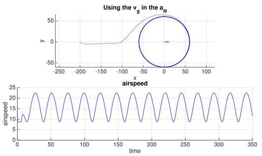
-250 -200 -150 -100 -50 0 50 100 x -50 0 50 y Using the v g in the aN 0 50 100 150 200 250 300 350 time 0 5 10 15 20 25 airspeed airspeed

Figure 2.3: Wind is 7 m/s, airspeeed starts at 14 m/s, and varies. The ground speed is used in the nonlinear acceleration command.

A way to still preserve a constant airspeed is to consider the vG in the nonlinear

acceleration command, but then only apply that component of the acceleration command which lies along the lateral body axis.

Even though this approach partially compensates for the wind, it entails a severe discrepancy for slow vehicles, resulting in non easily predictable behaviours which are largely undesirable and must be taken care of one by one: as an example, at a given moment we could have ˆvG ⇡ ˆL, that incorrectly results in aNM ⇡ 0. An

example of such suboptimal behaviours is shown in figure 2.4.

2.3.2

Proposed strategy

Here the goal is to find the control input uslow that satisfies the requirements in

2.8. We first find a basic control input, called ue, and improve on that to obtain

uslow. To this end, we are going to reason in steady state, i.e.

8 > < > : e = 0 ˆ TG = ˆTP d ˆTG dt = d ˆTP dt (2.18)

Initial control input

Here we are going to satisfy the first two requirements in (2.8). It is useful to consider the geometry of the problem shown in Figure 2.5 and introduce the following angles

15 2.3. The Lower Wind Case -50 0 50 100

east (meters)

north (meters)

Corner Case: turn around

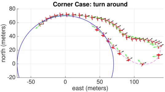
Figure 2.4: Initially, the ground speed is almost aligned with the look-ahead vector, hence the aircraft is not commanded to change its attitude and gets carried away by the wind. The aircraft is forced to perform a complete turn around to get back on track.

( e = arccos ˆw· ˆL0 y = arccos wˆ _{· ˆ}L1e = ⇡ e arcsin (w ?_{sin (} e) v? M ) (2.19) where ˆL1e is an unknown target orientation for the aircraft to be computed. It

should be noted that these angles are not defined in case w = 0. We now aim to satisfy the first two requirements stated in (2.8) through the choice of a basic control input

ue = kˆL1e (2.20)

To find such a command, we assumed to already be at the Position/Orientation steady state condition. Since we assume to be on the path with the desired orientation, then k(vM ⇥ ˆL1e)⇥ vM = 0, meaning that ˆTM = ˆL1e ( ˆTM = Lˆ1e

would be an unstable equilibrium, as showed in [1]).

The natural choice for the desired groundspeed direction is ˆL0, as it was defined

in 2.16. Note that ˆL0|e=0 = ˆTP. We need to find the desired direction ˆL1e for

the aircraft by solving the geometry shown in picture 2.5, which means solving the following equation in ˆL1e:

w + v? MLˆ1e

kw + v? MLˆ1ek

17 2.3. The Lower Wind Case The solution, in terms of the angles defined in (2.19), is

( ˆ L1e = sign([ ˆw⇥ ˆL0]· k)rot( ˆw, y) w? > 0 ˆ L1e = ˆL0 w? = 0 (2.22)

where rot(a, ✓) is the function that rotates vector a 2 R3 _{by angle ✓ around}

the vertical axis k. The basic ue will be improved in 2.3.2 to obtain curvature

convergence.

Improvement of the control input to satisfy the curvature convergence requirement

Again, we will reason in steady state. In order to satisfy the curvature conver-gence requirement, we need that

(aN_M · ˆNP)|rM=rP, ˆTG= ˆTP = kPkvGk

2 _(2.23)

So we define a (scalar) amount of additional normal acceleration to be applied for the vG to keep the curvature as

kaGN resk = kkvGk2k(ˆL0⇥ ˆL)⇥ ˆL0k (2.24)

ˆ

L and ˆL0 as defined in 2.2.3. It’s easy to verify that

kaG N resk |e=0 = kkvGk 2_k(ˆT P ⇥ ˆL|d|=dshift)⇥ ˆTPk =_kkPkkvGk2 (2.25)

The idea is to rotate the ue = kˆL1e by a proper angle ✓s, which is shaped soon

after. If we do so, then in steady state the normal acceleration applied to the vehicle will not be null but

kaMN resk = kv?M2sin (✓s) (2.26)

When w = 0 we have v?

M =kvGk, then we can trivially observe that kaG_{N res}k =

kaM

N resk. As kaGN resk is obtained through (2.24), then considering (2.26) we can

already obtain the needed shifting angle:

✓s = arcsin [sat(k(ˆL0⇥ ˆL)⇥ ˆL0k)] (2.27)

where ˆL defined as in 2.14, the sat(·) function bounds the argument to be in the interval [-1,1]. As to the general case w? _{> 0, where the angles}

e and y

where ⌦ is the angular speed vector V is the linear speed vector. Then, using the angles introduced before, it holds

8 > > > < > > > : ˙_{e =} kaGN resk kvGk ˙y = ˙e w?cos ( e) ˙e v? M q 1 (w?sin( e) v? M ) 2 (2.28)

Since it is also true that ˙y = ka

M N resk

v? M

, by comparison with the (2.26) we obtain the formulation for ✓s

✓s = arcsin [sat(

˙y kv?

M

)] (2.29)

The conclusion is that by choosing the control input

uslow = rot(ue, ✓s) (2.30)

ue defined as in 2.20, the goals in (2.8) are satisfied. We report in Figure 2.6 a

phase portrait showing global convergence in numerical simulations for a large variety of initial conditions and di↵erent windspeeds. That said, attractiveness to the equilibrium will have to be formally proved in future work. In Figure 2.7, we can observe the performance of the algorithm for strong constant wind, still slower than the airspeed.

Choice of k

Still we have to determine the parameter k. In order for the algorithm to keep null error in steady state, we have as a lower bound on the choice of k:

k > max_|kP|4w

?

v? M

|kP| (2.31)

The lower bound on k can be derived from the worst case scenario (ˆL0 = ˆw,

groundspeed in favour of the wind) by posing the argument of the arcsin in equation (2.29) to be in the interval [-1,1] when e = 0. If we pick an even greater k, it is also possible to guarantee that the argument of the arcsin will not ever saturate during the transient when e _{6= 0, resulting in better transient} performance.

2.4

The Higher Wind Case

Let us define the desired direction for the groundspeed ˆL0 as in equation (2.16),

and the corresponding basic control input ueas in equation (2.20). It is convenient

to reason considering the angles introduced in (2.19): refer to Figure 2.8 for a better visualization.

19 2.4. The Higher Wind Case -50 0 50 η [deg] -150 -100 -50 0 50 100 150 e* [m] -50 0 50 -150 -100 -50 0 50 100 150 -50 0 50 -150 -100 -50 0 50 100 150

Figure 2.6: Phase portraits of the proposed lower wind solution for w?_{=0 m/s}

(left), 7 m/s (middle), and 13.5 m/s (right), respectively. The tracking angular error ⌘ = atan2⇣TˆPy, ˆTPx

⌘

atan2⇣TˆGy, ˆTGx ⌘

2 [ ⇡, ⇡] is compared with the signed, one-dimensional cross-track error e⇤ _{= e·} rM

krMk to demonstrate algorithm convergence within the bounds of BL = 50 m, for k = 0.05, R = 100 m, and

v?

-200

-150

-100

-50

0

50

x

-60

-40

-20

0

20

40

60

y

Proposed Solution

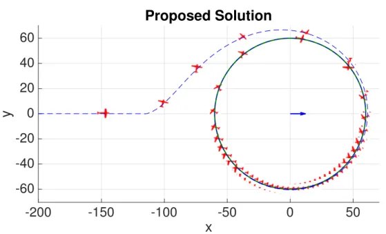
Figure 2.7: Airspeed 14 m/s. Windspeed 12 m/s. The proposed control input lets the vehicle achieve the objectives stated in 2.8.

y

Figure 2.8: Geometry: w? _{> v}? M

21 2.4. The Higher Wind Case

2.4.1

Solution for ˆ

L

feasible

As the desired groundspeed direction ˆL0 is feasible, the idea is then to reason

as in 2.3.2: choose the basic control input ue as in (2.20) and shift it by the

correct shifting angle ✓s in order to achieve curvature convergence: this would

mean ufast,1 = uslow, and doing so we would achieve curvature convergence as

long as the ˆL0 continues to be feasible. However, with usual shapes for the target

curved path, at some point the desired direction will become infeasible: when this happens, we need the control input not to change abruptly, i.e. to be a continuous function of the desired ˆL0. Since we cannot in general achieve the goals in (2.8),

we actually make a slightly di↵erent choice for ufast,1 that guarantees continuity

in the sense mentioned before (as better explained in [2]), while keeping almost perfect curvature convergence as long as the ˆL0 is feasible:

✓s2 = q [1 (w?sin ( e) v? M ) 2_] cos ( e) ✓s (2.32)

So, in the end,

ufast,1 = rot(ue, ✓s2) (2.33)

2.4.2

Infeasible desired direction: the state of the art.

As anticipated, the case of windspeeds being so strong as to force the aircraft to fly backwards is usually neglected in the field of aeronautics, as it is a pretty rare event. This is indeed quite frequent with LALE UAVs.

When this happens, the main goal we can easily think of, as the aircraft is bound to flow away from the target path together with the wind, is to “minimize the damage”: this results in trying to minimize the norm of the groundspeed. This is achieved if the aircraft turns against the windfield.

The easiest way to do so is to instantaneously ask the aircraft to turn against the wind as soon as it is not possible for it to follow the desired path, and hope for the wind to stop: this is what was done before starting this thesis.

Although this could be a suitable emergency way of acting in case the windspeed rarely overcomes the aircraft airspeed, this is indeed suboptimal and could result in very poor tracking performance in the case of persisting strong winds.

In Figure 2.9, an example of such suboptimal behaviour is shown:

As soon as the target direction becomes infeasible, the aircraft abruptly turns against the wind, and cannot change its mind until the direction becomes feasible again “by chance”. Another reason why this behaviour is undesirable can be seen by thinking of a wind profile that often crosses the line between w? _{< v}?

M and

w? _{> v}?

M: as the commands would be largely discontinuous, this would result in

-50 0 50 x -60 -40 -20 0 20 40 60 y

Stronger Winds, Old Approach

Figure 2.9: Wind is 15m/s, directed from left to right, airspeed is 14m/s.

2.4.3

Solution for ˆ

L

infeasible

We define an infeasibility parameter ↵out and a safety function safe(↵out) as

follows: ↵out = ⇡ safe = ⇡ 2 y(↵out) ⇡ 2 (2.34) both indices have maximum value equal to 1. When safe= 1, it means that we act

conservatively and choose ufast,2

k = w: this has to happen only in the absolutelyˆ

worst scenario of ˆL0 = w, which corresponds to the maximum ↵ˆ out = 1. In

all the intermediate cases, we want to guarantee a tradeo↵ between conservatism and tracking performance, i.e we want safe(↵out) to be increasing with ↵out.

This can be achieved by finding a proper mapping f from angle ⌫ = ⇡ e to

angle y in the following form

f : ⌫ 2 [0, ⇡ ]! y 2 [0,⇡

2 ] (2.35)

This mapping should satisfy the following 3 properties: f (0) = 0 f (⇡ ) = ⇡ 2 f (a) < f (b) _{8a > b, a, b 2 [0,}⇡ 2 ] (2.36)

The first requirement is to guarantee that safe = 1 when ˆL0 = w. The second

one is a boundary condition to guarantee that the input is continuous to the ˆL0

23 2.4. The Higher Wind Case is for finding a tradeo↵ between safety and performance: put in words, the more the ˆL0 is infeasible for the groundspeed, the more we want to turn against the

wind and wait for it to stop.

By looking at picture 2.8, a natural choice that follows geometric intuition and is coherent with the requirements that we have just stated, is

ufast,2 = k p w?2 _v? M2Lˆ0 w kpw?2 _v? M2Lˆ0 wk (2.37) In terms of the mapping that has been defined before, this choice corresponds to

f (⌫ = ⇡ ) = y = arcsinp sin ⌫ cos

1 + cos2 _{+ 2 cos cos ⌫} (2.38)

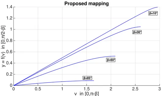
this mapping satisfies the requirements (2.36), as can easily be verified by sub-stitution and derivation with respect to ⌫. For clarity, the function is plotted in Figure 2.10 for di↵erent values of the wind-cone opening angle

0 0.5 1 1.5 2 2.5 3 0 0.2 0.4 0.6 0.8 1 1.2 1.4 Proposed mapping

Figure 2.10: proposed mapping y = f (⌫) for di↵erent values of In Figure 2.11 the performance of the algorithm is shown.

It is also worth highlighting the tradeo↵ introduced between performance and security (incremental safety) by computing the safety function safe(↵out) :

safe= ⇡

2 + arcsin (

sin (⇡ (⇡ )↵out) cos p

1+cos 2_{+2 cos cos (⇡ (⇡ )↵out)})

⇡ 2

(2.39) as is also shown in Figure 2.12.

-150 -100 -50 0 50 100 x -40 -20 0 20 40 60 80 y

Higher-Winds: proposed strategy

Figure 2.11: wind is 16 m/s, airspeed is 14 m/s. The proposed law is used. Magenta line: feasible desired direction. Red line: infeasible desired direction

0 0.2 0.4 0.6 0.8 1 out 0 0.1 0.2 0.3 0.4 0.5 0.6 0.7 0.8 0.9 1 safe Infeasibility/Safety tradeoff

25 2.5. Proof Of Stability

2.5

Proof Of Stability

We are in the scenario of w? _{> v}?

M. For finite-length paths, we want to show that

we achieve the requirements in 2.9.

Here we will also consider briefly the case of infinite paths: the only realistic case in UAV application is that of infinite linear paths. In this case we want to show

that: ₈ < : lim t!1a M N(t) = 0 ˆ TM t!1= rot( ˆw, f ( ⇡ 2 µ)) (2.40) where µ = arccos ˆw· ˆ⇤, ˆ⇤ is the direction of the target linear path, mapping f : ⌫ _{! y has to be chosen. The second requirement in 2.40 asks for a tradeo↵} between the linear-path direction and the anti-wind direction for the ˆTM, that

results in an efficient direction for the actual ˆTG.

In both cases, the proof for the proposed algorithm will be structured as follows: • First the so called geometric case will be tackled: the vehicle is considered

to always be at the desired heading angle, i.e. ˆTM(t) = ufast,2_k (t), 8t.

• Then, the so called dynamical case (the vehicle is not always at the desired heading angle) will be considered and shown to fall into the geometrical case as time goes to infinity.

2.5.1

Geometric case: finite paths

Subcase 0. Single point path

Here we consider the path to be very far away and hence similar to a single point P for the aircraft to be reached. The radially shifted distance is indistinguishable from the error, so ✓s(t) ⇡ 0 8t. Also, notice that with a point-path, ˆe = ˆL0. By

defining a = q w?2 _v? M2, l =kaˆL0 wk (2.41) we obtain vG⇥ ˆL0 = (w?+ vM? Lˆ1e)⇥ ˆL0 = = (w + v ? M(ˆL0a w) l )⇥ ˆL0 = = ((1 v ? M l ) | {z } >0 w + av ? M l Lˆ0)⇥ ˆL0 = (1 v ? M l ) | {z } >0 w_{⇥ ˆ}L0+ 0 (2.42)

Now let the line directed as ˆL0 divide the plane into two half-planes: the previous

considerations imply that vGand w both lie in the same half-plane, so the ˆL0will

rotate more towards the w direction in time until eventually lim

t!1

ˆ

L0 = lim t!1ˆe =

ˆ

w. Another way to see this: the path-point P acts as a rotational joint for the error vector e, which is fixed at one end in P : the vG is rotating the error

vector in the same direction as the wind would rotate it, meaning that it will point instantaneously more in the anti-wind direction, i.e. even more outwardly with respect to the cone, until it reaches the anti-wind direction (the “torque” around point P is null at that point).

As in this case ˆL0 = ˆe, the ˆL0 rotation must stop here. Since f (0) = 0, then also

lim

t!1 ufast,2

k = w by construction. By hypothesis of geometrical case, this meansˆ

lim

t!1

ˆ

TM(t) = w. Then, by definition of the normal acceleration command, alsoˆ

lim

t!1a M

N = 0 so we reach asymptotic safety as defined in 2.9.

As an additional feature, note that

sign[(vG⇥ w) · k](t0) =

sign[(vG⇥ w) · k](t), 8t > t0 (2.43)

so we reach the equilibrium without oscillations around that line such that ˆe = ˆ

w.

Subcase 1. Finite length paths

In this case, the ˆL0 versor is a function of the particular path we are considering,

so we can no longer assume it to coincide with ˆe as in the single point path case. However, consider the following two facts:

• The path is finite

• 8t 2 R, rM(t)· ˆw rM(0)· ˆw + (w_| ?_{zvM? _}) >0

t

That is, as the wind is constantly stronger than the airspeed, the minimum growth of the projection of the error onto the wind direction has rate (w? _v?

M)t. This

implies that

lim

t!+1krM(t)k = +1 (2.44)

and since the path is finite lim

t!+1kd(t)k = limt!+1ke(t)k = +1 (2.45)

As the distance grows to infinity, the path will look like a single point P1, that

is the center of the smallest circle that contains the whole path. Then, we fall into the single point-path subcase.

27 2.5. Proof Of Stability

2.5.2

Geometric case: infinite linear paths

Here the path is not finite. However, a common case in UAV applications is when the path is an infinite line. If this line is outside the wind-cone or the intersection with the cone is finite, it is not possible for the vG to align to it. In this case,

the proposed algorithm achieves efficient wind stability, i.e. the objectives in 2.40. To show this, simply notice that if d > BL, then whatever the vehicle

position, we have ˆL0 ? ˆ⇤, as the error direction will always be perpendicular to

the line. A simulation for this situation is shown in Figure 2.13.

The interpretation for this result is that the proposed algorithm finds some effi-cient compromise for the vG direction between the anti-wind direction and the

path direction, which is a tradeo↵ between safety and tracking performance.

0 100 200 300 400 500 600 x (meters) 200 250 300 350 400 450 500 y (meters)

Efficient Wind Stability

Figure 2.13: Airspeed is 14 m/s. Windspeed is 30 m/s, indicated by the magenta arrow on the aircraft. ˆ⇤ = (p₂2,p₂2). Line direction is hence infeasible.

2.5.3

Dynamical case

Here we will extend the proof for the geometric case, so as to consider the dy-namics imposed by the nonlinear acceleration command. As the subcase of finite-length paths was shown to fall into the subcase of single-point paths, studying the dynamic extension for the single-point paths is all we need. The extension for the infinite linear path is trivial and will be omitted, as the ˆL0 stops changing

as soon as d > BL.

In the following, it is clearer to directly refer to Figure (2.14) for the symbols definition.

y z

path

E E

Figure 2.14: Symbols used in the proof Subcase 1

If

< ⌫ < ⇡ (2.46)

corresponding to ˆL0 pointing outside of the “specular” cone, then it is easy to

see that

↵Lg < ⇡, 8✓g (2.47)

meaning that

˙⌫ < 0 (2.48)

independently from the actual aircraft orientation. This holds until we fall into subcase 2.

Subcase 2 If

29 2.5. Proof Of Stability corresponding to ˆL0 pointing inside of the “specular” cone, we need further

con-siderations. It is not true anymore that ↵Lg < ⇡, 8✓g. Instead we have

(

↵Lg < ⇡, if ✓g > ⌫

↵Lg ⇡ otherwise

(2.50) Then it’s possible that, depending on how the aircraft is oriented, ⌫ will increase while the angle between ˆTM and the commanded direction ufast,2_k is smaller than

⇡, which is undesirable as it would mean the ˆL0 is “running away” from ˆTM.

To show that eventually the aircraft can be considered to be aligned with its commanded control input versor ufast,2

k , consider the following:

• We can increase parameter k in order to make the vehicle turn with faster dynamics.

• As time goes to infinity, eventually the “chasing” angle z will decrease to 0.

To show this last fact, first notice that for any given ˆTM, if ˙⌫ > 0 then ˙⌫ is a

decreasing function of|e · w| that goes to 0 as 1

|e·w| or faster. Indeed, consider the

case when ˙⌫ > 0 and has the maximum value, i.e. ⌫ = 0 and ˆTM?w. We have

˙⌫MAX=

v? M

|e · w| (2.51)

which acts as an upperbound for all the other situations. Irrespectively from ˆTM,

since w? _{> v}?

M, |e · w| indeed increases, hence ˙⌫ must decrease and tend to 0.

Since y is a function of ⌫ such that_{8 ⌫, y(⌫) < ⌫, than also ˙y decreases and tends} to 0 as time goes to infinity. Now consider the time derivative of the “chasing” angle z

˙z = ˙y + ˙⇠ (2.52)

Since we showed lim

t!+1˙⌫(t) = 0 = limt!+1˙y(⌫(t)), irrespectively of what the

orien-tation of the vehicle could be at any time, then, as ⇠ indicates the heading angle of the aircraft,

lim

t!1˙z(t) = ˙⇠(t) (2.53)

As the acceleration command is designed to steer the vehicle orientation onto the chosen look-ahead vector, which now is ufast,2

k , as the look-ahead is bound to

asymptotically stop changing as the vehicle gets further away from the path, then we actually have that lim

t!1˙⇠(t) = 0, with the vehicle aligned to the look-ahead

vector. This, together with the 2.53, translates in lim

t!1z(t) = 0 (2.54)

Then we can say that we asymptotically fall into the geometrical case, and the proof holds.

2.6

Continuity

In realistic scenarios, the wind is not going to be constant, but will likely switch between w? _{< v}?

M and w? > vM? several times. Not only that, the path is going

to be curved, so the desired direction for the groundspeed ˆL0 is going to switch

between being feasible and infeasible. All these switchings mean that it is very important for the command input u to be continuous to changing winds and changing ˆL0.

The control input was derived separately for the three subcases (slower winds, higher winds with feasible desired direction, higher winds with infeasible desired direction) in 2.3, 2.4.1, 2.4.3. We want to show here that the complete control input u = 8 > < > : uslow, w?  v?M ufast,1, w? > v?M,  ufast,2, w? > v?M, > (2.55) indeed guarantees continuity in this sense.

• Switching between uslow and ufast,1: this happens as the wind passes

from w? _{< v}?

M to w? > vM? . Let t⇤ be the boundary time instant in which

w?_(t⇤_{) = v}?

M(t⇤). Also, in this case, e(t⇤) ⇡₂. Looking at the formulation

for ✓s and ✓s2 in (2.32), we have:

✓s2|w?_=v?

M = ✓s|w?=v?M (2.56) and so uslow(t⇤) = ufast,1(t⇤)

so the command u(t) is continuous at this boundary condition

• Switching between uslow and ufast,2: this happens as the wind passes

from w? _{< v}?

M to w? > vM? . Let t⇤ be the boundary time instant in which

w?_(t⇤_{) = v}?

M(t⇤). Also, in this case, e(t⇤) > ⇡₂. Solving the geometry in

2.5, we have that ue = w. Since (t⇤) = ⇡₂, this implies that y(t⇤) = 0

as computed in (2.38): so ufast,2(t⇤) = w as well. Assuming ˆTM ⇡ ˆL1e,

which is the case after some transient, we have thatkvGk ⇡ 0. So by (2.28),

we have ✓s⇡ 0, implying

uslow(t⇤)⇡ w ⇡ ufast,2(t⇤) (2.57)

• Switching between ufast,1 and ufast,2: this happens when w? > vM and

ˆ

L0 passes from being feasible to being infeasible. Let t⇤ be the boundary

time instant. Then

31 2.6. Continuity so ✓s2(t⇤) = 0. This guarantees continuity, as no shifting angle is applied in

the infeasible case.

In Figure 2.15 we report a plot that highlights the continuity of the input as the wind increases and for a fixed ˆL0. We indicate the associated angles y for the u

direction and ⌫ for the ˆL0.

0 5 10 15 20 25 30 35 40 windspeed (m/s) -0.5 0 0.5 1 1.5 2 2.5 3 3.5 y (rad) Mapping between L 0 and L1e

Figure 2.15: Switching w? _{lower/higher than v}?

M. Magenta: inside the cone.

2.6.1

Sinusoidal Winds

As an example of a more realistic varying wind profile, in order to show that the commands do not switch abruptly and are continuous, we consider the case of the wind having this sinusoidal profile

w(t) = W sin (⌦t)⇥1 0 0⇤T (2.59)

for some wind pulsation ⌦ and amplitude W > v?

M. The result is shown in Figure

2.16, and the same is shown (more clearly) in an accompanying video1_.

Switching between any couple of the three parts of the control input can happen in this case. The least smooth behaviour, as we have only approximate continuity, is when the switching is between uslow and ufast,2.

2.6.2

Rotating Winds

The wind has the following expression

w(t) = W ⇥cos ⌦t sin ⌦t 0⇤T (2.60)

-80 -60 -40 -20 0 20 40 60 x -60 -40 -20 0 20 40 60 y

Sinusoidal High Winds

Figure 2.16: Sinusoidal winds. Blue: uslow is applied. Magenta: ufast,1 is applied.

33 2.6. Continuity for some wind pulsation ⌦ and amplitude W > v?

M. When the direction becomes

feasible, the vehicle exploits the wind so as to progress faster on the path while keeping the curvature. During the unfeasible direction parts, it tries to follow the progression of the circle. This also helps in making the required direction feasible again in a shorter time, as the wind rotates. This would be impossible with the old methods. A plot can be seen in Figure 2.17. An accompanying video is provided2_.

-80

-60

-40

-20

0

20

40

60

x

-60

-40

-20

0

20

40

60

y

Rotating High Winds

Figure 2.17: Rotating high winds. Magenta: faster wind, inside wind-cone. Red: faster wind, outside wind-cone

2.7

Roll Dynamics

The guidance algorithm was developed by considering the vehicle to behave as a point-mass, i.e. we assumed that each acceleration command from the nonlinear guidance could be matched perfectly and instantaneously by the vehicle. This is clearly not the case for a nonholonomic vehicle such as the fixed-wing UAV. In particular the nonlinear lateral dynamics of a fixed-wing UAV can be described in north-east coordinates as follows ([20]):

8 > > > > > > < > > > > > > : ˙n = v? Mcos + wn ˙e = v? M sin + we ˙ = g tan_v? M ˙ = p ˙p = b0 cmd a1p a0 (2.61) where we wn T

= w is the nonlinear wind e↵ect, g _{⇡ 9.81 is the acceleration} of gravity, is the heading of the aircraft (computed from the north-axis), is the roll angle that translates into if we enforce the so called coordinated turn hypothesis that holds in steady-state flight ([21]), and the parameters a0, a1, b0

describe the roll-dynamics, i.e. the dynamics between a roll command and the actual aircraft roll.

From the equations, we can deduce the transfer function between roll commands and actual roll:

(s) cmd(s) = b0 s2_{+ a} 1s + a0 (2.62) Higher order dynamics could be used, however it has been found in [20] through the identification procedures, that second-order fits appropriately the closed loop low-level autopilot attitude control response. The test-bed platform available in ASL-ETHZ is shown in Figure 2.18

Through the identification procedure outlined in [20], it was possible to identify the roll dynamics for the Techpod:

b0 = 13.48 a1 = 6.577 a0 = 13.97 (2.63)

In order to translate the acceleration aN

M into a roll command cmd, a simplified

formulation was derived from the coordinated turn hypothesis ([21]):

cmd = arctan (k a M Nk

g ) (2.64)

where g is the acceleration of gravity and is a parameter we can choose to achieve better performance. Usually = 1 is a proper choice.

35 2.8. Flight Results

Figure 2.18: Fixed-Wing Test Platform: Techpod. Credits to [20]

With the real data at hand, some simulations were run to observe the perfor-mance of the nonlinear algorithm on the Techpod.

In figure 2.19, the wind is such that w? _{< v}?

M, so we showed in 2.3.2 that the

proposed guidance algorithm let the point-mass vehicle achieve the goals in 2.8, i.e. position/orientation/curvature convergence. As the algorithm does NOT consider the actual roll-dynamics directly, however, it is not possible to achieve perfect convergence. A delicate tuning of the parameters k and BL, can partially

take care of the roll-dynamics and make it possible to achieve very good perfor-mance. A simulation with the Techpod roll-dynamics and strong wind still such that w? _{< v}?

M is shown in Figure 2.19.

As to the case of w? _{> v}?

M, the same considerations hold. Thanks to a fine tuning

of the parameters it was possible to achieve good tracking performance and the objectives in 2.9. A simulation is shown in Figure 2.20.

2.8

Flight Results

The proposed algorithm was implemented on a Pixhawk Autopilot in C++, and thoroughly tested in HIL simulations. This was necessary to obtain a fine-tuning of the control parameters in the guidance law and be sure everything was right before actually flying. Subsequently, it was tested on a small fixed-wing UAV in high wind conditions. The Pixhawk Autopilot platform is shown in Figure 2.21. The test-bed platform aircraft for these flight tests was the so called “EasyGlider” (Figure 2.22, whose identification step gave the following minimum order roll-dynamics:

(s)

cmd

= 1.649

-150 -100 -50 0 50 x -80 -60 -40 -20 0 20 40 60 80 y Techpod Roll-Dynamics

Figure 2.19: Wind is 10 m/s, flowing from left to right. Airspeed is 14 m/s. Techpod Roll Dynamics are considered.

After successful implementation, in Figure 2.23, 2.24, we show the results (taken directly from the stored data in the IMU of the aircraft) from the flight tests. The aircraft was commanded to follow a circular trajectory in counter-clockwise direction at a nominal airspeed of 8 m/s. The wind vector is represented in the figures using the following arrow, color scheme: w? _{< v}?

M (black), w? >

v?

M \ (ˆL0 feasible) (magenta), w? > vM? \ (ˆL0 infeasible) (red).

In Figure 2.23, the UAV can be seen to attempt curvature following despite the infeasible look-ahead direction until a point where the wind speed reduces and allows the start to convergence back to the path.

Figure 2.24 shows a wind-stabilized approach towards the trajectory until the point where simply pointing into the wind is the only option to reduce “runaway” from the track, recall the tracking direction is counter-clockwise.

37 2.8. Flight Results -200 -100 0 100 200 x -200 -150 -100 -50 0 50 100 150 y

High Wind: Techpod

Figure 2.20: Wind is 15 m/s, flowing from left to right. Airspeed is 14 m/s. Techpod Roll Dynamics are considered.

Figure 2.21: The PixHawk PX4 plat-form. Credits to [3]

Figure 2.22: The EasyGlider PRO. Credits to http://www.green-eyes.it/Modellismo/EasyGlider.htm

0 20 40 60 80 100 east (meters) -60 -40 -20 0 20 40 60 north (meters) Flight Test

Figure 2.23: First moment from the flight test

-100 -50 0 50 east (meters) 0 20 40 60 80 100 120 140 160 north (meters)

Real Flight Test

Chapter 3

A Guidance Approach Based On

Model Predictive Control

In this chapter, we will investigate a completely di↵erent guidance approach. In chapter 2, we developed a novel nonlinear guidance algorithm able to cope with arbitrarily strong windfields: the solution is easy to implement and computation-ally very light, however the following should be noted.

• Having in mind the application to real fixed-wing UAVs, we cannot assume that the acceleration commands from the nonlinear guidance law will be matched perfectly by the (nonholonomic) vehicle. This will result in the necessity of fine-tuning the control parameters very carefully for each dif-ferent aircraft and for each path, depending on the wind profile, which is doable but inconvenient in many situations.

• The tradeo↵ between performance and safety does not consider the mini-mization of a cost function, and relies on the particular choice we make for the mapping function 2.35. This means the tradeo↵ is built upon common-sense, and cannot be the mathematically best choice in every situation. We are giving up on optimality in exchange for simplicity and computational lightness.

For these reasons, it seemed natural to compare the performance of the proposed nonlinear algorithm with a controller based on an optimizer. As the model of the aircraft we can obtain is not perfect and the wind profile can vary in time, we chose to implement a Model Predictive Controller (MPC).

The MPC control framework is briefly outlined in 3.1. The application to fixed-wing UAVs is described in 3.2. After shofixed-wing some preliminary simulation results in 3.3, the reshaping of the cost function to envision the possibility of winds such that w? _{> v}

M? and obtain the safety objectives in 2.9 is described in 3.4. Finally,

simulation results are shown in 3.5.

3.1

The (Nonlinear) MPC Framework

The introduction about MPC given in this section is partially quoted from the Preface of the book [22], as it is a very clear introduction to the problem.

Dynamic optimization has become a standard tool for decision making in a wide range of areas. The basis for these dynamic optimization problems is a dynamic model in the form

˙x(t) = f (x(t), u(t)), x(0) = x0 (3.1)

that describes the evolution of state x(t) in time as it is influenced by a control input u(t). In general, function g(_{·) is a nonlinear function of its arguments. The} goal of the dynamic optimization is to find, at each time ⌧ , that control input u([⌧, ⌧ + N ])? _{(where [⌧, ⌧ + N ] indicates the time interval between ⌧ and ⌧ + N )}

such that some objective function is optimized over some time horizon [⌧, ⌧ + N ], for some chosen N .

Usually, the minimization of the objective function takes the following form: min

u(⌧,⌧ +N )

Z ⌧ +N ⌧

q(x(t), u(t))dt + p(x(⌧ + N )) (3.2) The terms q(x, u) and and p(x) are referred to as the stage cost and terminal cost. Many realistic problems can be put into this framework and a lot of algo-rithms and software packages are available to come up with the optimal input u([⌧, ⌧ + N ])?_{. Even large problems described by complex models and involving}

many degrees of freedom can be solved efficiently and reliably.

To this point, it seems that finding the proper u([⌧, ⌧ + N ])? _{is everything we}

need: however, this structure still lacks some feedback to compensate for model imprecision and external disturbances, which combined could make the system deviate from its predicted future behaviour. This would ruin the procedure and make it unreliable.

For this reason, it is common practice to measure the state after some time pe-riod, say one time step, and to solve the dynamic optimization problem again, starting from the measured state x(⌧ +Tst) (where Ts is the time needed for two

consecutive sensing steps) as the new initial condition. This feedback of the mea-surement information to the optimization endows the whole procedure with a robustness typical of closed-loop systems.

A big limitation of MPC is that running the optimization procedure online at each time step requires a huge amount of time and computational resources. However, as explained in [22], “today, fast computational platforms together with advances in the field of operation research and optimal control have enlarged in a very significant way the scope of applicability of MPC to fast-sampled applications. One approach is to use tailored optimization routines which exploit both the

41 3.2. The MPC Guidance Approach For Fixed-wing Vehicles structure of the MPC problem and the architecture of the embedded computing platform to implement MPC in the order of milliseconds.

The second approach is to have the result of the optimization pre-computed and stored for each state in the form of a look-up table or as an algebraic function u(t) = g(x(t)) which can be easily evaluated. Whatever approach we may choose, the optimization guidance is not easy to implement and generally require a great amount of on-board computational power.”

3.2

The MPC Guidance Approach For

Fixed-wing Vehicles

Several control schemes based on Model Predictive Control were developed in the literature. In [23], a nonlinear model predictive controller (NMPC) is built on the kinematic fixed-wing model of the UAV, in order to track a desired line, and a stability analysis is performed. In [24], this approach is extended to tackle the case of multiple line segments with obstacle avoidance. In [25], the problems inherent to real-time implementation are tackled: an adaptive-horizon approach is proposed based on the curvature of the target path. An alternative approach based on model predictive control and backstepping techniques is proposed in [26].

The case of windy scenarios is directly tackled in [27], but the wind is supposed to be slower than the aircraft airspeed. We are indeed interested in tackling the case of arbitrary windspeeds.

To test the algorithm which will be proposed in the following, we took the frame-work described in [20]. There, the formulation and implementation of a Nonlin-ear MPC controller for general high-level fixed-wing lateral-directional trajectory tracking was developed. The ACADO Toolkit [28] for generation of a fast C code based nonlinear solver was used.

The optimization problem takes the following form min

u,x

Z T t=0

⇣

(y(t) yref(t))T Qy(y(t) yref(t)) + (u(t) uref(t))T Ru(u(t) uref(t))

⌘ dt + (y(T ) yref(T ))T P (y(T ) yref(T ))

subject to ˙x = f (x, u) y = h(x, u) u(t)_{2 U} x(0) = x(t0)

where h(x, u) is the selection function that maps states and inputs into the pe-nalization variables that appear into the objective function. The choice of the proper penalization variables for the application at hand is very important, as we will see in what follows. Considering the aircraft dynamics in 2.61, we come up with the state vector x = ⇥n e p⇤T and the control input u = cmd. As

the set of achievable rolls is bound, then U denotes the (convex) set of possible inputs, which is directly taken into account into the optimization problem. The standard approach is to create the following error variables

et= e· ˆNP

e = d

(3.4)

where e, ˆNP are the same as defined in 2.2, d = arctan 2

⇣ ˆ

TPe, ˆTPn ⌘

, =

arctan 2(vGe, vGn). So, et represents the track-error and e represents the course error, i.e. how much the groundspeed direction is di↵erent from the tangent di-rection to the path at its closest point.

Having defined these error variables, the usual choice for the penalization vari-ables vector is the following:

y =⇥et e p r

⇤T

(3.5) By a proper choice of the weight matrices Qy, Ru, P it is then possible to achieve

convergence to arbitrarily shaped paths, provided the maximum curvature does not exceeds the minimum turn-radius of the aircraft at its maximum speed (which is when the wind is in favour of the aircraft).

However, the ratio of the weights inside matrix Qy is tricky to be chosen, and

depends on both the path shape and the wind profile.

Taking inspiration from the Look-Ahead method in [1], in order to have a simpler tuning, we created the following penalization variable:

eLˆ = arctan 2 ⇣ ˆ Le, ˆLn ⌘ (3.6) where ˆL is chosen as in 2.13, and considered the following penalization variables vector:

y =⇥e_Lˆ p r

⇤T

(3.7) By doing so, we are actually dividing the tuning step in two parts:

• Tune the parameters k, BL for the Look-Ahead guidance, in order to define

the desired behaviour we want to see the aircraft perform.

• Tune matrices Qy, Ru, P , but this is much easier than before as we don’t