Topographic and geomorphologic modeling and analysis of the
bedrock surface beneath Ultimi Lobe ice-cap (South Pole,
Mars) using MARSIS high-resolution data.
Relatore: Presentata da:
Prof. Andrea Morelli Giacomo Di Silvestro
Correlatori:
Prof. Roberto Orosei Dott. Luca Guallini
Sessione III
ABSTRACT
Lo scopo del presente lavoro è stato quello di definire la topografia e le principali morfologie del basamento roccioso al di sotto di una porzione, Ultimi Lobe (UL), della calotta polare meridionale di Marte. Tramite l'analisi dei radargrammi MARSIS per mezzo di una procedura di mappatura semi-automatica sviluppata in MATLAB, è stato possibile ricavare i dati altimetrici della superficie subglaciale in questione. Successivamente, attraverso il metodo di interpolazione noto come Natural Neighbor (Sibson, 1981), è stato possibile creare in ambiente software ESRI ArcGIS un modello di elevazione digitale della superficie.
Quest’ultima ha permesso un’analisi innovativa delle geomorfologie presenti sul basamento della calotta polare al fine di comprenderne i processi geologici di formazione, l’eventuale correlazione tra ciò che viene osservato in superficie e quanto già scoperto alla base della calotta polare (vedi regione dei laghi; Orosei et al., 2018) e, infine, i possibili eventi che hanno caratterizzato la suddetta porzione del ghiacciaio in periodi remoti. In particolare, i risultati ottenuti hanno contribuito: 1) A fornire nuove prove sull’origine tettonica di alcune morfologie superficiali note come Large Asymmetric Polar Scarps (LAPS; Grima et al., 2011); 2) A descrivere ed analizzare possibili morfologie glaciali; 3) Ad individuare in corrispondenza del lago subglaciale individuato da Orosei et al. (2018) una serie di alti e bassi topografici funzionali al contenimento d’acqua.
Tutti questi elementi suggeriscono un lento scorrimento di parte della calotta glaciale di UL in tempi remoti, forse favorito da un flusso di acqua di fusione alla sua base come la rete di laghi subglaciali scoperta da Orosei et al. (2018) e Lauro et al. (2021) sembrerebbe suggerire. Questi ultimi, infatti, potrebbero essere ciò che rimane di più ampi deflussi passati.
SUMMARY
1 INTRODUCTION ... 1
2 MARS PHYSICAL PROPERTIES ... 4
2.1 GEOPHYSISCAL MEASUREMENTS AND ORBITAL PARAMETERS ... 4
2.2 MARS POLAR ICE CAPS ... 9
2.2.1 NORTHERN POLAR ICE-CAP: PLANUM BOREUM ... 11
2.2.2 SOUTHERN POLAR ICE CAP: PLANUM AUSTRALE ... 14
3 OBSERVATIONS AND MARS MISSIONS ... 20
3.1 MARS MISSIONS ... 21
3.1.1 Mars Global Surveyor ... 21
3.1.2 Mars Odyssey ... 21
3.1.3 Mars Express ... 22
3.1.4 Mars Reconnaissance ... 23
3.1.5 ExoMars ... 23
3.2 INSTRUMENTS AND TECHNIQUES ... 25
3.2.1 MARSIS ... 25
3.2.2 MOLA ... 26
3.2.3 REMOTE SENSING AND SAR ... 27
3.2.4 RADAR ECHO SOUNDING ... 32
4 DATA ANALYSIS ... 40
4.1 RADARGRAMS ... 40
4.2 DATA PROCESSING CODE PROGRAMMING ... 42
4.3 THREE-DIMENSIONAL SURFACE MODEL ... 45
4.3.1 INTERPOLATION TECHNIQUES ... 45
5 GEOMORPHOLOGIC AND TOPOGRAPHIC ANALYSIS OF THE BEDROCK SURFACE... 51
5.1 OVERALL MORPHOMETRIC AND TOPOGRAPHIC DESCRIPTION ... 52
5.2 NEW EVIDENCE ABOUT LAPS FORMATION ... 54
5.3 ANALYSIS OF POSSIBLE GLACIAL MORPHOLOGIES ... 59
5.4 SOME CONSIDERATIONS ABOUT THE “SUB-GLACIAL LAKE DISTRICT” BEDROCK TOPOGRAPHY ... 67
6 CONCLUSIONS AND FUTURE PROSPECTS ... 70
BIBLIOGRAPHY ... 72
1
1 INTRODUCTION
Human curiosity has always brought people to look at the night sky and wonder what there could be above our heads and what is our place in this vast sea of emptiness that we called the Universe. This search for an understanding has accompanied Humankind since the dawn of civilization all around the globe. The first moon landing was not only a technological success but also a giant evolutionary leap that humanity achieved as a species. Preparing the ground for the next space exploration is the first task to complete to see Humankind leaving its cradle and cooperating under the same flag. Mars is our closest neighbor with similar properties to the Earth, being not only a suitable candidate for a hypothetical colony but a window for a better understanding of our planet and the solar system. Its current state may shed light on eventual future problems that could strike Earth, whether for natural or anthropic reasons. Therefore, understanding its evolution is critical either for both to predict a possible change in climatic and geological conditions that may occur on Earth, and thus prevent problems related to it, and to better understand geological and physical mechanisms that we are not yet able to explain or fully understand. The technological discoveries that research in the space field has brought have found application in the most diverse fields, offering a significant contribution even in those disciplines distantly related to it. The benefits that space exploration has brought, and those that it promises to bring, have led several nations to invest in it. The number of missions launched towards the Red Planet in the last decades has reached remarkable dimensions, seeing the entry into the game also of China, India, and Arabs Emirates. The economic potential present in space research has also led private companies to join the table of contributors, becoming the visionary protagonists of what could be the same story that more than 500 years ago has radically changed the geopolitical situation of the Earth. It is not clear what could be the new Palos of the XXI century, and little we care, but the premises that bring with them a possible (but I dare to define, even for idealistic spirit, certain) success of Mars colonization plans are revolutionary. The changes that this event promises to bring about are not only economic, social, and technological, but also philosophical and
existential. Recent discoveries made below the Martian south polar cap, which will be mentioned several times later in this paper, are nothing short of amazing. The presence of a network of
subglacial lakes (Orosei et al. 2018 and Lauro et al. 2021) in a hostile environment, characterized by extreme physical conditions, ignites a glimmer of hope regarding the possibility of finally answering one of the most complex questions that have accompanied humankind for millennia: are we the only
2
sailors adrift in interstellar space aboard a gravitational prison, or is our existence not something so unique and rare? It is clear that if it is shown that not only the conditions that have allowed the existence of these bodies of water also support the existence of complex molecules, but that these conditions are even found in multiple places on the planet, the discovery of extraterrestrial life forms would not be so unlikely. On the tail of these recent discoveries, the main aim of the present work is to provide a better understanding of the topographic, morphological, and geological context of the buried region located under the south polar ice-cap and encompassing the water reservoirs defined by Orosei et al. (2018) and Lauro et al. (2021) based on radar permittivity. In particular, using selected orbits collected by the MARSIS radar instrument aboard the European probe Mars Express, net of the limitations imposed by the instrument, by the data density, and by the processing algorithms, we defined a three-dimensional model of the bedrock underlying a portion of the ice-sheet known as Ultimi Lobe. This model facilitates the identification of peculiar geomorphologies, allowing us to give a plausible interpretation of the possible causes and events that led to the formation of these structures and, thus, to give a valid interpretation, under a strict geological point of view, on the origin of the subglacial lakes of Orosei et al. (2018). To achieve this purpose, several processing and interpretational steps have been necessary, starting from the writing of a code in MATLAB for the analysis and recovery of data from radargrams collected by MARSIS. Through that, we calculated the elevation of the basal surface of the cap in the points where the probe has made sampling. We then proceeded with the interpolation of the data to create a georeferenced map aimed at studying the topographic and morphological properties that characterize the buried bedrock surface. This allowed us to identify geological structures probably related to past glacial movements and basal melting, and also to define a series of basins and depressions consistent with the accumulation of subglacial lakes (in contrast with the conclusions of previous authors, i.e., Arnold et al., 2019 and Sori and Branson, 2019, suggesting local thermal anomalies). Among those, the study also helped to understand the origin of some structures in UL known as LAPS and studied by Grima et al (2011).
Schematically, the present manuscript has been organized:
• Describing the geological context of Mars and the Martian poles, along with the description of the physical properties of the planet and the most important missions and instruments by NASA and ESA.
3
• Describing the geodetic techniques and instruments used in the space missions that enabled the collection of the data used in the present work.
• Describing and analyzing the used software and algorithms, the data, and the methodologies used.
• Analyzing and interpreting the topography, geomorphology, and geology of the modeled bedrock surface in comparison with what is observed at the surface and on Earth in similar environments.
4
2 MARS
PHYSICAL
PROPERTIES
2.1 GEOPHYSISCAL
MEASUREMENTS
AND
ORBITAL
PARAMETERS
The orbit of a body around a center of mass is described in geodesy by six Keplerian parameters, three accounting for the orientation of the orbit and three for its dimension and shape (the sixth parameter is the current position of the object in the orbit in a specific instant of time expressed as the fraction of the orbital period) [Tab. 1].
Mars is the fourth planet from the sun with a distance of 2.2792×10⁸ km (semimajor axis). The shape of the orbit, as suggested by the eccentricity ‘e’, is not perfectly a circle but rather an ellipse,
characterized by a minor and a minor axis orthogonal to each other. Tab. 1 Orbital properties of Mars
Semimajor axis 2.2792×10⁸ km
Eccentricity 0.0933941
Inclination 1.84969142
Longitude of ascending node 49.55953891°
Longitude of perihelion Sideral orbital period Synodic orbital period Mean orbital velocity Maximum orbital velocity Minimum orbital velocity Obliquity Perihelion Aphelion 336.0563704° 686.98 days 779.94 days 24.13 km s-1 26.50 km s-1 21.97 km s-1 25.19° 2.066×10⁸ km 2.492×10⁸ km
Source: JPL Solar System Dynamics page: ssd.jpl.nasa.gov/ and NSSDC Mars Fact Sheet: nssdc.gsfc.nasa.gov/planetary/factsheet/marsfact.html
5 ⅇ =√𝑎 2− 𝑏2 𝑎 (1) ⅇ′=√𝑎 2− 𝑏2 𝑏 (2) 𝑓 =𝑎 − 𝑏 𝑎 (3)
with 𝑎=semimajor axis and 𝑏=semiminor axis, f=flattening
A Martian year corresponds to 686.98 Earth days and a sidereal day is 24h 37m 22.65s, slightly longer than the terrestrial period of 23h 56m 4.09s. Due to the oblateness of the orbits and the
obliquity of the rotational axis, the Mars surface is subject to change in the degree insolation. For the vernal equinox, first day of spring in the northern hemisphere, the longitude of the Sun (Ls) as seen from Mars is Ls=0°. Northern hemisphere summer solstice occurs at Ls=90°, northern autumnal equinox is at Ls=180°, and northern winter solstice occurs at Ls=270° (Carr, 1981). The southern hemisphere experiences warmer summer than the northern cause the perihelion (position of
maximum proximity to the Sun) occurs near Ls=250° near the summer solstice and as a consequence,
Figure 1 Keplerian parameters
source: https://it.mathworks.com/matlabcentral/fileexchange/72098-keplerian-orbit
6
a colder winter. During the cold seasons, Mars atmosphere start to condensate on the poles, forming the seasonal caps thanks to the precipitation of CO2 ice with smaller amounts of H2O ice and dust. Activity begins around Ls=185° for the northern hemisphere, during the autumnal equinox, and near Ls=50° for the southern hemisphere, mid-autumn (Dollfus et al., 1996), and becomes visible near Ls=10° in the north and Ls=180° in the south. Image 3 and 2 shows thickness and precipitation variations.
The influence of the solar system celestial bodies, and its two moons Phobos and Deimos, causes perturbation of the Martian orbit resulting in variations in Mars Orbital parameters [a precession with a rate of -7576 milli-arcseconds yr-1 (Folkner et al.1997).]. These variations are mostly periodical and alter the amount of radiation that reaches the surface at different latitudes, in the case of obliquity and eccentricity variations. Due to the spin-orbit resonance, Mars rotational axis inclination
undergoes a short-term variation with a ~120 kyr period (Ward, 1973). Also, the eccentricity varies with periods of about 95 to 99 kyr and 2400 kyr of a value between 0 and 0.12 (Laskar et al., 2001; 2004). The argument of perihelion varies with a period of 51kyr and the orbital inclination varies between 0 and 8° occurring every 1.2 Ma (Fishbaugh et al., 2008). Obliquity varies from 0 to 80° with a most probable value of 41.8° (Laskar et al., 2004) and with a 63% probability of it being >60° in the past billion years (Fishbaugh et al., 2008). The Martian obliquity exerts the greatest influence, oscillating about its present mean value (25°) with a period of 1.2x10⁵ y and with an amplitude of oscillating that varies with a period of 1.3x10⁶ y (Ward, 1992; Laskar & Robutel, 1993; Touma and Wisdom, 1993; Laskar et al., 2004). The main influence on the ice caps bulk, as has been previously Figure 3 Elevation residuals referenced to 50N & S. The figure, obtained from the MOLA
data, shows ~160 profiles in each hemisphere of the mean residual in each 1-degree latitude band.
Source: Smith & Zuber, 2018
Figure 2 Maximum accumulation of CO2 vs
latitude. The average increase in depth is ~5 cm/degree. The maximum depth in the northern hemisphere occurs at the edge of the permanent cap. In the southern hemisphere the precipitation appears to increase almost linearly with altitude. Source: Smith & Zuber, 2018
7
said, is the distribution of solar radiation on the surface which dictates the annual rate of accumulation and sublimation of H2O and CO2 ice.
Tab. 2 Physical properties of Mars
Mass 6.4185×10²³ kg
Volume 1.6318×10¹¹ km3
Mean density 3933 kg m-3
Mean radius 3389.508 km
Mean equatorial radius North polar radius South polar radius Sidereal rotation period Solar day Flattening Precession rate Surface gravity Escape velocity Bond albedo
Visual geometric albedo Blackbody temperature 3396.200 km 3376.189 km 3382.580 km 24.622958 h 24.659722 h 0.00648 -7576 milli-arcseconds yr-1 3.71 m s-2 5.03 km s-1 0.250 0.150 210.1 K Source: Data from Smith et al. (2001) and NDSSDC Mars.
Fact Sheet: nssdc.gsfc.nasa.gov/planetary/factsheet/marsfact.html
Another parameter to consider is the percentage of dust in the atmosphere, that absorbs the solar radiation coming directly from the Sun and reflected by the surface. Dust deposition also lower the ice-surface albedo, increasing the amount of radiation absorbed at the surface. The albedo is predominantly controlled by the amount of CO2 deposited during the fall and winter seasons and
carbon dioxide ice clouds may affect infrared emission. The PLD (polar layered deposits, see section 2.2.1.3 & 2.2.2.3) may undergo variations due to impacts of meteorites and volcanic eruptions which melts the ice and alter the amount of dust diluted in the atmosphere. However, volcanic influences
8
during the Deposits lifetime are extremely rare and so not responsible for the bulk impurities of ice. There are many ways in which the obliquity may affect the climate, but the effects are not easily predictable. For example, the climate warming might lead to an increase in surface pressure, increasing the dust deposit and lowering the albedo, hence leading to cooling. At the same time, a decreasing climate temperature may lead to an increased ice stability and consequently a higher albedo. At very low obliquity 10°-15°, the atmosphere collapses and condenses onto the surface, with distribution controlled by topography (Kreslavsky and Head, 2005). At present-day low
obliquity, ground ice is stable only at latitudes above 60°-70° (Mellon and Jakosky, 1995). There is a global distribution of ground ice a few meters above the regolith when the obliquity reaches 32° and the temperature at the equator gets lower (Mellon and Jakosky, 1995).
But at the same time, the climate at the poles gets warmer and the ice is unstable (Mischna et al.,
2003). Glacial features at mid-latitudes, such as lobate debris aprons and lineated valley fills, may testify for these assumptions. The Hesperian-aged south circumpolar Dorsa Argentea formation has Figure 4 The diagrams represent the quasi-periodic variation of the insolation with respect to Mars orbital eccentricity and axial obliquity astronomic cycles during the last million year (left) and ten million years (right). Credits: Images adapted from Grima (2009) (top-left) and Laskar et al. (2002) © Nature (bottom)
9
been interpreted to be an ancient polar deposit underlying the present SPLD and extending over twice the area of the current PLD (Head & Pratt 2001).
2.2 MARS
POLAR
ICE
CAPS
Before going deep with the data analysis, we will discuss the main properties of the north and south ice caps. The general structure of both polar caps consists of an upper seasonal CO2 dome (Forget
1998), a permanent water-ice cap (Kiefferet al.,1976; Kiefferet al.,1979; Paige et. al 1990 polar ice caps), and a Polar Layered Deposits unit (PLD) lying above the Martian bedrock (Fig. 5).
As previously said, to obtain information regarding the thickness and composition of the caps we need to understand the dielectric properties of the materials that are distributed within and
underneath the polar caps. The bedrock composition varies depending on the geological history of the planet and the degree of porosity which cause a mixture of rocks and liquid or glacial intrusion by the overlain Polar Layered Deposits. As suggested by the NASA Pathfinder APXS and the chemical classification of lava (Picardi et al., 2005), the dielectric constants, within which the
Figure 5 Polar caps structure schematic representation. Vertical scale exaggerated by a factor 150 for the layered deposit, by an unknown factor for the permanent cap and a factor 50000 for the seasonal cap. Source: Greve 2008
10
Martian surface materials may vary, are proper of Basalt and Andesite, two igneous rocks of low and intermediate silica content respectively (Tab. 3).
Tab. 3 Dielectric properties of the subsurface materiel Source: Picardi et al., 2005
Basalt Andesite
𝜺𝒓 7.1 3.5
tanδ 0.014 0.005
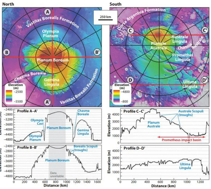
Figure 6 Regional MOLA topographic maps showing the north (left) and south (right) polar regions at the same scale. Red lines indicate locations of topographic profiles. Gray shading in north polar profiles indicates the region for which topographic data are unreliable. Parallels are plotted every 5◦. 0◦E is at the bottom in the north polar view and at the top in the south polar view. Source: Byrne, 2009
11
2.2.1 NORTHERN POLAR ICE-CAP: PLANUM BOREUM
2.2.1.1 NORTHERN SEASONAL ICE-CAP
Many of the characteristics of the northern Northern Ice Cap (NIC) are in common with those
described in the southern one. Structures and composition are almost the same with some distinctions mostly due to the different degrees of insolation caused by the orbit eccentricity around the Sun. The northern pole, in fact, is characterized by warmer winters, resulting in an overall seasonal ice cap thinner than the southern one (it is generally 1.5-2 m thick) that sublimates completely during the summer (Mesick & Feldman 2020). Another difference is that while the southern Seasonal Ice Cap (SIC) rises above the surrounding terrain, the northern one, extending to 60°N symmetrically to the pole, lies near the bottom of the North Polar basin (Zuber et al., 1998; Head et al., 1999).
2.2.1.2 NORTHERN RESIDUAL ICE-CAP
With a volume of 1.1-2.3x10^6 and a diameter of 1100km (Zuber et al., 1998; Smith et al., 2001), the northern Residual Ice Cap (RIC) mostly covers Planum Boreum reaching a height of 3 km (the highest region of the north cap approximates the position of the present rotational pole; Fishbaugh & Head, 2001). On the contrary to the southern pole, the northern RIC does not contain CO2 layers but
Figure 7 Northern ice cap picture from Mars Orbiter Camera of the MGS orbiter
Source:
https://www.nasa.gov/mission_page s/MRO/multimedia/pia13163.html
12
only water ice. Moreover, the albedo of the surface (Bass et al., 2000; James and Cantor, 2001; Kieffer and Titus, 2001; Malin and Edgett, 2001; Hale et al., 2005) suggests the presence of dust impurities in the icy layers and changes of grain size (Warren and Wiscombe, 1980; Kieffer, 1990; Langevin et al., 2005). OMEGA instrument, which provides the mineralogical and molecular
composition of the surface of Mars through imagery and infrared spectrometry, indicates a maximum dust content of about 6% (Langevin et al., 2005). The northern RIC surface is characterized by different morphological features, resulting from the ablation of the ice and erosion by strong wind and forming pits, cracks, and knobs. Also, the RIC displays a series of spiral troughs that reach the underneath North PLD (i.e., depths up to 1km) with a clockwise pattern (Zuber et al.,1998).
2.2.1.3 NORTH POLAR LAYERED DEPOSITS (NPLD)
Similar to the South PLD, the NPLD are composed of different strata of ice up to ten meters of thickness (Brothers et al., 2015) accumulated throughout its depositional history with various ice-dust fractions (e.g., Cutts & Lewis, 1982; Hvidberg et al., 2012). In particular, it is generally
Figure 8 North polar layered deposit computed thickness Source: Greve, 2008
13
accepted that 95% of the composition of the layers, showing a regional dielectric constant value of 3.15, consists of water ice (Grima et al., 2009; Picardi et al., 2005). The NPLD has a volume of 1.2±0.2×10⁶ km3 (polar ice caps) and their bulk density is 1,126 ± 38 kg/m3 (Ojha et al., 2019). The center of the NPLD unit is offset toward a 0°W longitude due to the retreat of the cap predominantly from the 180°W direction. At the same time, the highest elevation of the cap approximates the position of the present rotational pole (Fishbaugh & Head 2001). Like in the southern hemisphere, the NPLD are cut by a reentrant valley (i.e., Chasma Boreale), supposed to be originated by katabatic wind erosion (Kolb e Tanak, 2001) or catastrophic floods (Anguita et al., 2000), and a series of spiral troughs (far more numerous than in the south).
Figure 9 a, Individual and connected pits in surface of residual cap. Portion of Mars Orbiter Camera (MOC) image M00-00547 (mapping phase 0, image 547), 82.1° N, 329.6° W, solar incidence angle i = 73°. Texture on most of the north-polar residual cap is a variant of pitting of approximately similar width depressions; length and connectivity of depressions varies. Depths inferred from minimal evidence of shadows are probably less than 2 m. Scale bar is 200 m. Illumination is from upper right. Aerocentric longitude of the sun (Ls) is 120° (0° is northern spring equinox). 5 April 1999. This and other images shown have been contrast enhanced. b,
North-polar residual cap surface, portion of image CAL-00433; 86.9° N, 207.5° W; scale bar is 50 m. Illumination is from upper right. Ls =
107°. 8 March 1999. c, merging of pits and fissures of residual cap topography with exposure of layers in walls of one of the dark lanes (troughs with wall slopes generally less than 10°) that traverse much of the northern layered deposits; area at bottom of image is largely frost-free. Portion of MOC image M00-02072; 85.9° N, 258.1° W; i = 70°. Scale bar is 100 m. Illumination is from upper right. Ls = 124°. 13 April 1999. Source: Thomas et al., 2000
14
2.2.2 SOUTHERN POLAR ICE CAP: PLANUM AUSTRALE
2.2.2.1 SOUTHERN SEASONAL ICE-CAP
The Seasonal Ice Cap (SIC) is centered around the geographic pole (Barlow, 2014) and extends to a latitude of 50°S during the winter (Hansen et al., 2010). In the southern hemisphere, the SIC is characterized by thin layering -ten centimeters to meters- of CO2 ice (showing high reflectivity) that
sublimates during the summer and deposits during the winter. This mechanism is part of a seasonal cycle as a result of the planet's axial inclination and during which the carbon dioxide sublimates from one pole to move to the opposite one. This periodic process involves almost 25% of the atmospheric CO2 (Mesick & Feldman, 2020). The sublimation is helped in the southern hemisphere because it is
affected by higher temperatures than in the northern. In fact, at the south pole, the summer season occurs when the planet reaches the perihelion (Greve, 2018).
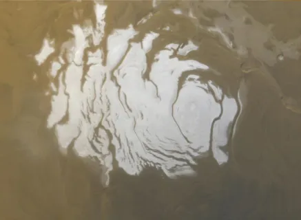
Figure 10 South polar cap picture from Mars Orbiter Camera of the MGS orbiter
Source:
https://www.nasa.gov/centers/ames/multimedia/imag es/2005/marscap.html
15 2.2.2.2 SOUTHERN RESIDUAL ICE-CAP
Figure 11 12 a, Nearly circular depression and nearby sag surface on top layer. Polygonal cracks are prominent on undisturbed sections of the upper layer surface, but do not affect the margins of circular depressions. Portion of MOC image M09-00609; 87.0° S, 5.9° W; i = 70°. Scale bar is 100 m. Illumination is from lower right. Ls = 237°. 3 November 1999. b, ‘Fingerprint’ pattern of
depressions. Elongated sags in other areas of residual cap suggest precursors of this topography. Steeper sides (right) of the troughs face in a more northerly direction, suggesting sublimation in expanding depressions, as with the more circular ones. Portion of MOC image M03-06756; 86.0° S, 53.9° W; i = 88°. Illumination is from lower right. Scale bar is 500 m. Ls = 182°. 4 August 1999. c, Circular
collapse features, leaving mesas on upper surface with debris aprons and moats. Largest scarps here are about 4 m high. The uppermost layer is capable of supporting scarp slopes of ∼20°; the aprons frequently have slopes of order 1°–3° (Fig. 2b); slopes are estimated from presence or absence of shadows as the sun gained elevation in the southern spring. Portion of MOC image M03-06646; 85.6° S, 74.4° W; i = 88°. Scale bar is 500 m. Illumination is from lower right. Ls = 181°. 3 August 1999. d, Residual mesa
exposing four layers and surrounding moat. Formation of moats probably requires additional deposition and sublimation or compaction following removal of material from height of top layer exposed here. Portion of MOC image M07-02129; 86.9° S, 78.5° W; i = 81°. Scale bar is 100 m. Illumination is from bottom, right. Ls = 204°. 11 September 1999. e, Complex covering of
depressions which suggest burial and exhumation of topography on part of the southern residual cap area. Portion of MOC image M04-03877; 84.6° S, 45.1° W, i = 81°, scale bar is 200 m. Illumination is from lower right. Ls = 196°. 29 August 1999.
16
The southern Residual Ice-cap (RIC) is characterized by an elevation 6 km higher than the northern one and is offset with respect to the planet rotational axis toward the 180°W longitude (Fishbaugh & Head, 2001). The RIC estimated volume is about 1.2-2.7x10⁶ km3 (Smith et al., 2001) and it has a diameter of about 400 km (Barlow, 2014). Data collected from Viking (Mouginot et al., 2008) and Mars Express orbiter indicate that the RIC is composed of a permanent upper CO2 ice-cap
overlapping water-ice layers. The residual cap is characterized by a thickness of 8 meters (Stevens, K. W. 2007) and by a dielectric constant of 2.2 (Mouginot et al., 2009). The sublimation and collapse of carbon dioxide veneer (Byrne & Ingersoll, 2003) produce a variety of morphologies, such as depressions with a wide variety of shapes (Thomas et al., 2000b).
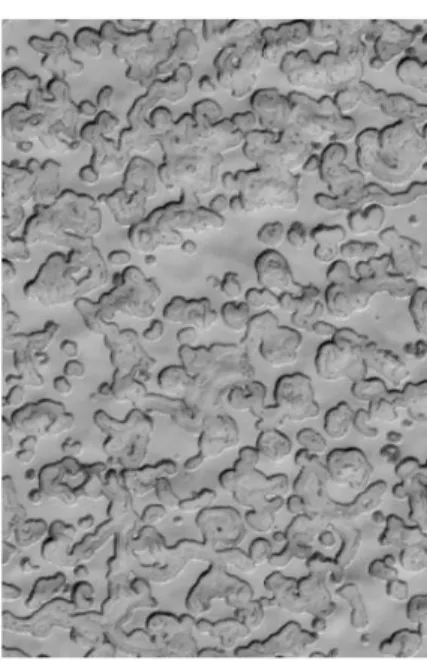
Figure 13 swiss-cheese’ terrain caused by the sublimation of CO2 ice on the
southern ice cap. (MOC image MOC2-780, NASA/JPL/MSSS)
17
2.2.2.3 SOUTH POLAR LAYERED DEPOSITS (SPLD)
The South Polar Layer Deposits (SPLD) underlies the RIC and represents the oldest unit of the southern polar-cap. SPLD are characterized by stratified layers of water ice and, in low percentage (5-10%; Heggy, 2006) of dust mixture silicate. Besides, composition models have shown dielectric constant consistent with the local interbedding presence of CO2 ice (Liu et. al, 2014). Also, the
SHARAD instrument has displayed CO2 deposits below Australe Mensa, having a volume of about 16,500 km3 (Putzig 2018). The deposits are offset from the pole by ~2° and are asymmetrically distributed between latitudes 70° and 80°S. It has been estimated (Herkenhoff & Plaut, 2000) that the surface age of the South Polar Layered Deposits (about 10 Ma) is two orders of magnitude greater
than the surface age of the NPLD (at most 100 ka). The centers of symmetry of the northern and southern planform shapes are asymmetrical about the current rotational pole; therefore, they are offset few degrees from the pole in antipodal directions from each other (Tanaka and Scott 1987, Smith et al., 1999, Fishbaugh and Head 2000a, Ivanov and Muhleman 2000). The ice-dome shows spiral scarps that have a counter-clockwise pattern extending from the pole, dissecting the residual cap, outward into the PLD to 82.5°S; this feature could be caused (both in the southern and northern)
Figure 14 South polar layered deposit computed thickness Source: Greve, 2008
18
by the preferential sublimation of ice from the sun-facing slopes (Howard et al., 1982), enhanced by strong katabatic winds produced by the sublimation and deflected by the Coriolis force (Howard, 2000). As an alternative, it could be modeled by non-homogenous ice-flows from the accumulation center of the ice-cap toward the ablating edges (Fisher 1993; Fisher 2000). A large reentrant valley, Chasma Australe, cut the deposit for several hundred kilometers with a width of about 20 km (Anguita et al., 2000). The volume of SPLD has been evaluated around 1.6±0.2×10⁶ km3 (Plaut et al., 2007), while the unit reaches a maximum thickness of 3.7±0.4 km in correspondence of the highest MOLA elevation, close to 0°E (Plaut et al., 2007). Among the large variety of
geomorphological structures and findings on Planum Australe, two of them represent the departure point of the object of the present study: 1) A series of scarps with a unique shape. Grima et al. (2010) analyzed and described some morphologies, distributed all over the SPLD, but condensed in Ultimi Lobe. These features appear to be arch-shaped with a cross-section characterized by a trough
between a straight slope on one side with outcrops of layered deposits and a convex upward slope on the other one that flattens as it rises. These semicircular structures, defined as Large Asymmetric Polar Scarps (LAPSs) can reach a length in the order of tens of kilometers. Furthermore, some of them are aligned and/or appear connected with a relatively uniform direction (Fig. 15), where the concave sides never face the South Pole, and the dominant orientation is not toward the azimuth. The extremely deep troughs formed by LAPSs in the ice create scarps whose height ranges from 200 to 700 m with an average of 400 m, penetrating the glaciers to part of its thickness. The side of the
scarps with a convex slope shows a more complex topography. The ascending wall gently curves Figure 15 (Top) Histogram of the LAPS azimuths. The Y-axis is the number of occurrences. A concavity facing north has an azimuth equal to 0. A concavity parallel to a longitude and facing decreasing west-longitudes has an azimuth equals 90. (Bottom) Circular histogram of the relative orientation of the LAPSs in a regional context. The circle border represents 25 occurrences. Source: Grima et al., 2011
19
until it flattens out. Along certain scarp crests ridge similar to elongated hillocks may overly these formations.
2) Recent studies made by Orosei et al. (2018) based on the high value of the medium permittivity have shown the presence of liquid water beneath the SPLD in a 20 km wide zone centered at 193°E, 81°S, then confirmed by further geological and physical studies of a wider zone (Lauro et al., 2021).
Figure 16 Shaded topography of UL (stereographic projection with illumination from the bottom-right). The white line is the Planum Australe boundary. The bottom-right insert locates UL within the entire polar plateau. Black boxes (A, B, C, D, E) outlining the LAPSs. Source: Grima et al., 2011
20
3 OBSERVATIONS
AND
MARS
MISSIONS
First observations with a telescope, were made by Galileo in 1609 followed by many others such as Huygens with the first report of albedo marking, Cassini who noticed for the first time the bright polar caps, and Herschel in 1783 when he determined the inclination of Mars' rotation axis. Mars has been a major spacecraft destination ever since the early days of space exploration mostly cause one of the biggest questions was concerning the possibility to find alien life on other planets besides Earth. Until these days many nations have been involved in the production and expedition of Orbiters
Figure 17 All Spacecraft Missions to Mars since 1960. Planetary society https://www.planetary.org/space-images/the-mars-exploration-family-portrait
21
and Landers toward the Martian body (Fig. 17), the more important missions regarding the recent observation of the Polar Caps are Mars Global Surveyor, Mars Odyssey, Mars Express, Mars Reconnaissance Orbiter, and ExoMars.
3.1 MARS
MISSIONS
3.1.1 Mars Global Surveyor
The Mars Global Surveyor spacecraft reached mars’ orbit in 1997 with an average altitude of about 378 km. The observations made, have provided information regarding the state of the magnetic field (which has ceased to exist -except some remnant magnetization within the rocks- caused by the recent absence of an internal dynamo), the thickness variation of the crust on both hemispheres, the shape of the gravitational potential, general surface and polar caps composition based on the albedo, erosional effects of wind and water fluxes on the ground and atmospheric circulation. The
instruments that made possible these evaluations were: Mars Orbiter camera, an imaging system designed to take high spatial resolution images of the surface and lower spatial resolution, synoptic coverage of the surface and atmosphere, Mars Orbiter Laser Altimeter, a laser pulse altimeter able to determine globally the topography of Mars by generating high-resolution topographic profiles, Thermal Emission Spectrometer to study trough the thermal infrared emission of the planet the surface and the atmosphere of Mars and a Magnetometer/Electron Reflectometer suitable for the study of any magnetic fields (Albee et al., 2001).
3.1.2 Mars Odyssey
The Mars Odyssey spacecraft reached the Martian orbit in 2002 with an orbit of 370 to 432 km above the ground and in an inclination of 93.1°. The goal was to map the elemental composition of the surface, determine the abundance of hydrogen in the shallow subsurface, acquire high spatial and spectral resolution images of the surface mineralogy, provide information on the morphology of the surface, and characterize the Martian near-space radiation environment as related to radiation-induced risk to human explorers. The instruments onboard were: Thermal emission Imaging System to determine the mineralogy using multispectral, thermal- infrared images, Gamma Ray
22
gamma-ray and neutron spectroscopy, and the Martian Radiation Environment Experiment to measure the exposure of tissues to radiation (Saunders et al., 2004)
3.1.3 Mars Express
The ESA Mars Express mission was launched in June 2003 from the Baikonur Cosmodrome in Kazakhstan over a Soyuz rocket and reached Martian orbit in December of the same year. The mission carried an orbiter and a lander, Beagle 2, which never sent any signal back from the surface of the planet, to study together with the inventory of water or ice in the Martian crust and to gather evidence about any form of life, if ever there was one. Beagle 2 was supposed to land on Isidis Planitia, an impact basin characterized by layered deposits of sedimentary rocks probably generated by the water and surrounded by a variety of igneous rocks and craters of different ages, to study the geology of the ground together with the mineralogical and chemical composition. The spacecraft carrying the lander separated from the orbiter during the collision course, crossing the atmosphere in 5 minutes, five days after the split. The actual condition of Beagle2 is still unknown. The orbiter was placed in an elliptical near-polar orbit of 86.5° inclination and a period of about 7.5h with an
apocenter of 11500 km and a pericenter of 250km(sci.esa.int). The spacecraft consists of various instruments for the breakdown of the surface and subsurface properties and the analysis of the atmosphere. There are 6 instruments, in addition to a radio-science experiment, which deals with the solid (HRSC; OMEGA; MARSIS) and those analyzing the atmosphere (PFS; SPICAM; ASPERA). The MaRS radio science experiment provides insights into the internal gravity anomalies, the surface hardness, the neutral atmosphere, and the ionosphere of Mars. The PFS is an IR spectrometer for atmospheric studies. The main goal is to observe the variations of the global temperature in the long-term along with the chemical composition of the aerosol. SPICAM is a UV and IR spectrometer which studies photochemistry and the density-temperature structure of the atmosphere (0 - 150km), the upper atmosphere-ionosphere escape process, and the effect of the solar wind. The ASPERA experiment focuses on the upper part of the atmosphere affected by the solar wind; moreover, it analyzes the interaction with the near-Mars plasma and neutral gas environment. HRSC instrument consists of a very high-resolution camera that captures all the geomorphological features to
comprehend the influence of the water and weathering on the surface. The near-IR spectrometer OMEGA uses the signals in the infrared spectrum to differentiate the mineralogy of the surface and analyze the distribution of CO2, CO, H2O, dust, aerosol in the atmosphere. Mars Advanced Radar
23
for Subsurface and Ionosphere Sounding (MARSIS) is a low-frequency nadir-looking radar sounder and altimeter with ground-penetration capabilities operated. It uses synthetic aperture techniques (Chicarro et al., 2004).
3.1.4 Mars Reconnaissance
The Mars Reconnaissance Orbiter spacecraft entered Mars’ orbit in 2006 with a low near-polar orbit of 255 to 320 km. The main objective was to gain information concerning the geology, geophysics, climate, and volatile characteristics of the planet, find a clue about the possible presence of life forms and assess the nature and inventory of resources on Mars in preparation for human exploration. The observations were conducted with the help of different instruments such as the Mars Color Imager consisting of two framing cameras for the investigation of the weather conditions and the ozone for the evaluation of water vapor content in the atmosphere. The Mars Climate Sounder, a remote sensing device that works in the spectrum of the thermal infrared, provides a vertical profile for water vapor, dust, and temperature. Compact Reconnaissance Imaging Spectrometer for Mars uses detectors that see in visible, infrared, and near-infrared wavelengths to search for the residue of minerals that form in the presence of water, perhaps in association with ancient hot springs, thermal vents, lakes, or ponds that may have existed on the surface. The High-Resolution Imaging Science Experiment and the Context Imager can take pictures from orbit respectively at high and moderate resolution. The Shallow Radar works this the same principle of the MARSIS instrument with the focus on Martian regolith (Zurek et al., 2007). The data collected from the Mars Advanced Radar for Subsurface and Ionosphere Sounding of the ESA's mission Mars Express and the Mars Orbiter Laser Altimeter on the Mars Global Surveyor spacecraft have been used in this work.
3.1.5 ExoMars
The ExoMars program, which has seen an enormous contribution from Italy, is split into two parts. The first one concerns the launch, which happened in 2016, of an orbiter -the Trace Gas Orbiter (TGO)- around Mars and a lander -Schiaparelli- which never reached the surface. The second part consists of a rover and a surface platform which will be sent to the Red Planet in 2022. TGO is concerned with the detection of trace gases, gases that are present in small concentrations in the atmosphere, and their spatial and temporal evolution. What we are trying to do with this probe is to
24
define in a detailed way the atmosphere of Mars, observe the characteristics of the Martian soil to identify the sources of these gases, and map the subsurface hydrogen.
The tools it carries are: Nadir and Occultation for MArs Discovery (NOMAD) which features three spectrometers for identifying atmospheric components. Atmospheric Chemistry Suite (ACS) three infrared instruments that will support NOMAD. Color and Stereo Surface Imaging System (CaSSIS), a high-resolution camera to determine the geologic context of gas sources. Fine Resolution
Epithermal Neutron Detector (FREND), which can detect hydrogen up to one meter deep and detect water ice in the subsurface.
The Schiaparelli lander consists of a platform (DREAMS) for sensing wind speed and direction, humidity, pressure, near-surface atmospheric temperature, atmospheric transparency (Solar Irradiance Sensor, SIS), and atmospheric electrification (Atmospheric Radiation and Electricity Sensor; MicroARES). The COMARS+ instrument would be responsible for detecting temperature and heat flux during the descent phase. The descent camera (DECA) on Schiaparelli had the task of imaging the landing site as it approaches the surface, as well as providing a measure of the
atmosphere’s transparency. INRI consists of a series of retroreflectors that turn towards the zenith, useful for localization of the module by other spacecrafts. The Exomars rover will perform
electromagnetic and neutronic surveys of the subsurface to understand the geological context of the landing site. The ultimate goal would be to identify traces of life forms, present or past. The rover will bring with it different instruments to solve these questions.
• The Panoramic Camera (PanCam) for the digital mapping of the terrain.
• Infrared Spectrometer for ExoMars (ISEM) for mineralogical analysis of the soil.
• Close - UP Imager (CLUPI) for capturing high-resolution images of Martian rocks, outcrops, and cores.
• Water Ice and Subsurface Deposit Observation on Mars (WISDOM) and Adron for characterization of subsurface stratigraphy and detection of subsurface water. • Mars Multispectral Imager for Subsurface Studies (Ma_MISS) will contribute to the
mineralogical and petrographic identification of recovered samples. • MicrOmega infrared spectrometer for mineralogical study.
• Raman Spectrometer (RLS) that will perform a task similar to MicrOmega with the addition of the identification of organic traces.
25
• Mars Organic Molecule Analyzer (MOMA) that will search for biomarkers.
The platform will remain stationary and study the surface at the landing site. It will capture images of the landing ground, monitor the atmosphere and climate, study the distribution of water in the subsurface, measure the exchange of volatiles between the surface and atmosphere, perform geophysical surveys, and monitor the radiation environment (sources:
https://www.cosmos.esa.int/web/exomars/instruments; https://www.asi.it/esplorazione/sistema-solare/exomars ).
3.2 INSTRUMENTS
AND
TECHNIQUES
3.2.1 MARSIS
The radar can work at altitudes lower than 900 km at frequencies that ranges from 1.3 to 5.5 MHz for subsurface sounding, with a bandwidth of 1Mhz, and 0.1 to 5.5 MHz for ionospheric sounding. These features allow us to map the distribution of liquid or solid water in the upper part of the crust and to put constraints on the electron content during a sol (Martian solar day) of the ionosphere which influences the measurements. The subsurface sounder has two channels comprised in the Radio Frequency Subsystem: the first is connected to a dipole antenna and contains both a receiver and a transmitter meanwhile the second has only a monopole antenna that can receive the signals off-nadir. The antenna subsystem hence consists of a monopole and a dipole antenna respectively 7 and 40, restricted to 20 for dynamical purposes, meters long. The MARSIS antenna, and consequently the very large footprint (~3 to 5 km), does not provide high spatial resolution, severely limiting the ability to define those micro- and meso-scale structures otherwise observable with higher resolution Radars, such as SHARAD (Orosei et al., 2018). The Transmitter controls the signal flow between the antenna and the receive electronics. The Digital Electronics Subsystem (DES) resides in the same box as the radio frequency electronics receiver, it selects the frequencies to be used during the
sounding and includes a reference oscillator, timing, and control unit, and the processing unit (Jordan et al., 2009).
26 3.2.2 MOLA
The main objective of the Mars Orbital Laser Altimeter is to obtain a topographic map of the whole planet thanks to his spacecraft quasi-polar orbit. This instrument uses a technique similar to the RADAR inspections for altimetry, called LIDAR, and has provided a high-resolution measurement of the topography of Mars. Specifically, MOLA uses infrared pulses at a rate of 10Hz and has a spatial resolution of ~1° with an absolute accuracy of 13 m with respect to Mars' center of mass (https://tharsis.gsfc.nasa.gov/MOLA/mola.php,Smith et al., 1999). The laser beam has a footprint on the surface of ~160 m and shot-to-shot spacing of ~330m. The Orbiter sends pulses to the ground and receives the returned signal reflected from the Planet's surface. The altitude (observable) is calculated from the travel time and the known speed of light through a simple
formula:
𝑎 = 𝑐𝛥𝑡
2 (4)
With the altitude, the speed of light, and the travel time. The satellite height over the reference geoid is subtracted from the values measured from the instrument, representing the elevations in terms of topography and eliminating the contribution due to rotation. The gravitational field model used for the geoid is the MGM890i, derived from MGS orbit calibration and tracking and older mission data (Smith et al., 1999). If additional corrections are at first neglected, we find the basic simplified altimeter equation:
ℎ = 𝑁 + 𝐻 + 𝑎 (5)
Figure 18 Basic concept of satellite altimetry. Source: Seeber, Satellite Geodesy
27
With the computed height above the ellipsoid, the surface topography above the geoid, and the distance between geoid and ellipsoid. (Fig. 18). The accuracy of the measurement includes contributions from radial orbit error. Instrument error, and geoid error.
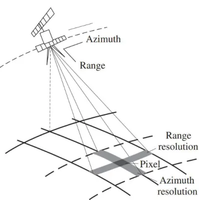
3.2.3 REMOTE SENSING AND SAR
A remote sensing image is characterized by pixels with a horizontal and a vertical resolution. Giving a beamwidth of 𝛥𝜃 (radians), with the antenna pointing perpendicularly to the ground, the azimuth resolution is simply:
𝛥𝑥 = ℎ 𝛥𝜃 (6)
Where:
𝛥𝜃 =𝜆
𝐿 (7)
𝜆 is the signal wavelength and 𝐿 is the aperture of the antenna. For what concerns the vertical resolution, considering a dipole antenna without an angular aperture of the beam in the range direction, we have to consider the rise time, that is the time that takes for the detected signal to go from zero to the maximum power.
𝛥𝑧 =𝑐 𝑡𝑟
2 𝑆 (8)
With S the signal-to-noise ratio
Another important thing is the frequency at which the pulses are emitted. If the frequency is high enough and the platform speed is low, the footprints (area on the surface illuminated by the beam) will overlap. Since each one of these samples is independent, and there are ( 𝑓 ℎ 𝛥𝜃
𝑣 ) of them, the vertical resolution when these samples are averaged becomes:
28
𝛥𝑧 = 𝑐 𝑡𝑟 2𝑆 √
𝑣
𝑓 ℎ 𝛥𝜃 (9)
This operation can improve the resolution, but if the Pulse Repetition Frequency (PRF) is too high, it would be difficult for the system to distinguish each pulse. So, the PRF must be lower than 𝑐
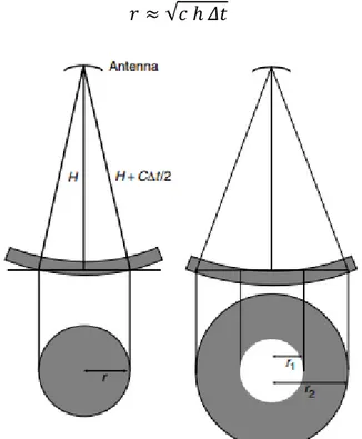
2ℎ to avoid the signals flying simultaneously. We will try to better understand the concept of 'rise time'. Assuming an ideal flat plane without scatterers, the received power will simply be proportional to the area illuminated by the beam. The transmitting pulse duration is tp and can be visualized as a
'scattering zone' of thickness 𝑐 𝑡𝑝
2 propagating away from the antenna. The first signal will be received at 2ℎ
𝐶. At a time 𝛥𝑡 greater than this one but smaller than 𝑡𝑝, the wave intersects the surface in a disk of radius r, see figure19. This disk expands over time until 𝑡 =2ℎ
𝑐 + 𝑡𝑝 when the trailing edge of the scattering zone just touches the surface. At 𝑡 =2ℎ
𝑐 + 𝛥𝑡, where 𝛥𝑡 is greater than 𝑡𝑝, the scattering zone intersects the surface in an annulus with inner radius 𝑟1 and outer radius 𝑟2, as shown at the right of figure 19. In the first case
𝑟 ≈ √𝑐 ℎ 𝛥𝑡 (10)
Figure 19 Simplified geometry of a radar altimeter pulse. (Adapted from Rees 2001.). Source: Rees, Remote sensing of snow and ice
29
In the second case
𝑟1 ≈ √𝑐ℎ(𝛥𝑡 − 𝑡𝑝) (11)
And
𝑟2 ≈ √𝑐 ℎ 𝛥𝑡 (12)
The energy received rises from zero, at 2ℎ
𝑐 , to a maximum and then remains constant.
This range of time is the observable that we use in our measurements and it's called rising time 𝑡𝑝, which also resembles the duration of the emitted pulse. The effective horizontal resolution of the altimeter is thus determined by the maximum size of the illuminated disk, just before it becomes an annulus (2 times r).
𝛥𝑥 = 2√𝑐 ℎ 𝑡𝑝 (13)
Figure 20 Waveform from a flat surface, using the simple model developed in the text. Source: Rees, Remote sensing of snow and ice
30
This can be corrected for the fact that the Earth is not flat by replacing ℎ with an effective height ℎ′, where 1
ℎ′ =
1 ℎ+
1
𝑅 and R is the Earth’s radius of curvature. The vertical resolution for a single pulse, as has already been told, is:
𝛥𝑧 = 𝑐 𝑡𝑝
2 (14)
The shape of the registered returning wave can give information about the geometry of the scattering surface. For a surface with roughness on a scale shorter than the horizontal resolution 𝛥𝑥, the signal will be broadened by an amount proportional to the roughness, therefore changing the ramp structure already mentioned (Fig. 20) and increasing the time 𝑡′𝑝in this way:
𝑡𝑝′ = 𝑡 𝑝2+
𝜎ℎ2
𝑐2 (15)
𝜎ℎ2 the variance of the surface height. The waveform can indicate if the scattering does not all take place from the surface but contains a significant proportion of volume scattering. This can occur over terrestrial ice masses; if the surface snow is very dry, the microwave radiation from the altimeter can penetrate it to a significant extent. Other delays are caused by the atmosphere. Expressing the lag in the flight time as P, this value varies based on the water vapor content but not on the frequency. For a dry atmosphere, P is 2.33 m per air mass whilst it is 7.1 m per meter of precipitable water. The ionosphere also intervenes in this problem. This delay depends on the frequency f of the transmitted pulse and the ionosphere total electron content Nt.
(𝑃 𝑚) = 4.0 ( 𝑁𝑡 1017𝑚−2) ( 𝑓 𝐺𝐻𝑧) −2 (16)
We can apply a simple formula to eliminate the ionosphere effect if the Radar works on two broadly different frequencies. 𝑠 =(𝑠1𝑓1 2− 𝑠 2𝑓22) 𝑓12 − 𝑓 22 (17)
31
Being ‘s’, the distance measured.
One big problem of orbital Radar is the low resolution of the electromagnetic wave 𝛥𝜃. To obtain good quality images is necessary an antenna of several meters, if not kilometers, wide which is not feasible. We can overcome this problem combining the collected signals along the track creating a synthetic aperture during the data processing. By doing so, we can have the advantages of long-wavelength signals such as gathering data despite the weather conditions and penetrate soil and ice for surface and subsurface analysis without worrying about the image quality. So, each pulse defines a pixel, in which dimensions are determined by the resolution in range and azimuth, with a
brightness dependent on the back-scattered radiation from a surface element on the ground (Remote sensing of ice and snow; Rees, 2005). If the Radar has an angular aperture in elevation other than in azimuth and the incident angle of the beam is not perpendicular to the ground, the pixels dimensions can be defined by 𝛥𝑧= ℎ𝜃𝑒𝑙 𝑐𝑜𝑠 𝜃𝑖 (18) 𝛥𝑥= ℎ𝜃𝑎𝑧 𝑐𝑜𝑠 𝜃𝑖 (19) 𝛥𝑧= 𝑐𝑡𝑝
2 𝑠𝑖𝑛(𝛥𝜃)(for a single dipole antenna) (20)
𝜃𝑖 = 𝑖𝑛𝑐𝑖𝑑ⅇ𝑛𝑡 𝑎𝑛𝑔𝑙ⅇ 𝑜𝑓 𝑡ℎⅇ 𝑏ⅇ𝑎𝑚 ℎ = 𝑟𝑎𝑛𝑔ⅇ 𝑠𝑎𝑡ⅇ𝑙𝑙𝑖𝑡ⅇ − 𝑠𝑢𝑟𝑓𝑎𝑐ⅇ
𝜃𝑒𝑙, 𝜃𝑎𝑧 = 𝑟ⅇ𝑠𝑝ⅇ𝑐𝑡𝑖𝑣ⅇ𝑙𝑦 𝑡ℎⅇ 𝑎𝑛𝑔𝑢𝑙𝑎𝑟 𝑎𝑝ⅇ𝑟𝑡𝑢𝑟ⅇ 𝑜𝑓 𝑡ℎⅇ 𝑏ⅇ𝑎𝑚 𝑖𝑛 𝑟𝑎𝑛𝑔ⅇ 𝑎𝑛𝑑 𝑎𝑧𝑖𝑚𝑢𝑡ℎ
𝛥𝑧,𝛥𝑥= 𝑟ⅇ𝑠𝑝ⅇ𝑐𝑡𝑖𝑣ⅇ𝑙𝑦 𝑡ℎⅇ 𝑑𝑖𝑚ⅇ𝑛𝑠𝑖𝑜𝑛 𝑜𝑓 𝑡ℎⅇ 𝑝𝑖𝑥ⅇ𝑙′𝑎𝑥ⅇ𝑠
32
In conclusion, Remote Sensing satellites observable is the interval time that passes since when an electromagnetic signal is sent by the antenna, gets backscattered by a surface, and is collected by the receiver. Another important observable is the strength of the returned signal that gives information -knowing the wavelength, the surface humidity, and the impulse incident angle- about the dielectric properties of the surface materials (Satellite Geodesy, Seeber 2003), but we will discuss this issue in the next chapter.
3.2.4 RADAR ECHO SOUNDING
Figure 21 Visualization of a pixel defined by the resolution and the range of the satellite from the planet (Satellite Geodesy, Seeber)
33
Radar Echo Sounding is a technique based on the emission and detection of electromagnetic waves that range from 1 to 1000 MHz in frequency.
This method can investigate the internal and basal proprieties of ice masses, determine the
differences between dry and wet regolith based on the presence of water whether it is liquid or solid. As has already been said, the time observable gives the spacecraft height above ground 𝑡 =2ℎ
𝑐 where
𝑐 is the velocity of the light in the vacuum (The real velocity needs correction based on the atmosphere pressure, water vapor content, and ionosphere influence). However, part of the power transmitted gets lost during the journey for many reasons. Obviously, one of these causes is the geometric spreading of an electromagnetic wave. This problem is stated in the monostatic Radar equation (for Radar that uses the same antenna for transmission and reception) in which we have to take into account, at first, the power Pt emitted, the area illuminated At, and its distance r from the platform. So, the power intercepted on the ground is:
𝑃𝜎 =𝐺𝑃𝑡𝐴𝑡
4𝜋𝑟2 (21)
Where ‘G ‘is the gain of the antenna. The reflected signal that gets back to the spacecraft intercepts the areal aperture of the antenna Ae with a power Pr.
𝑃𝑟 = 𝑃𝜎𝐴𝑒
4𝜋𝑟2 (22)
Substituting 𝑃𝜎
𝑃𝑟 =𝐺𝑃𝑡𝐴𝑡𝐴ⅇ
(4𝜋𝑟2)2 (23)
34 Which, giving G = 4𝜋𝐴𝑒
𝜆2 and considering the fundamental quantity measured by an imaging Radar σ0
(backscattering coefficient) becomes
𝑃𝑟 = 𝜆
2𝐺2𝑃 𝑡
(4𝜋)3𝜂𝑟4𝜎0𝐴𝑒 (24)
𝜂 is the efficiency. Is best to specify the backscattering coefficient value logarithmically, in decibels: 𝜎0(𝑑𝐵) = 10 𝑙𝑜𝑔10(𝜎0) (25)
The variable received from an imaging radar system is normally not 𝜎0 but the related value β0,
defined in words as the mean radar brightness per unit pixel area and quantitatively through:
𝜎0 = 𝛽0𝑠𝑖𝑛 𝜑 (26)
Where 𝜑 is the incident angle. This equation is referred to as the measurement applied to an
immediate surface to identify its topographic properties. The backscattering coefficient specifies the scattered intensity logarithmically and the uncertainty of the determination of 𝜎0 tells the radiometric resolution of an imaging radar or scatterometer.
Remote sensing involves making inferences about the nature of the planet's surface from the
characteristics of the electromagnetic radiation received at the sensor. This process requires that we establish the relationship between the physical properties of the materials and the radiation. For the sake of this work, we will discuss mostly ice and snow. Snow is, in general, a mixture of ice crystals, liquid water, and air; its principal characteristic is density. This parameter varies as time passes, as a result of wind and gravity. An empirical model is given by the equation (Martinec 1977):
𝜌(𝑡) = 𝜌0(1 + 𝑡)0.3 (27)
Where t is the elapsed time in days and 𝜌0= 0.1 Mg m-3. For different reasons, the grain size is the most important parameter of the snow. The gap between the crystals can contain water, air, solid ice, and other materials. The snow wetness w is defined as the proportion of the snowpack that is in the form of liquid water expressed in volume. For a pack of snow with a total density of 𝜌s, giving the
35
density of water 𝜌w, the total mass of ice is defined as 𝜌s - w 𝜌w (w 𝜌w is the mass of water in the
pack in proportion to the total mass). If the mean volume occupied by an ice crystal is V, the mean number density n of the ice crystals in the snowpack is therefore given by:
𝑛 =𝜌𝑠− 𝑤𝜌𝑤
𝜌𝑖𝑉 (28)
Where 𝜌𝑖 is the density of ice. Assuming the ice crystals shaped as spheres of radius r, 𝑉 =4
3𝜋𝑟 3.
The porosity is defined as the fraction of volume that is occupied by air. For wet snow, it follows that:
𝑝 = 1 −𝜌𝑠− 𝑤(𝜌𝑤 − 𝜌𝑖) 𝜌𝑖
(29)
The high albedo of the snow causes it to reflect almost every electromagnetic wave within the frequency range of the visible light. This is due to the dielectric properties of the ice composing the snow and the high porosity of the pack. Pure ice normally appears nearly invisible to determined frequencies, which means it has a low absorption length. This characteristic is defined as the distance which radiation has to travel inside a medium in order that its intensity is reduced by a factor of e. In fact, the probability of finding a particle at depth x into the material is calculated by:
𝑃(𝑥) = ⅇ−𝛬𝑥 (30)
𝛬 is material and energy dependent. For example, the absorption length in ice is 10 m. It means that in a 2 m slab of snow with a meter of ice, the possibility that a photon (visible light range) gets absorbed is very low. On the other hand, the photon will encounter of a few thousand of air-ice and ice-air interfaces. Thus, is almost certain that the photon will be scattered back. Moreover, the reflection coefficient of a snowpack should be inversely proportional to the grain size since the number of air-ice interfaces decreases as the crystals dimension increases. Furthermore, as shown by Choudhury and Chang 1979, the increasing absorption at longer wavelengths implies a reduction in reflectance at these wavelengths. After all these statements, an increase in density causes a decrease in the number of interfaces hence, a reduction of the reflectance. Likewise, the absorption
36
phenomenon, this effect is called scattering length, namely the distance that radiation has to travel inside a medium until its intensity in the direction of propagation is reduced by a factor of e as a result of scattering. So, the opacity of a snowpack varies proportionally to its actual thickness and it's defined as optical thickness, the ratio between stratum thickness and scattering length of the material. Following this reasoning:
scattering length ∝ 1
𝑛⋅𝐴𝑔𝑟𝑎𝑖𝑛𝑠 → ∝
𝑟𝑔𝑟𝑎𝑖𝑛𝑠
𝜌𝑠
Remember n being the mean number density of grains. It is also proportional to the wetness. A
significant fraction of the energy transmitted propagates inside the ice medium with a decreased velocity inversely proportional to the refractive index. Being this index, just like the attenuation of the signal, dependent on the dielectric constant of the ice (𝜀), we can obtain some valuable
information about the composition and topography of the mass analyzed. Another property to consider, other than the electrical permittivity, is the electrical conductivity (EC in mS m-1). EC
describes the ability of a material to conduct an applied electrical current and is dependent on the temperature and pressure (Glen and Paren, 1975, Fujita, 1993 Plewes 2001) but is principally controlled by the impurity content. The dielectric constant is composed of two parts, the real one 𝜀𝑟 - which alters the velocity of the radiation traveling through a medium, also known as refractive index- and the imaginary part 𝜀𝑖 - which determines the absorption degree of the material-. This complex number can be expressed as
𝜀 = 𝜀𝑟− 𝑖𝜀𝑖 = 𝜀𝑟−
𝑖𝜎 𝜀0𝜔
(31)
Where 𝜎 is EC, 𝜔 = 2𝜋𝑓 is the angular frequency of the transmitted wave, and 𝜀0 the permittivity of vacuum. The loss tangent tanδ (= 𝜀𝑖/𝜀𝑟), is derived from the loss factor often expressed relative to
the real part (𝑝 = 𝜎𝜔𝜀𝑟). For the determination of the altered velocity 𝑣, we can neglect 𝜀𝑖 and just
consider the real part of the permittivity.
𝑣 = 𝑐
37
We can notice that this is the refractive index and it also depends on the density of the body (𝜀𝑟 = 1 + 𝑘𝜌𝑠 where k is a coefficient depending on the material). The imaginary part depends on the type and number of impurities, on temperature (Dowdeswell and Evans 2004), is proportional to
conductivity, related to acidity, and depend on the frequency. The difference in the dielectrics constant between two adjacent media provokes reflection and, the higher this difference, the higher the reflection index. The difference in the dielectrics constant between two adjacent media provokes reflection and, the higher this difference, the higher the reflection index. As already mentioned, the power of the backscattered beam is important to the detection of the signal and the data
interpretation. For our purposes is used the Fresnel power reflection coefficient R. To quantify the fraction of reflected to incident power, we can use, for normal incidence,
𝑅 = (√𝜀1− √𝜀2 √𝜀, +√𝜀2
)
2
(33)
The subscripts indicate the two materials. Moreover, variations in the terms of the permittivity can induce these changes:
𝑅 = (1 4 𝛥𝜀𝑟 𝜀𝑟 ) 2 (34) 𝑅 = (1 4𝛥(𝑡𝑎𝑛(𝛿))) 2 (35)
Where 𝛥𝜀𝑟= 𝜀1− 𝜀2, 𝛥𝜀𝑖 is the change in the imaginary part, 𝛥(𝑡𝑎𝑛(𝛿)) = 𝛥𝜀𝑖 ∕ 𝜀𝑟. All of these considerations can be combined in the Radar equation:
𝑃𝑟 = 𝑃𝑡𝐺 2𝜆2𝜀 𝑟 (4𝜋)2(2𝑧)2 𝑅𝑟 𝐿 (36)
The factor 𝜀𝑟 stands for the mean permittivity of ice. The factor z in the denominator, being the depth of the interface, results from geometric spreading. The second quotient considers, through the power reflection coefficient Rr, the reflection loss at the interface. The loss L includes attenuation
38
caused by impurities and reflection losses from inhomogeneities along the propagation path between the surface and the reflecting interface (Remote sensing of ice and snow; Rees, 2005; Remote
sensing of glaciers: techniques for topographic, spatial, and thematic mapping of glaciers; Pellikka, 2009).
The loss of energy of the signal, already mentioned, is also caused by geometric spreading, and scattering (Reynolds, 1997): 𝑎 = 𝜔 {(𝜀𝑟 2) [( 1 + 𝜎2 𝜔2𝜀 𝑟2 ) 1 2 ⁄ − 1]} 1∕2 (37)
‘a’ is the attenuation coefficient expressed in decibel (dB). The reflectivity is the one who causes the returned signals, but it also generates noise. To obtain good quality data is necessary to have a high energy returned to the receiver and to optimize the signal-to-noise ratio (S). Is also important to consider that different materials have their refractive index, dependent on the permittivity (Arcone et al., 1995). To summarize, dielectric absorption occurs via conduction and relaxation which causes loss of energy through the oscillation and water molecules. Geometrical spreading depends on the distance traveled by the signal, causing the decreasing of the energy density transported by the wave proportional to 1/r2 (r = distance). Through this radar technique, we can separate the upper and lower surface of a glacier to determine the thickness, and its variations, along the satellite track (Weber and Andrieux, 1970). Is also possible to investigate the basal conditions of ice masses. For example, the roughness of a bedrock surface causes a diffraction effect when hit at different angles from the Radar, generating a change in the shape of the returned echoes. Combining this effect with a geologic knowledge we can determine ice motion, geological formations, subglacial debris, basal crevasse, and the presence of sub-ice lakes (e.g., Bailey et al., 1964; Drewry, 1981; Plewes et al., 2001).
39
Material Relative electrical permittivity (𝜺𝒓) Electrical conductivity (𝝈) (mS m-1) Velocity (𝒗) (x 108 m s-1) Attenuation (𝒂) (dB m-1) Air 1 0 3.0 0 Distilled Water 80 0.01 0.33 0.002 Fresh Water 80 0.5 0.33 0.1 Salt Water 80 3000 0.1 1000 Dry Sand 3-5 0.01 1.5 0.01 Saturated Sand 20-30 0.1-1.0 0.6 0.03-0.3 Silt 5-30 1-100 0.7 1.100 Clay 5-40 2-1000 0.6 1-300 Granite 4-6 0.01-1 1.3 0.01-1 Ice 3-4 0.01 1.67 0.01
Tab. 4 Electrical properties of a variety of common earth surface material Source: Plewes et al., 2001 Modified from Annan (1999)