Mixing and Phase Separation of Fluid Mixtures

(1)

Universit`

a degli studi di Pisa

Scuola di Dottorato in Ingegneria ”Leonardo da Vinci”

Corso di Dottorato di Ricerca in

Ingegneria Chimica e dei Materiali

Tesi di Dottorato di Ricerca

Mixing and Phase Separation of

Fluid Mixtures

Autore: Dafne Molin

Relatore:

Prof. Ing. Roberto Mauri

(2)

(3)

Summary

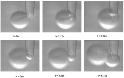
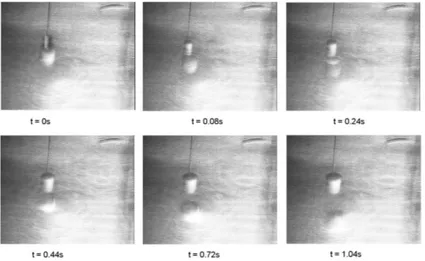
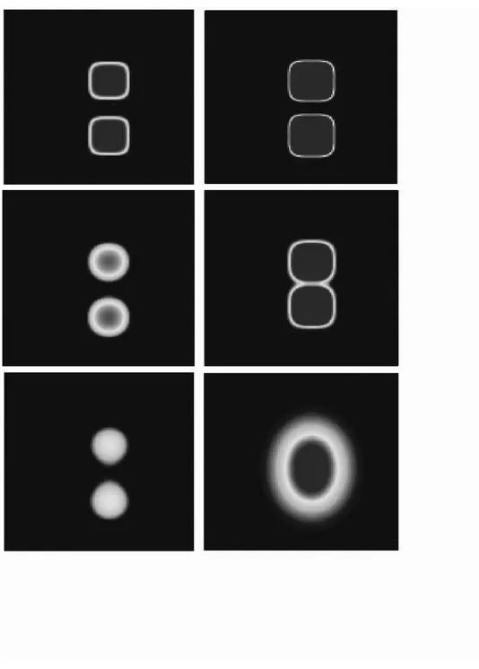
During the three years of the PhD project we extended the diffuse interface (DI) method and apply it to engineering related problems, particularly re-lated to mixing and demixing of two fluids. To do that, first the DI model itself was validated, showing that, in agreement with its predictions, a single drop immersed in a continuum phase moves whenever its composition and that of the continuum phase are not at mutual equilibrium [D. Molin, R. Mauri, and V. Tricoli, ”Experimental Evidence of the Motion of a Single Out-of-Equilibrium Drop,” Langmuir 23, 7459-7461 (2007)]. Then, we de-veloped a computer code and validated it, comparing its results on phase separation and mixing with those obtained previously. At this point, the DI model was extended to include heat transport effects in regular mixtures In fact, in the DI approach, convection and diffusion are coupled via a nonequi-librium, reversible body force that is associated with the Kortweg stresses. This, in turn, induces a material flux, which enhances both heat and mass transfer. Accordingly, the equation of energy conservation was developed in detail, showing that the influence of temperature is two-folded: on one hand, it determine phase transition directly, as the system is brought from the single-phase to the two-phase region of its phase diagram. On the other hand, temperature can also change surface tension, that is the excess free en-ergy stored within the interface at equilibrium. These effects were described using the temperature dependence of the Margules parameter. In addition, the heat of mixing was also taken into account, being equal to the excess free energy. [D. Molin and R. Mauri, ”Diffuse Interface Model of Multiphase Fluids,” Int. J. Heat Mass Tranf., submitted]. The new model was applied to study the phase separation of a binary mixture due to the temperature quench of its two confining walls. The results of our simulations showed that, as heat is drawn from the bulk to the walls, the mixture phase tends to phase separate first in vicinity of the walls, and then, deeper and deeper within the bulk. During this process, convection may arise, due to the above mentioned non equilibrium reversible body force, thus enhancing heat transport and, in particular increasing the heat flux at the walls [D. Molin, and R. Mauri, ”Enhanced Heat Transport during Phase Separation of Liquid Binary Mix-tures,” Phys. Fluids 19, 074102-1-10 (2007)]. The model has been extended then and applied to the case where the two phases have different heat

(4)

con-ductivities. We saw that heat transport depends on two parameters, the Lewis number and the heat conductivity ratio. In particular, varying these parameters can affect the orientation of the domains that form during phase separation. Domain orientation has been parameterized using an isotropy coefficient ξ, varying from -1 to 1, with ξ = 0 when the morphology is isotropic, ξ = +1 when it is composed of straight lines along the transversal (i.e. perpendicular to the walls) direction, and ξ = −1 when it is composed of straight lines along the longitudinal (i.e. parallel to the walls) direction [D. Molin, and R. Mauri, ”Spinodal Decomposition of Binary Mixtures with Composition-Dependent Heat Conductivities,” Int. J. Engng. Sci., in press (2007)]. In order to further extend the model, we removed the constraint of a constant viscosity, and simulated a well known problem of drops in shear flows. There we found that, predictably, below a certain threshold value of the capillary number, the drop will first stretch and then snap back. At lager capillary numbers, though, we predict that the drop will stretch and then, eventually, break in two or more satellite drops. On the other hand, applying traditional fluid mechanics (i.e. with infinitesimal interface thick-ness) such stretching would continue indefinitely [D. Molin and R. Mauri, ” Drop Coalescence and Breakup under Shear using the Diffuse Interface Model,” in preparation]. Finally, during a period of three months at the Eindhoven University, we extended the DI model to a three component fluid mixture, using a different form of the free energy, as derived by Lowengrub and Coworkers.. With this extension, we simulated two simple problems: first, the coalescence/repulsion of two-component drops immersed in a third component continuum phase; second, the effect of adding a third component to a separated two phase system. Both simulations seem to capture physical behaviors that were observed experimentally [D. Molin, R. Mauri and P. Anderson, ” Phase Separation and Mixing of Three Component Mixtures,” in preparation].

(5)

Introduction

The theory of multiphase systems was developed at the beginning of the 19th century by Young, Laplace and Gauss, assuming that different phases are separated by an interface, that is a surface of zero thickness. In this ap-proach, physical properties such as density and concentration, may change discontinuously across the interface and the magnitude of these jumps can be determined by imposing equilibrium conditions at the interface. For ex-ample, imposing that the sum of all forces applied to an infinitesimal curved interface must vanish leads to the Young-Laplace equation, stating that the difference in pressure between the two sides of the interface (where each phase is assumed to be at equilibrium) equals the product of surface tension and curvature. Later, this approach m was generalized by defining surface thermodynamical properties, such as surface energy and entropy, and surface transport quantities, such as surface viscosity and heat conductivity, thus formulating the thermodynamics and transport phenomena of multiphase systems. At the end of the 19th century, though, another approach was proposed by Rayleigh (1892) and Van der Waals (1893), who assumed that interfaces have a non-zero thickness, i.e. they are ”diffuse”. Actually, the ba-sic idea was not new, as it dated back to Maxwell (1876) and Gibbs (1876), Poisson (1831) and Leibnitz (1765) or even Lucretius (50 B.C.E.), who wrote that ”a body is never wholly full nor void.” Concretely, in a seminal article published in 1893, Van der Waals used his equation of state to predict the thickness of the interface, showing that it becomes infinite as the critical point is approached. Later, in 1901, Korteweg continued this work and pro-posed an expression for the capillary stresses, which are generally referred to as Korteweg stresses, showing that they reduce to surface tension when the region where density changes from one to the other equilibrium value col-lapses into a sharp interface (see Rowlinson and Widom, 1982, for a review of the molecular basis of capillarity). In the first half of the 20th century, the diffuse interface (D.I.) approach was basically ignored because assum-ing that interfaces are sharp allows one to obtain a few analytical results and seemed to better fit the needs of the multiphase scientific community. However, at mid 1900, Cahn and Hillard (again the Dutch school!) first ap-plied Van der Waals’ D.I. approach to binary mixtures (Cahn and Hillard, 1958) and then used it to describe nucleation (Cahn and Hillard, 1959) and

(8)

spinodal decomposition (Cahn, 1961). This approach was later extended to model spinodal decomposition of polymer blends and alloys (de Gennes, 1980; Pincus, 1981). Then, in the mid 1980’s, the D.I. approach was coupled to hydrodynamics, developing a set of conservation equations, thanks to the work by Kawasaki (1970), Siggia (1979), Hohenberg and Halperin (1977) and others. These latter authors referred to this approach as ”model H” and only later the name ”diffuse interface method” was introduced. Finally, recent development in computing technology has stimulated a resurgence of the D.I. approach, above all in the study of systems with complex morpholo-gies and topological changes. Detailed discussion about D.I. theory coupled with hydrodynamics can be found in Antanovskii (1996), Lowengrub and Truskinovsky (1997) and Anderson, McFadden and Wheeler (1998). In or-der to better unor-derstand the basic idea unor-derlying the D.I. theory, let us remind briefly the classical approach to multiphase flow that is used in fluid mechanics. There, the equation of conservation of mass, momentum, energy and chemical species are written separately for each phase, assuming that temperature, pressure, density and composition of each phase are equal to their equilibrium values. Accordingly, these equations are supplemented by boundary conditions at the interface, namely (see for example Davis and Scriven, 1982),

|∆τ |−₊· n = κσn; (1)

|∆v|−₊= 0, (2)

with n denoting the normal at the interface, stating that the jump of the stress tensor at the interface is related to the product of the curvature and the surface tension , while velocity v and temperature T are continuous (unless we introduce concepts such as surface viscosity and surface heat conductivity, so that they become discontinuous as well). Naturally, this results in a free boundary problem, which means that one of the main prob-lems of this approach is to determine the position of the interface. To that extend, many interface tracking methods have been developed, which have proved very successful in a wide range of situations. However, there are few instances where the interface tracking breaks down. That happens when the interface thickness is comparable to the lengthscale of the phenomenon that is being studied, such as a) in near-critical fluids or partially miscible mixtures, as the interface thickness diverges at the critical point; b) near the contact line along a solid surface or in the breakup/coalescence of liquid droplets, as the related physical processes act on lengthscales that are com-parable to the interface thickness. In addition, interface tracking becomes very problematic for self intersecting free boundaries. In front of these dif-ficulties, the D.I. method offers an alternative approach. Quantities that in the free boundary approach are localized in the interfacial surface, here

(9)

are assumed to be distributed within the interfacial volume. For example, surface tension is the result of distributed stresses within the interfacial re-gion, which are often called capillary, or Korteweg, stresses. In general, the interphase boundaries are considered as mesoscopic structures, so that any material property varies smoothly at macroscopic distances along the in-terface, while the gradients in the normal direction are steep. Accordingly, the main characteristic of the D.I. method is the use of an ”order parame-ter” which undergoes a rapid but continuous variation across the interphase boundary, while it varies smoothly in each bulk phase, where it can even assume constant equilibrium values. For a single-component system, the order parameter is the fluid density ρ, for a liquid binary mixture it is the molar (or mass) fraction φ, while in other cases it can be any other param-eter, not necessarily with any physical meaning, that allows to reformulate free boundary problems. In all these cases, the D.I. model must include a characteristic interface thickness, over which the order parameter changes. In fact, in the asymptotic limit of vanishing interfacial width, the diffuse in-terface model reduces to the classical free boundary problem. In Chapter 1 we formulate the diffuse interface model for single-component fluids and liq-uid binary mixtures at equilibrium, respectively. Then, in the next sections, the equations of motion are developed for non-dissipative systems, while at the end these results are generalized to the model dissipative systems. In Chapter 2, we presents some theory about the implementation of the model in and in Chapter 3 some results of numerical simulations are presented for the case of regular liquid binary mixtures, in particular in the first section is described an experimental result that it is used to validate the theoret-ical finding, in section two a validation of the code is presented based on reproducing the numerical results already published by Valdimirova et al. previously.

(10)

(11)

Chapter 1

Diffuse Interface Model

Reproduced in part from

”Diffuse Interface Model of Multiphase Fluids” D. Molin and R. Mauri,

Int. J. Heat Mass Tranf., submitted.

1.1 The free energy and Van der Waals’ equation

All thermodynamical properties can be determined from the Helmholtz free energy. This, in turn, depends on the intermolecular forces which, in a dense fluid, are a combination of weak and strong forces. Fortunately, strong interactions nearly balance each other, so that the net forces acting on each molecule are weak and long-range. In addition, mean field approximation is assumed to be applicable, meaning that molecular interactions are smeared out and can be replaced by the action of a continuous effective medium (see discussion in Pismen, 2001). Based on these assumptions, the case of dense fluids can be treated as that of nearly ideal gases, so that, allowing for variable density, the molar Helmholtz free energy at constant temperature

T can be written as (Landau & Lifshitz, 1980, Ch. 74): f [ρ(x)] = f_id+ 1 2RT NA Z ³ 1 − eU (r)/kT ´ ρ(x + r)d3r, (1.1) where k is Boltzmann’s constant, R = NAk is the gas constant, with NAthe Avogadro number, U is the pair interaction potential, which depends on the distance r = |r|, ρ is the molar density, while the factor 1/2 compensates counting twice the interacting molecules. The first term on the RHS,

f_id= RT ln ρ, (1.2)

is the molar free energy of an ideal gas (where molecules do not interact). Now, we assume that the interaction potential consists of a long-range term,

(12)

decaying as r−6 _{(like in the Lennard-Jones potential), while the short-range} term is replaced by a hard-core repulsion, i.e. (see Israelachvili, 1992)

U (r) =

(

−U₀(r/l)6 _{(r > d)}

∞ (r < d) (1.3)

where d is the nominal hard-core molecular diameter, l is a typical inter-molecular interaction distance, and the non-dimensional constant U0

rep-resents the strength of the intermolecular potential. When the density is constant, Eq. (1.1) gives the thermodynamic free energy, f_{T h},

fT h(T, ρ) = fid(T, ρ) + fex(T, ρ), (1.4) where

fex(T, ρ) = RT ρB(T ), (1.5) is the excess (i.e. the non ideal part) of the free energy, with

B(T ) = 1

2NA Z _∞

0

(1 − e−U (r)/kT)4πr2dr (1.6) denoting the first virial coefficient. This integral can be solved as:

B(T ) = 2πNA Z _d 0 r2dr + 2πNA Z _∞ d (1 − eU0kT(l/r)6)r2dr = b − a RT (1.7) where b = 2 3πd 3_N A (1.8)

is the excluded molar volume and

a = 2

3πU0N

2

Al6/d3 (1.9)

is a pressure adding term. Finally we obtain:

f_{T h}(ρ, T ) = f_id+ RT bρ − aρ ≈ RT ln µ ρ 1 − bρ ¶ − aρ, (1.10) that is fT h(ρ, T ) = RT ln(v − b) −a_v, (1.11) where v = ρ−1 is the molar volume. At this point, applying the thermody-namic equality (Landau & Lifshitz, 1980, Ch. 76) P = −(∂f /∂v)N,T, we obtain van der Waals’equation,

³

P + a v2

´

(13)

1.1.1 The critical point

In the P −T diagram, the vapor-liquid equilibrium curve stops at the critical point, characterized by a critical temperature TC and a critical pressure PC. At higher temperatures, T > TC and pressures, P < PC, the differences between liquid and vapor phases vanish altogether and we cannot even speak of two different phases In addition, as the critical point is approached, the difference between the specific volume of the vapor phase and that of the liquid phase decreases, until it vanishes at the critical point. Accordingly, near the critical point, since the specific volumes of the two phases, v and

v + δv , are near to each other, we obtain: P (T, v) = P (T, v + δv) = P (T, v) + µ ∂P ∂v ¶ T δv +1 2 µ ∂2_P ∂v2 ¶ T (δv)2+ ...., (1.13) where we have considered that the two phases at equilibrium have the same pressure, in addition of having the same temperature. At this point, dividing by v and letting δv → 0, we see that at the critical point we have:

µ ∂P ∂v ¶ T = 0, that is κT → ∞ as T → TC, (1.14)

where κT is the isothermal compressibility. Note that this condition is the limit case of the inequality (∂P/∂v)T ≤ 0, which manifests the internal stability of any single-phase system. In addition, since near an equilibrium point, δf + P δv > 0, expanding δf in a power series of δv, with constant T , we obtain: δfT h = µ ∂fT h ∂v ¶ T (δv) + 1 2! µ ∂2_f T h ∂v2 ¶ T (δv)2+ 1 3! µ ∂3_f T h ∂v3 ¶ T (δv)3 + 1 4! µ ∂4_f T h ∂v4 ¶ T (δv)4+ ...

Finally, considering that (∂fT h/∂v)T = −P and that at the critical point (∂2_f T h/∂v2)T = 0, we obtain: 1 3! µ ∂2_P ∂v2 ¶ TC (δv)3+ 1 4! µ ∂3_P ∂v3 ¶ TC (δv)4+ ... < 0. (1.15)

Since this equality must be valid for any value (albeit small) of δv (both positive and negative), we obtain:

µ ∂2_P ∂v2 ¶ TC = 0; µ ∂3_P ∂v3 ¶ TC < 0. (1.16)

(14)

Therefore, the critical point corresponds to a horizontal inflection point in the P − v diagram, which means that, since P = −(∂fT h/∂v)T,

µ ∂2_f T h ∂v2 ¶ TC = 0; µ ∂3_f T h ∂v3 ¶ TC = 0. (1.17)

Imposing that at the critical point the P −v curve has a horizontal inflection point, we can determine the constant a e b in the Van der Waals equation (the same is true for any 2 parameter cubic equation of state) in terms of the critical constant TC and PC, finding (Landau & Lifshitz, 1980, Ch. 84):

a = 9 8RTCvC = 27 64 (RT_C)2 PC and b = 1 3vC = 1 8 RT_C PC . (1.18) Viceversa, the critical pressure, temperature and volume can be determined as functions of a and b as follows:

P_C = 1 27 a b2; TC = 8 27 a Rb; vC = 3b; ZC = PCvC RT_C = 3 8 = 0.375. (1.19) Note that, imposing that PCvC = (3/8)RTC and substituting the expressions for a and b in terms of the intermolecular potential, we obtain the following

relation: _µ l d ¶₂ = 3 2 µ kTC U0 ¶_1/3 (1.20) Using these expressions, the Van der Waals equation can be written in terms of the reduced coordinates as:

µ Pr+_v3₂ r ¶ (3vr− 1) = 8Tr; Pr = _PP C ; vr = _vv C ; Tr= _TT C . (1.21)

This equation represents a family of isotherms in the Pr−vrplane describing the state of any substance, which is the basis of the law of corresponding states. As expected, when Tr > 1, the isotherms are monotonically decreas-ing, in agreement with the stability condition (∂P/∂v)T < 0, while when

Tr < 1, each isotherm has a maximum and a minimum point and between them we have an instability interval, with (∂P/∂v)_T > 0, corresponding to

the two-phase region (see Figure 1.3).

1.1.2 Coexistence and spinodal curves

Let us consider a one-component system at equilibrium, whose pressure and temperature are below their critical values, so that it is separated into two coexisting phases, say α and β. According to the Gibbs phase rule, these two phases have the same pressure and temperature and therefore, defining the Gibbs molar free energy g_{T h} = f_{T h} + P v, with dg_{T h} = −sdT + vdP ,

(15)

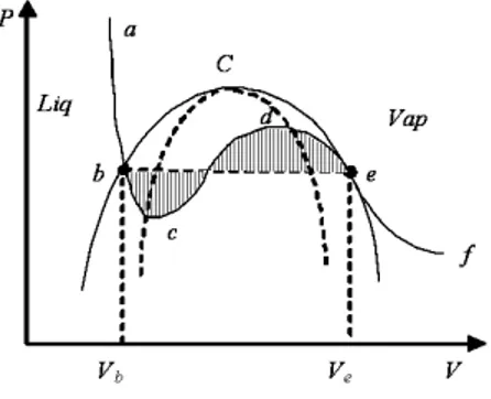
Fig. 1.1: Phase diagram (P − v) of a single component fluid and (µ − φ) of a binary mixture.

the corresponding equilibrium, or saturation, pressure P_sat at a given tem-perature can be easily determined from the equilibrium condition, stating that at equilibrium the Gibbs molar free energies of the two phases must be equal to each other. So we obtain:

gβ_{T h}− gα_{T h} = Z _e b dg_{T h} = 0 =⇒ Z _e b vdP = Z _e b v µ δP δv ¶ T dv = 0, (1.22)

where P = P (v) represents an isotherm transformation. From a geometrical point of view, this relation manifests the equality between the shaded area of Figure 1.1 (Maxwell’s rule), where the point b and e correspond to the equilibrium, or saturation, point of the liquid and vapor phases at that temperature at equilibrium, respectively, with specific volumes vα

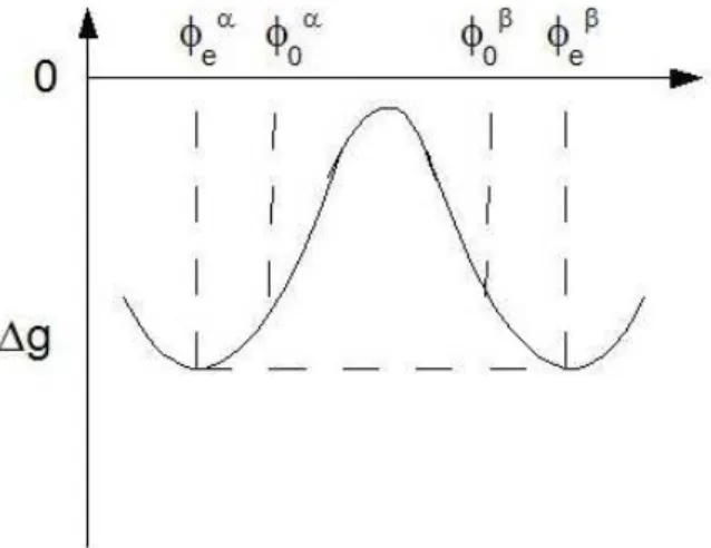
e and veβ. Conversely, the specific volumes of the two phases at equilibrium could also be determined from the molar free energy fT h, rewriting Eq. (1.20) in terms of reduced coordinates as fT h RTC = Trln(vC) − Trln µ vr−1₃ ¶ − 9 8vr. (1.23) When Tr < 1, a typical curve of the free energy is represented in Figure 1.2. Now, keeping Tr fixed and considering that the two phases at equi-librium have the same pressure, using the relation P = −(∂f_{T h}/∂v)_T , we obtain: Pα= Pβ =⇒ µ ∂f_th ∂v ¶_α T = µ ∂f_{T h} ∂v ¶_β T , (1.24)

which, in Figure 1.2, represents the fact that the two equilibrium points have the same tangent. From this relation we can determine the specific

(16)

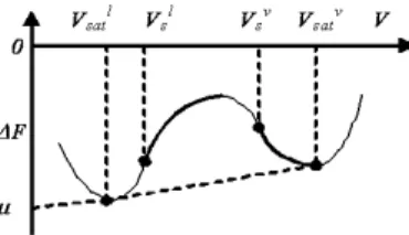
Fig. 1.2: Typical double-well curve of the free energy of a single component fluid.

volumes of the two phases at equilibrium, vα

e and vβe. This relation can also be obtained considering that the specific volumes of the two phases at equilibrium minimizes the total free energy, i.e.

F_{T h}= Z

ˆ

f_{T h}(ρ)d3x = min., (1.25) where ˆf = ρf is the free energy per unit volume,

ˆ

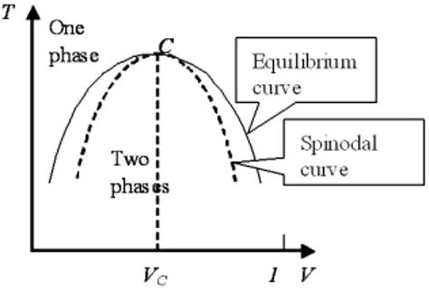
f_{T h} = ρf_{T h}= ˆf_id+ ˆf_ex = RT [ρ ln ρ + ρ2B(T )]. (1.26) This minimization is carried over in Section 1.1.5. In Figure 1.1, besides the equilibrium curve, we have represented the, so called, spinodal curve, defined as the locus of all points (like c and d) satisfying (∂P/∂v)T = 0. When the equilibrium and spinodal points are plotted in a T − v diagram, we obtain the curves of Figure 1.3.

All points lying outside the region encompassing the equilibrium curve are stable and represent homogeneous, single-phase systems; all points lying inside the region within the bell-shaped spinodal curve are unstable and represent systems that will separate into two phases (one liquid and another vapor, in this case); the region sandwiched between the equilibrium and the spinodal curves represents metastable systems, that is overheated liquid and undercooled vapor. The spinodal points can be also determined using the relation (∂P/∂v)_T = 0, obtaining: µ ∂2_f T h ∂v2 ¶ T = 0, (1.27)

determining the spinodal specific volumes ˜vα

(17)

Fig. 1.3: Phase diagram (T − v) of a single component fluid and (T − φ) of a binary mixture.

1.1.3 The critical exponents

Let us turn now to study the equation of state of a single component system close to its critical point. Then, instead of T , P and v, it is convenient to use the following variables:

˜t ≡ Tr− 1 = T − T_T C C ; ˜p ≡ Pr− 1 = P − PC PC ; ˜v ≡ vr− 1 = v − vC vC , (1.28) where Tr = T /TC, Pr = P/PC and vr = v/vC are the reduced variables. At the end of a tedious, but elementary power expansion in terms of these variables, we see that the Van der Waals equation reads, neglecting higher order terms,

˜

p = 4˜t− 5˜t˜v −3

2v˜

3_. _(1.29)

Note that we cannot have any term proportional to ˜v or ˜v2, in agreement with the conditions (∂P/∂˜v)TC = (∂2P/∂˜v2)TC = 0, while the coefficient

of the ˜v3_{-term must be negative, as (∂}3_P/∂˜_v3₎

TC < 0. When ˜t > 0, all

states of the system are stable, that is there is no phase separation and the system remains homogeneous. That means that, when ˜t > 0, it must be (∂P/∂˜v)TC < 0, and therefore the coefficient of the ˜t˜v-term must be negative.

Finally, note that the ˜t˜v2 and ˜t2˜v-terms have been neglected because they

are much smaller than ˜t˜v, while the ˜t˜v-term must be kept, despite being

much smaller than ˜t, for reasons that will be made clear below. In general, in the vicinity of the critical point the isotherms of a homogeneous system can be written as

˜

(18)

This expression for the free energy is the basis of Landau’s mean field theory (Landau & Lifshitz, 1980, Ch. 146, 148); it corresponds to Van der Waals’ Eq. (1.29) with ac= 3, bc= 4 and Bc= 3/8. At the critical point, where ˜t = 0 , from (1.30) we obtain: ˜p ∝ ˜vδ_{, where δ = 3 is a critical exponent, that we} find unaltered in all critical phenomena. Following an isotherms ˜t = costant, in the unstable region between the spinodal points, where (∂P/∂v)T > 0, the system separates into two coexisting phases. At equilibrium, the two specific volumes satisfy Eq. (1.24), and considering that

µ ∂ ˜p ∂˜v ¶ ˜ t = −2ac˜t− 12Bc˜v2, (1.31) we can determine the specific volumes of the two phases at equilibrium:

˜ vα_e = −˜vβ_e = s −aC˜t 2B ⇒ ∆˜v αβ e = ˜veα− ˜vβe ∝ (−˜t)β, (1.32) where β = 1/2 is another critical exponent. Now we see why we could not neglect the ˜v˜t term: if we did it, the two specific volumes would result

equal to each other. Note that the difference between the specific volumes of points that lye on the spinodal curve can be determined as well, applying the condition (∂ ˜p/∂˜v)_T_˜ = 0, obtaining:

˜

v_sα= −˜v_sβ = s

−ac˜t

6Bc . (1.33)

The critical properties can also be determined from the free energy fT h. In fact, integrating (df_{T h})_T = −P dv and substituting (1.30), we see that in the vicinity of the critical point the free energy has the following expression:

fT h(˜v, ˜T ) = PCvC[h( ˜T ) + (1 + bcT )˜˜ v + acT ˜˜v2+ Bcv˜4], (1.34) where h(˜t) is an undetermined function of the temperature. For a Van der Waals system, we obtain the same result expanding (1.21); in that case,

h(˜t) = (1 + ˜t) ln[3/(2vC)] − 9/8. Finally, applying (1.24) and (1.27), we obtain again (1.32) and (1.33). Another critical exponent, γ , is defined as

κ−1_T ∝ ˜tγ , where κT is the isothermal compressibility coefficient. From its definition, we obtain: κ−1_T = −v µ ∂P ∂v ¶ T = −P_C(1 + ˜v) µ ∂ ˜p ∂˜v ¶ ˜ T ∼ = 2acPC˜t, (1.35) showing that γ = 1. On the equilibrium curve, with ˜t < 0 and ˜v = 0, we

have ˜p = b_c˜t [see Eq. (1.30)]. Therefore, applying the Clausius-Clapeyron

equation, µ dP dT ¶_sat = ∆hαβ T (vβ _{− v}α₎ =⇒ d ˜P d˜t = b ∼= ∆hαβ PCvC(˜vβ− ˜vα), (1.36)

(19)

where ∆hαβ _{is the latent heat of vaporization, we obtain an expression for} ∆hαβ near the critical point,

∆hαβ ∼= bcRTC(˜vβ− ˜vα) = s

acb2c

Bc RT

Cp_−˜t, _(1.37)

where we have substituted Eq. (1.32), considering that P_CV_C ∼= RTC. From this equation we see that on approaching the critical point the latent heat of evaporation vanishes like p−˜t.

Finally, the last thermodynamical quantity to be determined is the spe-cific heat. From the definition, cv = (∂uT h/∂T )V, where uT h is the molar internal energy, and considering that uT h = fT h+ T s = fT h− T (∂fT h/∂T )v, we obtain from Eq. (1.34)

csat_v = PCvC TC · 1 + b_c+ f_{T h}(0) −dfT h d˜t (0) ¸ . (1.38)

Therefore, we see that csat

v remains finite at the critical point and it does not depend on ˜t, that is cv ∝ ˜tα, where α = 0 is another critical exponent. Consequently, using the well known relation

cp− cv ∝ ·µ ∂ ˜p ∂˜t ¶ ˜ v ¸₂Á µ ∂ ˜p ∂˜v ¶ , (1.39)

we see that, since (∂ ˜p/∂˜t)_˜_t=0,˜_v=0 = b_c and (∂ ˜p/∂˜v)_˜_t=0,˜_v=0 = 0, the specific heat cp diverges. In fact, we find:

cp ∝ 1 (∂ ˜p/∂˜t)˜t = 1 −2ac˜t− 12Bc˜v2 ∝ 1 ˜t, (1.40)

where we have considered that on the equilibrium curve, ˜v ∝√˜t. It has been

shown (see Le Bellac, Ch. 1.3) that the mean field theory provides results that compare favorably with those that have been obtained by molecular dynamics simulations.

1.1.4 The diffuse interface

Suppose now that the molar density of the system is not constant. Accord-ingly, when U ¿ kT , Eq. (1.1) can be rewritten as

f (x) = f_{T h}(x) + ∆f_{N L}(x), (1.41) where fT h is the molar free energy (1.4) corresponding to a system with constant density, while

∆fN L(x) = 1₂NA2 Z

r>d

(20)

is a non local molar free energy, due to density changes, typical of the diffuse interface model. In fact, when there is an interface separating two phases at equilibrium, this term corresponds to the interfacial energy. This result is a direct consequence of the ”exact” expression (1.1), showing that the free energy is non-local, that is its value at any given point does not depend only on the density at that point, but it depends also on the density at neighboring points. As stated by Van der Waals (1893), ”the error that we commit in assuming a dependence on the density only at the point considered vanishes completely when the state of equilibrium is that of a homogeneous distribution of the substance. If, however, the state of equilibrium is one where there is a change of density throughout the vessel, as in a substance under the action of gravity, then the error becomes general, however feeble it may be.” Now, in (1.42) the density can be expanded as

ρ(x + r) = ρ(x) + r · ∇ρ +1

2rr : ∇∇ρ + .. (1.43) As we have tacitly assumed that the system is isotropic, we see that the contribution of the linear term vanishes, so that, at leading order, we obtain (Pismen, 2001): ∆fN L(x) = − 1 2RT K∇ 2_ρ(x), _(1.44) with K = 2π 3 NAU0 kT l6 d = 9π 4 TC T NAd 5_, _(1.45)

where we have substituted (1.20). Note that, defining a non-dimensional molar, ˜ρ = NAd3ρ , the non local free energy can be rewritten as

∆fN L(x) = −1₂RT a2∇2ρ(x),˜ (1.46) where a = r K N_Ad3 = r 9πTC 4T d (1.47)

is the characteristic length. The total free energy is therefore:

F =

Z V

ˆ

f dV d3x, (1.48) where ˆf = ρf is the free energy per unit volume. Now, observing that,

integrating by part, Z

ρ(x)∇2ρ(x)d3x = − Z

|∇ρ(x)|2d3x, (1.49) we see that the free energy per unit volume is:

ˆ f (ρ, ∇ρ, T ) = RT · ρ ˜fT h(ρ, T ) + 1 2K(T )(∇ρ) 2 ¸ = RT · ρ ln ρ + B(T )ρ2+ 1 2K(T )(∇ρ) 2 ¸ ,

(21)

where ˜f_{T h} = f_{T h}/RT . Now, at equilibrium, the total free energy F will be

minimized, subjected to the constraint of having a constant number of moles, R

ρd3_{x = const. Accordingly, introducing a Lagrange multiplier, RT ˜}_{µ, the}

minimization condition is:

δ Z (ρf − RT ˜µρ)d3x = 0, (1.50) that is, δ Z ρ(x)[ ˜fT h[ρ(x)] − ˜µ] +1₂K|∇ρ(x|2)d3x = 0. (1.51)

1.1.5 The generalized chemical potential

The Euler-Lagrange equation corresponding to the minimization condition (1.51) is (see derivation in Section 1.2.5):

˜ µ = 1 RT δ(ρ ˆf ) δρ = d(ρ ˜f_{T h}) dρ − K∇ 2_ρ. _(1.52)

Now, by definition, RT ˜µ = f_{T h}− v(∂f_{T h}/∂v)_T is Gibbs free energy, which, in a one-component system, coincides with the chemical potential, i.e.,

˜

µ_{T h} = d(ρ ˜fT h)

dρ = ˜fT h− v d ˜f_{T h}

dv . (1.53)

This (apart from the dimensional constant RT ) is the equation of the straight line represented in Figure 1.2, stating that two phases at mutual equilibrium have the same chemical potential. Therefore, Eq. (1.52) can be rewritten as

˜

µ(ρ, ∇ρ) = ˜µT h(ρ) − K∇2ρ, (1.54) showing that at equilibrium, when ρ is non-uniform, it is ˜µ, and not ˜µT h, that remains uniform. Note that the thermodynamic chemical potential, ˜

µT h, can be determined from the solvability condition of Eq. (1.53), that is:

˜ µT h = ρα_f˜α T h− ρβf˜T hβ ρα_{− ρ}β = vα_f˜α T h− vβf˜T hβ vα_{− v}β , (1.55) as it can also be seen geometrically from Figure 1.2, stating that the chemical potential equals the intercept of the tangent line on the v = 0 vertical axis. Accordingly, as at the critical point this tangent line becomes horizontal, there the chemical potential must vanish [this result can also be obtained from Eq. (1.32) and (1.34)]. When two phases are coexisting at equilibrium, separated by a planar interfacial region centered on z = 0, Eq. (1.52) can be solved once the equilibrium molar free energy f is known, imposing that, far from the interface region, the density is constant and equal to its

(22)

equilibrium value, so that the generalized chemical potential is equal to its thermodynamic value (1.53). In particular, in the vicinity of the critical point, the chemical potential vanishes, the free energy is given by Eq. (1.34) and we obtain at leading orders the following equation:

d2_v_˜

d˜z2 − 2a˜t˜v − 4B˜v3 = 0, z = z/λ;˜ λ =

s

K

v_C(−a˜t), (1.56) to be solved imposing that

˜

v(˜z −→ ±∞) = ±˜ve= ± s

−a˜t

2B. The solution, due (again!) to Van der Waals (1893), is:

˜

v(˜z) = ˜vetanh ˜z, (1.57) showing that λ is a typical interfacial thickness. For a Van der Waals system, considering that K is given by Eq. (1.45), v_C = 3b = 6πd3_N

A and a = 3, we obtain: λ = s A 27(−˜t) l3 d2 = s 1 8(−˜t)d, (1.58)

where we have substituted Eq. (1.20). As expected, the interfacial thickness diverges like (−˜t)−1/2 _{as we approach the critical point, while far from the} critical point it is of O(d). Recently, Pismen (2001) pointed out that Eq. (1.56) is flawed, as some of the neglected terms diverge at the critical point. In fact, Pismen showed that in the correct solution the specific volume tends to its equilibrium value as |z|−4_{, instead of exponentially, as in the Van der} Waals solution.

1.1.6 The surface tension

In the previous section we have seen that the total free energy is the sum of a thermodynamical, constant density, part, and a non local contribution (1.42). When the system is composed of two phases at equilibrium, separated by a plane interfacial region, we may define the surface tension as the energy per unit area stored in this region. This quantity can be calculated through the following integral:

σ = −1 2RT K Z _∞ −∞ ρd2ρ dz2dz = 1 2RT K Z _∞ −∞ µ dρ dz ¶₂ dz, (1.59)

where we have integrated by parts and considered that, outside the interfa-cial region, the integrand is identically zero as density is constant. We see that, near the critical point,

(23)

where we have considered Eqs. (1.32), (1.45) and (1.58). In fact, using the density profile (1.57), Eq. (1.59) yields, for a Van der Waals system:

σ = 2 3RTC(−a˜t) 3/2 µ K v3 c ¶ = CkTC d2 (−˜t)3/2, (1.61)

with C = 33/2_/(23/2_{π), where we have used Eq. (1.20). These results}

show that the surface tension decreases as we approach criticality, until it vanishes at the critical point. A more detailed numerical solution based on the solution of the Van der Waals equation can be found in Pismen and Pomeau (2000). Applying this approach, Van der Waals (1893) showed that in a curved interface region there arises a net force [see Section 1.3.1], which is compensated by a pressure term, thus obtaining the Young-Laplace equation. To see that, let us denote the position of the interface by z = h(ξ), where ξ is the 2D vector in the support plane, and assume that |∇ξh| ¿ 1, where |∇_ξh| is the 2D gradient (see Pismen, 2001). Now, the free energy

increment due to the interface curvature can be written as ∆F = σ Z µq 1 + |∇ξh|2− 1 ¶ d2ξ ≈ 1 2σ Z |∇ξh|2d2ξ. (1.62) This increment is the free energy induces an increment in the pressure,

∆P = δF/δh = −σ∇2h = −κσ, (1.63) where κ = ∇2_{h is the curvature of a weekly curved interface. Applying a}

rigorous regular perturbation approach to Eq. (1.52), Pismen (2000) de-rived both the Young-Laplace equation (1.63) and the Gibbs-Thomson law, relating the equilibrium temperature or pressure to the interfacial curvature.

1.2 Binary mixtures

In this Section we will show that Van der Waals’ approach can be applied to study binary solutions. To simplify matters, at first let us confine ourselves to the case of regular binary solutions, that are mixtures in which the volume and the entropy of mixing are both equal to zero. That means that when we mix the two species, say 1 and 2, a) the volume remains unchanged, so that the mixture can be considered to be incompressible, and b) the entropy change is equal to that of ideal mixtures (see Sandler, 1999, Section 7.6). Generalization to non regular, even compressible, binary mixtures can be found in Lowengrub and Truskinovsky (1997).

1.2.1 The Gibbs free energy

The molar free energy can be determined using the same procedure as for single component systems. Consider a mixture composed of species 1 and

(24)

species 2, with molar fraction x1 = φ and x2 = (1 − φ) and let us first

determine the molar free energy when the composition of the mixture is uniform. Considering the definition of Gibbs free energy, g = f + P/ρ, from Eq. (1.1) we obtain:

gT h(φ) = gid(φ) + gex(φ). (1.64) Here gidis the Gibbs free energy of an ideal mixture, that is a mixture where the intermolecular potentials Uij between molecule i and molecule j are all the same, i.e. U₁₁ = U₂₂ = U₁₂. Generalizing the expression of the free energy for a single component fluid, RT ln ρ, we obtain:

g_id = RT [x₁ln(x₁ρ) + x₂ln(x₂ρ)],

that is:

gid= RT ln ρ + RT [φ log φ + (1 − φ) log(1 − φ)]. (1.65) Note that for a pure fluid the molar density ρ is a variable, while for a regular binary mixture the total molar density ρ can even be constant, since the variables are the molar densities of the two components, x₁ρ and x₂ρ.

The second term in the RHS of Eq. (3.44), gex, is the so called excess, that is non ideal, part of the free energy. This term has a particularly convenient form for regular mixtures, as it is explained below. The theory of regular mixtures was developed by Van Laar (a student of van der Waals), who assumed that (a) the two species composing the mixture are of similar size and energies of interaction, and (b) the Van der Waals equation of state applies to both the pure fluids and the mixture. Consequently, regular mixtures have negligible excess volume and excess entropy of mixing, i.e. their volume and entropy coincide with those of an ideal gas mixture, with

sex = 0 and vex = 0. Therefore, we see that for a regular mixture, since

s_ex = −(∂g_ex/∂T )_P,x= 0, then g_ex must be independent of T . In addition, as the excess Gibbs free energy results to be equal to the excess internal energy, i.e. gex = uex, it can be shown (see Sandler, 1999, Section 7.6) that the Gibbs free energy of a regular mixture with molar fractions x₁ and

x2 = 1 − x1 is: gex= x1a_b1 1 + x2 a2 b2 − amix bmix, (1.66)

where we have used obvious notations to indicate the Van der Waals con-stants (a and b) for the pure fluids, 1 and 2, and for the mixture, and we have considered that uex = a/b. From here, assuming that

bmix= b1 = b2; amix= x21a1+ x22a2+ 2x1x2a12, (1.67)

with a₁₂=√a₁a₂, we obtain,

(25)

Thus, we see again that the excess free energy does not depend on T , so that

sex = 0. Similar considerations can be applied to the dependence of the free energy on the pressure, confirming that vex = 0 for regular mixtures.

The same conclusions can be reached starting from the fundamental expression (1.1) for the Helmholtz free energy and considering that:

gex = fex+ P vex. (1.69) Applying Eq. (1.20) to a system with constant molar density ρ, i.e. with

vex= 0, we obtain: gex= fex= RT ρB, where B is the virial coefficient,

B = x2₁B₁₁+ 2x₁x₂B₁₂+ x₂B₂₂. (1.70) Here Bij characterizes the repulsive interaction between molecule i and molecule j [see Eq. (1.6)],

B_ij = 1 2NA Z · 1 − exp µ −Uij(r) kT ¶¸ d3r. (1.71) In particular, for symmetric solutions, U11 = U22 6= U12, so that B11 =

B₂₂6= B₁₂. Accordingly, denoting x₁= φ, we obtain:

gex= ρRT B = 2ρRT (B12− B11)φ(1 − φ),

that is,

gex(T, P, φ) = RT Ψ(T, P )φ(1 − φ), (1.72) where

Ψ(T, P ) = 2ρ(B12− B11), (1.73)

is the so called Margules coefficient (Sandler, 1999). In particular, for an ideal mixture, B11= B12 and therefore Ψ = 0. For a mixture composed of

Van der Waals fluids at constant pressure, substituting the expression (1.6) for B and assuming that the characteristic lengths d and l are the same for the two species, we obtain:

Ψ = 2ρ RT(a11− a12) = 4π 3 ρN2 Al6 RT d3(U0,11− U0,12), (1.74)

where U0,11 and U0,12 characterize the strength of the potential between

molecules of the same species and that of different species, respectively. From this expression we see that Ψ ∝ T−1, confirming that gex is independent of

T . Note that when Ψ > 0 the repulsive forces ∼= U0,12/d between unlike

molecules are weaker than those between like molecules, ∼= U0,11/d. As

shown in Mauri, Shinnar and Triantafyllou (1996), when the solution is not symmetric, this approach is easily generalized by defining two Margules coefficients.

(26)

1.2.2 Coexistence and spinodal curve

In the previous Section, we saw that the free energy of a homogenous sym-metric binary mixture can be written as:

gT h= g1+ RT [φ log φ + (1 − φ) log(1 − φ) + Ψφ(1 − φ)]. (1.75)

Now, the thermodynamic state of a one-component system is determined by fixing two quantities, e.g. P and T . In binary mixtures, we have an additional degree of freedom, i.e. the molar fraction of the two species, x1.

Associated with x1 and x2 we can define the respective chemical potentials,

RT µi = ∂(N gT h/Ni)j6=i. Generalizing the relation obtained in the previous Section, at equilibrium the chemical potentials µ1 and µ2 are uniform

every-where and, in particular, they must be the same in each phase, i.e. µα

1 = µβ1

and µα₂ = µβ₂. Considering that x1 and x2 depend on each other, there is a

relation between µ1 and µ2, namely the Gibbs-Duhem relation (see Sandler,

1999), x₁∇µ₁= −x₂∇µ₂. This relation can be easily obtained by imposing that the specific Gibbs free energy, gth, defined as,

N g_{T h} = N u_{T h}− N T s + N P v + RT N1µ1+ RT N2µ2, (1.76)

where uT h is the molar internal energy, must satisfy the following equality,

dgT h= −sdT + vdP + RT µdφ, (1.77) where µ = µ₁ − µ₂ is the chemical potential difference. This last relation reveals that the chemical potential difference is the quantity that is thermo-dynamically conjugated with the composition φ. This same result can be obtained from the identities (Sandler, 1999),

RT µ1(T, P, φ) = gT h(T, P, φ) + µ dgT h dφ ¶ (1 − φ), (1.78) RT µ2(T, P, φ) = gT h(T, P, φ) + µ dg_{T h} dφ ¶ φ, (1.79) obtaining, µ = µ1− µ2 = d(g_{T h/RT}) dφ = log µ φ 1 − φ ¶ + Ψ(1 − 2φ), (1.80)

where we have substituted Eq. (1.75). At constant temperature T and pres-sure P , since Ψ is a known function of T and P , this equation gives the dependence of the chemical potential difference on the composition, just like the equation of state, e.g. Van der Waals’ equation, gives the dependence of the pressure on the specific volume. Clearly, µ represents the tangent to the free energy curve and it is the same for the two phases at equilibrium.

(27)

Accordingly, this equation leads to the determination of the equilibrium composition of the two coexisting phases, φα_e and φβe. In particular, in our case, where we have considered symmetric mixtures, the tangent is horizon-tal and therefore µ = 0. Note that, as expected, in this case φα

e = 1 − φβe. Now we can apply to binary mixtures the same considerations about the critical point that we made in the previous Section on one-component sys-tems, observing that chemical potential difference µ and composition φ play the same role as pressure and density (or specific volume). In fact, in the

µ−T diagram, the liquid-liquid equilibrium curve stops at the critical point,

characterized by a critical temperature TC and a critical chemical potential difference, µ_C = 0 (note that for symmetric mixtures µ = 0 at any equilib-rium state, while in general that is true only at the critical point). At higher temperatures, T > TC, the differences between the two liquid phases vanish altogether and the system is always in a single phase. In addition, as the critical point is approached from below (i.e. with two coexisting phases), the difference between the composition of the two phases decreases, until it vanishes altogether at the critical point. Accordingly, near the critical point, since the composition of the two phases, φ and φ + δφ, are near to each other, we obtain (Landau and Lifshitz, 1980, Ch. 97):

0 = µ_C(T, φ) = µ_C(T, φ + δφ) =⇒ 0 = µ ∂µ ∂φ ¶ TC,PC δφ + 1 2 µ ∂2µ ∂φ2 ¶ TC,PC (δφ)2+ ....,

where we have considered that, since the two phases are at equilibrium, they have the same chemical potential (in addition to having the same pressure and temperature). At this point, dividing by δφ and letting ∂φ −→ 0, we see that at the critical point we have:

µ ∂µ ∂φ ¶ TC,PC = 0. (1.81)

Note that this condition is the limit case of the inequality (∂µ/∂φ)T,P ≤ 0, which manifests the internal stability of any two-phase system. In addition, expanding δg_{T h} in a power series of δφ, with constant T and P , we obtain:

δgT h = µ ∂gT h ∂φ ¶ T,P (δφ) + 1 2! µ ∂2_g T h ∂φ2 ¶ T,P (δφ)2+ 1 3! µ ∂3_g T h ∂φ3 ¶ T,P (δφ)3 + 1 4! µ ∂4_g T h ∂φ4 ¶ T,P (δφ)4+ ..

Therefore, since near an equilibrium point, we have:

(28)

considering that (∂g_{T h}/∂φ)T,P = RT µ and that at the critical point (∂ 2_g T h ∂φ2 )T,P = 0, we obtain: 1 3! µ ∂2_µ ∂φ2 ¶ TC,PC (δφ)3+ 1 4! µ ∂3_µ ∂φ3 ¶ TC,PC (δφ)4+ .. > 0. (1.82) Since this equality must be valid for any value (albeit small) of ∂φ (both positive and negative), we obtain:

µ ∂2_µ ∂φ2 ¶ TC,PC = 0; µ ∂3_µ ∂φ3 ¶ TC,PC > 0. (1.83)

Therefore, the critical point corresponds to a horizontal inflection point in the µ − φ diagram (see Figure 1.1), which means that,

µ ∂2gT h ∂φ2 ¶ TC,PC = 0; µ ∂3gT h ∂φ3 ¶ TC,PC = 0. (1.84)

Imposing that at the critical point the µ−φ curve has a horizontal inflection point, from Eq. (1.80) we see that φα

C = φβC = 1/2, confirming that ΨC = 2. Therefore, considering that Ψ ∝ T−1_{, we obtain:}

Ψ = 2TC

T (1.85)

In particular, near the critical point, defining ˜ψ = (Ψ − 2)/2 and ˜t = (T_C− T )/TC, we obtain at leading order:

˜

ψ = −˜t. (1.86)

Now, let us consider a binary liquid mixture at equilibrium, whose chemical potential difference and temperature are below their critical values, so that the mixture is separated into two coexisting phases. At equilibrium, the phase transition takes place at constant temperature, pressure and chemi-cal potential difference and therefore it can be represented as a horizontal isotherm isobaric segment in a µ − φ diagram. Now, define a generalized potential (see Landau and Lifshitz, 1980, Ch. 85) as Φ_{T h} = g_{T h}− µφ, with dΦT h = −sdT + vdP − RT φdµ and (∂Φ/∂µ)T,P = RT φ. The chemical potential difference µ at a given temperature and pressure can be easily de-termined, considering that at equilibrium the generalized potentials of the two phases must be equal to each other, that is

Φβ_{T h}− Φα_{T h} = Z _e b dΦT h = 0 ⇒ Z _e b φdµ = Z _e b φ µ ∂µ ∂φ ¶ T,P dφ = 0, (1.87)

where we have considered that the phase transition is isothermal and iso-baric. From a geometrical point of view, this relation manifests the equality

(29)

Fig. 1.4: Typical double-well curve of the free energy of a symmetric binary mixture.

between the shaded area of Figure 1.1 (Maxwell’s rule), where the point b and

e correspond to the saturation points of the two phases at that temperature

and pressure, with compositions φα _{and φ}β_{. Conversely, the composition of} the two phases at equilibrium can be determined from the molar free en-ergy g of Eq. (1.75) as follows. A typical curve of the free enen-ergy g for a symmetric binary mixture is represented in Figure 1.4, when T < T_C (i.e. when Ψ > 2). The condition (1.87) expresses the fact that at equilibrium the two phases have the same temperature, pressure and chemical potential (so that the chemical potential difference µ is identically zero). Being on an isotherm-isobar, the first two conditions are automatically satisfied while, using the relation µ = (∂g/∂φ)T,P, the last condition gives:

µα = µβ = 0 =⇒ µ ∂g_{T h} ∂φ ¶_α T,P = µ ∂g_{T h} ∂φ ¶_β T,P =⇒ (φα_e, φβ_e), (1.88) which, in Figure 1.4, represents the fact that the two equilibrium point have the same tangent and this tangent is a horizontal line. When the mixture is not symmetric, the gT h − φ curve is similar to the fT h− v curve of Figure 1.2. Consequently, it is still true that µα _{= µ}β_{, but, in general, they are} not equal to zero, i.e. the tangent to the Gibbs free energy curve is not horizontal.

In Figure 1.1, besides the equilibrium curve, we have represented the, so called, spinodal curve, defined as the locus of all points (like c and d)

(30)

satisfying (∂µ/∂φ)T,P = 0. When the equilibrium and spinodal points are plotted in a T − φ diagram (at constant pressure), we obtain the curves of Figure 1.3. All points lying outside the region encompassing the equilib-rium curve represent homogeneous, single-phase mixtures in a state of stable equilibrium, while all points lying inside that region represent systems in a state of non equilibrium, which tend to separate into two phases. How-ever, all points lying in the region inside the spinodal curve are unstable, that is any infinitesimal perturbation can trigger the phase transition pro-cess, while all points sandwiched between the equilibrium and the spinodal curves represent metastable systems, i.e. mixtures that need an activation energy to phase separate. The spinodal points can be also determined using the relation (∂µ/∂φ)T,P = −(∂2gT h/∂φ2)T,P = 0 , obtaining:

µ ∂2gT h ∂φ2 ¶ T,P = 0 =⇒ (φα_s, φβ_s). (1.89)

1.2.3 The critical exponents

Let us turn now to study the behavior of a binary mixture close to its critical point. Then, instead of Ψ and φ, it is convenient to use the following variables,

˜

ψ = 1

2(Ψ − 2); u = 2φ − 1.˜ (1.90) Consequently, neglecting higher order terms, we obtain from the equation of state (1.80),

µ = −2 ˜ψ˜u +2

3u˜

3_. _(1.91)

Note that we cannot have any term proportional to ˜u or ˜u2_{, in agreement}

with the conditions (∂µ/∂φ)Tc,Pc and (∂2µ/∂φ2)Tc,Pc = 0, while the

co-efficient of the ˜u3_{-term must be positive, as (∂}3_µ/∂φ3₎

Tc,Pc > 0. When

˜

ψ < 0, all states are stable, that is there is no phase separation and the

mixture remains homogeneous. That means that, when ˜ψ < 0, it must be

(∂µ/∂φ)T,P < 0, and therefore the coefficient of the term ˜ψ˜u must be neg-ative. Equation (1.91) is a particular case of the general expression (1.30), with ac= 1, bc= 0 and Bc= −1/6. Accordingly, all considerations that we made in the Section 1.1.3 relative to this expression can be repeated now. In particular, the critical exponent are the same. Based on the expression (1.91) it is easy to evaluate the composition of the two coexisting phases at equilibrium and those on the spinodal curve near the critical point. In fact, at constant temperature and pressure (and therefore at constant Ψ ) we saw that (∂g/∂φ)Ψ = 0, so that µ = µ1− µ2 = 0. Therefore, substituting the

expansion (1.91) valid near the critical point, we obtain: ˜

ue= ± q

(31)

The spinodal point, instead, can be determined via Eq. (1.89), obtaining, near the critical point:

˜

us= ± q

˜

ψ. (1.93)

Note that, as expected, |˜us| < |˜ue|.

1.2.4 The diffuse interface

Suppose now that the composition of the system is not constant. Accord-ingly, Eq. (1.1) can be rewritten as

g(x) = gT h(x) + ∆gN L(x), (1.94) where g_{T h} is the molar free energy (1.75) corresponding to a system with constant density,

g_{T h}= [g1φ + g2(1 − φ)] + RT [φ log φ + (1 − φ) log(1 − φ) + Ψφ(1 − φ)], (1.95)

while ∆gN L is a non local molar free energy, due to changes in composition, typical of the diffuse interface model. In fact, when there is an interface separating two phases at equilibrium, this term corresponds to the interfacial energy. Using a procedure similar to that seen in the previous Section, we can derive an expression, originally due to Cahn and Hilliard (1958),

∆gN L= ∆gCH = 1₂RT a2(∇φ)2, (1.96) stating that whenever there is an interface, or even a change in composition, there must be an increase of energy (see van der Waals, 1893, for an extended discussion about this term). Therefore, we may conclude that the expression for the free energy in this case is basically identical to that or a single-phase fluid [cf. Eq. (1.50)], i.e.,

g(φ, ∇φ) = gT h(φ) +1₂RT a2(∇φ)2. (1.97) Here a is a characteristic length, roughly equal to the interface thickness at equilibrium which, for a regular mixture, has the same value as that seen in Eq. (1.47), i.e.,

a =

r 9πTC

4T d, (1.98)

where d is the excluded volume length defined in (1.3). Now, following the same procedure as in Section 1.1.6, observe that at the end of the phase segregation process, a surface tension σ can be measured at the interface and from that, as shown by van der Waals (1893), a can be determined as

a ≈ q 1 ˜ ψ(∆φ)2 eq σMw ρRT, (1.99)

(32)

where ˜ψ = (Ψ−2)/2 , while (∆φ)eqis the composition difference between the two phases at equilibrium. This relation can be easily derived considering that at equilibrium the surface tension σ is equal to the integral of the Cahn-Hilliard free energy across the interface, i.e. σ ≈ (ρl/Mw)∆geq, where ∆geq ≈ RT (∆φeq)2a2/l2 is a typical value of the change in the Cahn-Hilliard molar free energy within the interface at equilibrium, while l ≈ a±qψ is the˜

characteristic interface thickness (Van der Waals, 1979; see below).

1.2.5 The generalized chemical potential

At equilibrium, the total free energy is minimized, i.e. Z

V

g(φ, ∇φ)d3x = min., (1.100) with the constraint Z

V

φ(x)d3x = const., (1.101) Therefore, applying to the system a virtual change in composition, δφ(x), we obtain:

δ

Z V

[g(φ, ∇φ) − (RT ˜µ)φ]dx = 0, (1.102) where RT ˜µ is a Lagrange multiplier, to be determined using the constraint

(3.31) of mass conservation. Now consider that

∂g = ∂g ∂φδφ +

∂g

∂(∇_iφ)δ(∇iφ), with δ(∇iφ) = ∇i(δφ) (1.103)

where the last equality is easily derived considering that δφ is arbitrary. In addition, Z V ∂g ∂∇iφ∇i(δφ)d 3_{xdt =} I S ni_∂∇∂g iφδφdS − Z V ∇i µ ∂g ∂∇iφ ¶ δφd3x, (1.104) where the surface integral on the RHS is identically zero because the virtual change in concentration, δφ, is identically zero at the boundary. Finally, we

obtain: _{Z ·} ∂g ∂φ − ∇i µ ∂g ∂∇iφ ¶ − (RT ˜µ) ¸ δφd3x = 0. (1.105) From here, since δφ is arbitrary, we obtain, as expected, the Euler-Lagrange equation, ˜ µ = 1 RT δg δφ = 1 RT µ ∂g ∂φ − ∇i ∂g ∂(∇iφ) ¶ = µ(φ) − 1 RT∇i ∂g ∂(∇iφ), (1.106) showing that ˜µ is the generalized chemical potential difference, which must

(33)

µ1− µ2 is the difference between the thermodynamical chemical potentials

of the two species (1.86), we obtain: ˜

µ(φ, ∇φ) = µ(φ) − a2∇2φ. (1.107) Near the critical point, the generalized chemical potential difference is zero and therefore, in 1D, along z, substituting Eq. (1.107) into (1.91), we obtain:

∂zzu + 4 ˜˜ ψ˜u − (4/3)˜u3 = 0, (1.108) with ∂z = ∂/∂ ˜z, where O(u5) terms have been neglected, while ˜u and ˜ψ have been defined in (1.90). Solving this equation imposing that ˜u(±∞) = ±˜ue = ±

q

3 ˜ψ (this is the composition at equilibrium, when ˜ψ ¿ 1) we

obtain Van der Waal’s solution,

˜

u(z) = ˜uetanh( q

2 ˜ψz/a). (1.109) As shown in Mauri, Shinnar and Triantfyllou (1996), this solution can be generalized to finite systems, obtaining a family of Jacobi’s elliptic functions. This solution shows that the typical interface thickness l is of O(a/

q ˜

ψ). As

we have remarked in the previous Section, Pismen (2001) solved the full problem, showing that u tends to its equilibrium value as |˜z|−4_{, instead of} exponentially, as in the Van der Waals solution.

1.3 Equations of motion for non-dissipative

mix-tures

1.3.1 The Korteweg stresses

In this Section, we confine ourselves to study a binary mixture with constant density, composed of two species with the same molecular weight, Mw. How-ever, the case of a single-component system and that of non-symmetric and even compressible binary mixtures can be handled in the same way, obtain-ing very similar results. These generalizations can be found in Lowengrub and Truskinovsky (1997) and Anderson, McFadden and Wheeler (1998). First, let us consider the reversible, dissipation-free case. Then, there is no diffusion and therefore the concentration field can be derived from the initial conditions, knowing the velocity field. In fact, if x(t, x0) denotes the

trajectory of a material particle which is located at x0 at time t = 0, i.e.

with x0 = x(0, x0), then the fluid velocity field is v(x, t) = ˙x(t, x0), where

the dot denotes time derivative at constant x₀, while the concentration field

φ(x, t) = φ(x0) does not depend explicitly on time, and therefore ˙φ = 0.

(34)

conservative system minimizes the following functional: S = Z _t 0 Z V L(v, φ, ∇φ)d3xdt, (1.110) where L = L(v, φ, ∇φ) = ρ(1 2v 2₋ 1 Mwg) (1.111)

is the Lagrangian of the system, subjected to the constraint of incompress-ibility,

∇ · v = 0. (1.112) Accordingly, starting from the minimum condition, let us give a virtual displacement δx_i, corresponding to an infinitesimal change of the fluid flow. Among all the possible virtual displacements, let us choose those such that

δφ = ∇iφ · δxi= 0. Since the action S in (1.110) is minimized, we have:

δS = Z _t 0 Z V ρviδvid3xdt − Z _t 0 Z V ρ Mwδgd 3_{xdt −} Z _t 0 Z V q(∇ivi)d3xdt = 0, (1.113) where q(x, t) is a function to be determined through the constraint (1.112). Note that the constraint (3.31) does not apply here because the concen-tration field remains unchanged, following the evolution equation ˙φ = 0. Considering that δ(dxi) = d(δxi), the first integral gives, after integrating by parts: _Z t 0 Z V ρviδvid3xdt = Z _t 0 Z V ρviδdx_dtid3xdt = (1.114) Z _t 0 Z V ρvi_dtd(δxi)d3x = Z V [ρviδxi]tt21d 3_{x −} Z _t 0 Z V ρdvi dtδxid 3_xdt, i.e. _Z t 0 Z V ρviδvid3xdt = − Z _t 0 Z V ρdvi dt δxid 3_xdt, _(1.115)

where the first integral after integrating by parts is identically zero because we assume that the virtual displacement is equal to zero at the beginning and at the end, i.e. when t = t1 and t = t2, and also on the boundary, S, of

the volume V of integration. The second integral in the RHS of Eq. (1.113) gives, considering that g = g(φ, ∇φ):

Z _t 0 Z V δgd3xdt = Z _t 0 Z V ∂g ∂φδφd 3_xdt+ _(1.116) Z _t 0 Z V ∂g ∂∇iφδ(∇iφ)d 3_xdt