2017
Publication Year
2020-09-04T12:17:24Z
Acceptance in OA@INAF
3D Relativistic MHD numerical simulations of X-shaped radio sources
Title
Rossi, P.; Bodo, G.; Capetti, A.; Massaglia S.
Authors
10.1051/0004-6361/201730594
DOI
http://hdl.handle.net/20.500.12386/27144
Handle
ASTRONOMY & ASTROPHYSICS
Journal
606
Number
arXiv:1705.07799v2 [astro-ph.GA] 28 Jun 2017
June 29, 2017
3D Relativistic MHD numerical simulations of X-shaped radio
sources
P. Rossi1
⋆, G. Bodo1, A. Capetti1, and S. Massaglia2
1
INAF/Osservatorio Astrofisico di Torino, Strada Osservatorio 20, 10025 Pino Torinese, Italy
2
Dipartimento di Fisica Universit`a degli Studi di Torino, Via Pietro Giuria 1, 10125 Torino, Italy Accepted ??. Received ??; in original form ??
ABSTRACT
Context.A significant fraction of extended radio sources presents a peculiar X-shaped radio morphology: in addition to the classical double lobed structure, radio emission is also observed along a second axis of simmetry in the form of diffuse wings or tails. In a previous investigation we showed the existence of a connection between the radio morphology and the properties of the host galaxies. Motivated by this connection we performed two-dimensional numerical simulations showing that X-shaped radio sources may naturally form as a jet propagates along the major axis a highly elliptical density distribution, because of the fast expansion of the cocoon along the minor axis of the distribution.
Aims. We intend to extend our analysis by performing three-dimensional numerical simulations and investigating the role of different parameters is determining the formation of the X-shaped morphology.
Methods. The problem is addressed by numerical means, carrying out three-dimensional relativistic magnetohydrody-namic simulations of bidirectional jets propagating in a triaxial density distribution.
Results. We show that only jets with power . 1044
erg s−1 can give origin to an X-shaped morphology and that
a misalignment of 30o between the jet axis and the major axis of the density distribution is still favourable to the
formation of this kind of morphology. In addition we compute synthetic radio emission maps and polarization maps. Conclusions. In our scenario for the formation of X-shaped radio sources only low power FRII can give origin to such kind of morphology. Our synthetic emission maps show that the different observed morphologies of X-shaped sources can be the result of similar structures viewed under different perspectives.
Key words.jets, x-shaped radiogalaxies, 3D RMHD simulations
1. Introduction
Fanaroff & Riley (1974) classified the extended radio sources on the basis of their morphologies and identified two classes, since then called Fanaroff-Riley I and II. The characteristic structure of FRII source is dominated by two hot spots located at the edges of the radio lobes that, in most cases, show bridges of emission linking the core to the hot spots. A significant fraction of FRII, about 10%, show a strong distortion in the bridges, that can be mir-ror symmetric (or C-shaped) when the bridges bend away from the galaxy in the same direction, or center symmet-ric, when they bend in opposite direction forming an X-shaped. In many X-shaped sources the radio emission along the secondary axis, although more diffuse, is still quite well collimated and can be even more extended than the main lobed structure. In the past 40 years, many authors sug-gested different interpretations of X-shaped radio galax-ies, Ekers et al. (1978) suggested that the tails of radio emission in one of these sources, NGC 326, are the re-sult of the trail caused by a secular jet precession (see also Rees 1978). A similar model accounts for the mor-phology of 4C 32.25 (Klein et al. 1995). In a similar line, Wirth et al. (1982) noted that a change in the jet direction can be caused by gravitational interaction with a compan-ion galaxy. Dennett-Thorpe et al. (2002), from the analysis of spectral variations along the lobes, proposed that the
⋆ E-mail:[email protected]
jet reorientation occurs over short time scales, a few Myr, and are possibly associated to instabilities in the accretion disk that cause a rapid change in the jet axis. In all these models, the secondary axis of radio emission represents a relic of the past activity of the radio source. An alternative interpretation was suggested by Leahy & Williams (1984) and Worrall et al. (1995). They emphasize the role of the external medium in shaping radio sources, suggesting that buoyancy forces can bend the back-flowing material away from the jet axis into the direction of decreasing external gas pressure. Capetti et al. (2002) (Paper I) proposed a dif-ferent scenario based on evidence for a strong connection between the properties of the radio emission and those of the host galaxy, a comparison that has been overlooked in the past, but that provides crucial new insights on the origin of X-shaped radio-sources. A more complete summary of the models proposed for the origin of X-shaped radiogalax-ies can be found in Gopal-Krishna et al. (2012). In Paper I we compared the radio and host galaxy orientation of X-shaped radio sources showing that there is a close align-ment between the radio wings and the galaxy minor axis. We also showed that X-shaped sources occur exclusively in galaxies of high ellipticity. These results have been con-firmed by the analysis of a larger sample by Gillone et al. (2016). They selected, from an initial list of 100 X-shaped RGs from Cheung (2007), the 53 galaxies with the bet-ter defined wings and with available SDSS images; in 22 sources it was possible to measure the optical position
an-gle. The orientation of the secondary radio structures shows a strong connection with the optical axis, with all (but one) wing forming an angle larger than 40o with the host major
axis. Motivated by the observational evidences of the rela-tion between the radio morphology and the optical galactic structure, in Paper I we presented the results of 2D numer-ical simulations of the propagation of a jet in a stratified medium with an elliptical symmetry. The simulations show that the radio source evolution and morphology is strongly influenced by the distribution of the external density and by the orientation of the jet propagation with respect to this distribution. If the jet propagates along the major axis of the density distribution, initially it inflates an almost spherical cocoon that becomes soon elongated in the jet direction, but also substantially expands along the minor axis due to the faster decrease of the external density in this direction. In this way we can observe the formation of a typical X-shape morphology. In Paper I we showed that, on the contrary, when the jet propagates along the minor axis we don’t observe the wing formation and we have a classical double radio source.
A limitation of the investigation performed in Paper I is the dimensionality. More recently Hodges-Kluck & Reynolds (2011) performed three-dimensional simulations and investigated the effect of a 3D elliptical stratification on the propagation of jets by using Newtonian hydrodynamical simulations. They emphasized the importance of ellipticity of the host galaxy and they stressed how the hot atmosphere may play a dominant role in shaping the morphology of radiogalaxies. In this paper, we intend to reconsider our previous work proposing a much more detailed numerical approach and extend the results obtained by Hodges-Kluck & Reynolds (2011) by including magnetic and relativistic effects, assuming a triaxial equilibrium density distribution of the external medium. Our approach differs from that of Hodges-Kluck & Reynolds (2011) also because they consider the long term evolution of the radio sources looking at the effect of switching-off the jet and of buoy-ancy forces, while we study the first part of the evolution and consequently also our spatial scales are smaller. Our purpose is to investigate how the formation of the wings depends on the jet parameters like their Lorentz factor γj and their density ratio ν with respect to the external
medium. Moreover we want also to explore the consequence of misalignment between jet axis and galaxy major axis.
In the next section we will describe the numerical setup and the set of simulations that we performed, in Section 3 we present our results focusing in particular on constraining the jet parameters for the formation of the wings and finally our conclusions are outlined in the last section.
2. Problem Description
Numerical simulations are carried out by solving the equa-tions of relativistic magnetohydrodynamic
∂µ(ρuµ) = 0, (1)
∂µ(wuµuν− bµbν+ pηµν) = 0, (2)
∂µ(uµbν− uνbµ) = 0, (3)
where ρ is the rest mass density, uµ ≡ γ(1, v) and bµ =
(b0, B/γ + b0v) are respectively the four-velocity and
co-variant magnetic field written in terms of the three-velocity
v and laboratory magnetic field B. A flat metric ηµν =
diag(−1, 1, 1, 1) is considered. In the previous equations w = wg+ b2 and p = pg+ b2/2 express the total enthalpy
and total pressure in terms of their thermal (wgand pg) and
magnetic field contributions (b2 = bµb
µ), respectively. We
assume a single-species relativistic perfect fluid (the Synge gas) described by the approximated equation of state pro-posed by Mignone et al. (2005).
We study the propagation of bidirectional jets flowing into a triaxial ellipsoidal atmosphere initially isothermal and in hydrostatic equilibrium. The simulations are per-formed on a three-dimensional cartesian grid with the y axis aligned with the jet direction. The computational do-main is initially filled with a density distribution chosen as a β−model (Cavaliere & Fusco-Femiano 1976) deformed into a triaxial shape by taking different effective core radii along the three axes. The effective core radii ax, ay, az and
all the lengths are measured in unit of a fictitious core ra-dius rc, whose value can be chosen to be consistent with
observational data. The initial density distribution is given by
ρ = ρ0
[1 + (x′/a
x)2+ (y′/ay)2+ (z/az)2]3/2β
(4) where ρ0 is the central density,
x′
= x cos(θ) − y sin(θ) (5)
y′
= x sin(θ) + y cos(θ) (6)
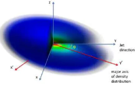
are the coordinate along the axes of the ellipsoidal distri-bution and θ is the angle between the jet and the major axis of the atmosphere. A sketch of this setup is shown in Fig. 1. In all the simulations we used ax = 1/3, ay = 2/3
and az = 1/4. The pressure distribution follows the
den-sity distribution and equilibrium is maintained by an ex-ternal gravitational potential. Two jets, with initial radius rj = 0.05rc, flowing in opposite directions are injected at
the center of the domain. No magnetic field is present in the initial configuration at t = 0, and a toroidal magnetic field is injected along with the jets. The injection region is a cylinder of radius rj and length 0.04rc aligned with
the y axis in which the variables are not evolved but they are kept fixed at the injection values. As shown in Fig. 2 this region is divided in three part, a central part (shown in black in the figure) in which velocity and magnetic field are zero, and two side regions (shown in red and blue in the figure) in which the jet velocities are opposite and the magnetic field is defined as
Bx= −Btr sin(φ) (7)
By= Btr cos φ (8)
in the blue region and is reversed in the red region. Here r and φ are polar coordinates in a plane normal to the y axis and the maximum field strength Bt is fixed by the value
of the jet magnetization, σ, which represents the ratio be-tween the Poynting flux and the matter energy flux, in the jets. A jet with a purely toroidal field is potentially unsta-ble to pinch and kink magnetohydrodynamic instabilities, however the effect of these instabilities starts to show up only at late times where some jet wiggling can be observed. The two jets are slightly perturbed at their base, in or-der to destroy all symmetries, the following evolution is in-dependent from the details of the perturbation. The param-eters that characterize this configuration are the jet Lorentz
Fig. 1. Sketch of the simulation setup showing a representation of the initial density distribution and the relative orientation of the jets.
Fig. 2. Sketch of the cylindrical injection region which rep-resents an internal boundary in which the variables are kept fixed to the injection values. In the black part velocity and magnetic field are kept equal to zero, in the blue and red regions velocities are opposite and from these two regions two opposite jets are injected. The blue and red arrows show the velocity directions, while the arrows on the yellow and green lines show the direction of the toroidal magnetic field.
factor γj, the density ratio ν, between the jet density and
the central density, the jet temperature and the magnetiza-tion σ, The temperature of the external medium is fixed by the jet Mach number Mj, which is 400 for all simulations.
In Table 1 we show all the parameters for the simulations that we present in this paper. In the sixth column of Table 1 we give the values of the jet energy flux defined by
Lj = πrj2ρjγj2c 3
= 2.5 × 10⁻³
πρ0rc2νγ2jc3 (9)
and computed for the representative values rc= 4kpc and
ρ0= 1cm−3, which are consistent with observational data.
The details of the injection setup have of course some influ-ence on the characteristics of jet propagation. However, we can expect limited differences on the large scale structure, also in view of the fact that the perturbations imposed at the base will quite likely cause the jet to lose memory of the details of the initial state, while propagating into the ambient medium.
The first three simulations (A, B and C) have constant energy fluxes, but different and decreasing Lorentz factors γj. Cases A, D and E have fixed Lorentz factor γj, but
de-creasing density ratio and consequently dede-creasing energy flux. We have also to notice that cases D and E have a ten time higher magnetization than case A, the Poynting flux of case D is then equal to that of case A. Finally, cases E and F differ only for the angle θ between the jet direction and the major axis of the atmosphere. In Table 1 we give, in the last two columns, for each case, the size of the compu-tational domain and the grid size. For all the simulations the grid is uniform in the central region (1 × 2 × 1) and is stretched in the outer parts in order to achieve larger distances. The simulations have been performed with the PLUTO code (Mignone et al. 2007), with a second order accurate linear reconstruction and HLL Riemann solver.
3. Results
In the presentation of the results, all quantities are ex-pressed in physical units, their dimensional values depend however on the choice of our unit of length rc and density
ρ0, which we have assumed rc = 4kpc and ρ0= 1cm−3. A
different choice for these units will give different values for all the relevant physical quantities, more precisely lengths scale as rc, times scale also as rc, pressure scales as ρ0 and
magnetic field strength scales as √ρ0.
In the first three simulations (A, B and C) we kept a constant jet power of 1.6 × 1046 erg s−1, but we varied
the Lorentz factor and the jet density, keeping γ2 jρj, and
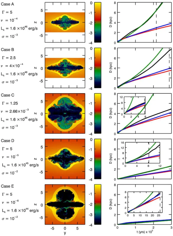
Case θ γj ν σ Lj Domain Grid A 0 5 1 × 10⁻⁴ 10−3 1.6 × 1046 2 × 4 × 2 384 × 768 × 384 B 0 2.5 4 × 10⁻⁴ 10−3 1.6 × 1046 2 × 4 × 2 384 × 768 × 384 C 0 1.25 2.66 × 10⁻³ 10−3 1.6 × 1046 4 × 4 × 4 768 × 768 × 768 D 0 5 1 × 10⁻⁵ 10−2 1.6 × 1045 4 × 8 × 4 768 × 1024 × 768 E 0 5 1 × 10⁻⁶ 10−2 1.6 × 1044 4 × 8 × 4 768 × 1024 × 768 F 30o 5 1 × 10⁻⁶ 10−2 1.6 × 1044 4 × 8 × 4 768 × 1024 × 768
Table 1.Parameters used in the simulation models. In the first column we have the case identifier, in the second column the angle between the jet axis and the major axis of the triaxial density distribution, in the third column the jet Lorentz factor, in the fourth column the density ratio, in the fifth column the magnetization parameter σ, in the sixth column the jet power, in the seventh column the size of the computational domain in units of rc and in the eighth column the
grid size.
Lj is measured in erg s−1and is computed for rc= 4 kpc and ρ0= 1 cm−3, the dependence of Lj on rc and ρ0 is given
by Eq. 9
hence the energy flux, constant. In all cases, at the injection point, the jet results to be overpressured with respect to the ambient medium, with increasing pressure going form case A to case C. In cases D and E, instead, we kept a constant Lorentz factor but we decreased the jet density and therefore the jet power which results to be 1.6 × 1045
erg s−1
in case D and 1.6 × 1044 erg s−1in case E.
In Fig. 3, the panels in the central column show, for cases A to E, 2D cuts in the yz plane of the logarithmic density distribution at the time when the jets have reached a length of approximately 8 kpc. We recall that the z di-rection corresponds to the minor axis of the triaxial distri-bution. The figures give a first impression of the relative importance of lateral wings in the different cases. The for-mation of a winged structure depends on the lateral ex-pansion velocity of the cocoon relative to the propagation velocity of the jet head. A theoretical estimate of the latter can be derived by equating the momentum flux of the jet and of the ambient medium in the frame of reference of the jet head. In the relativistic case one can derive the following expression (Mart´ı et al. 1997):
vh= γj√η 1 + γj√η vj, (10) where η = ρjhj ρaha (11) and ρj, ρa, hj, ha are respectively the jet and ambient
den-sities and the jet and ambient specific enthalpies. The am-bient density decreases as the jet propagates outward ac-cording to Eq. (4) and, acac-cording to Eq. (10), the jet head should accelerate. In the right column of Fig. 3, we can compare the actual jet head position as a function of time, represented by the black curves, with the theoretical esti-mates given by Eq. (10), represented by the green curves. In the same figures we also show the size reached by the cocoon as a function of time, in the two transverse direc-tion, the size along the z direction is represented in blue, while the size along the x direction is represented in red. Considering cases A, B and C, the initial predicted jet head velocities are the same, since γ2
jρj is kept constant, and
equal to about 2.1 × 109 cm s−1. The actual values are in
very good agreement with this estimate. These three cases, according to Eq. (10) should behave in the same way, how-ever, in reality, they show marked differences. In case A the
jet head accelerates reaching a velocity of about 4.3 × 10⁹
cm s−1
when the jet extends up to 8 kpc. The agreement between the actual and estimated velocities is very good. In case B we still observe acceleration and the velocity at 8 kpc is about 3.15 × 109 cm s−1, the comparison with the
theo-retical estimate shows an actual lower velocity, in fact the estimated velocity at 8 kpc should be as before 4.3×109cm
s−1. This effect is much more pronounced in case C, where,
instead of accelerating, the jet head decelerates, reaching a velocity of about 8.7 × 108 cm s−1 at 8 kpc. According to
Eq. (10), the jet head velocity, in our conditions, scales as √
ν and therefore the initial values reduce to 6.7 × 108cm
s−1
in case D and to 2.1 × 10⁸
cm s−1
in case E. In case D, we still observe an acceleration of the jet head, with, how-ever, a velocity lower than expected (compare the black and green curves), with an actual value of about 1.6 × 109 cm
s−1. In case E the deviation from the theoretical estimate
is more evident and the acceleration barely visible (com-pare the black and green curves), in fact the velocity at 8 kpc is only 3.13 × 10⁸
cm s−1
. Clearly the jet reaches a size of 8 kpc at progressively later times in cases D and E. The discrepancy between the actual and estimated veloc-ity can be understood by considering that, in deriving Eq. (10), it is implicit the assumption that the two areas used for balancing the momentum fluxes are equal (Lind et al. 1989; Massaglia et al. 1996), in reality the area on which the jet deposits its momentum can increase leading to a velocity lower than expected from Eq. (10). The increase in the area can occur either because of an expansion of the working surface, particularly evident in case C, or be-cause of instabilities that can fragment or induce wiggling of the jet head. In Figure 4 we compare the structures of the jet head for case A, in which the actual head veloc-ity perfectly agrees with the theoretical estimate, and for case E, in which the actual head velocity is well below the theoretical estimate. The top panels refer to case A, while the bottom panels refer to case E, left panels show a cut of the pressure distributions in the plane yz, i.e. the plane defined by the major and minor axes, while right panels show a cut of the longitudinal velocity distributions in the same plane. We can see that while in case A all the jet thrust is concentrated on a section which is comparable to the jet width, in case E the jet close to the head appears to have widened and the thrust is distributed on a larger area. This is consistent with the discussion made above and the
effect appear to become more pronounced as we decrease the density ratio.
Concerning the wing expansion, their velocity can be estimated as (Begelman & Cioffi 1989):
vw=
rp
c
ρa
(12) where pc is the average cocoon pressure, whose evolution
as a function of the jet length is represented in Fig. 5, for all cases. We see that the cocoon pressure decreases as the system evolves and its size increases. The wings expansion velocity which depends on the ratio between pcand ρa, will
increase or decrease depending on which between pressure and density decreases faster. Our results displayed in the right column of Fig. 3 show that the lateral expansion ve-locities for all cases remain approximately constant in time (blue and red curves), the decrease in the cocoon pressure is then almost balanced by the decrease in the external density.
In cases A, B and C, the cocoon pressure has approx-imately the same value and in fact the lateral expansion velocities are almost the same for all these cases, approxi-mately 109cm s−1, with the velocity along the x direction
about 10% lower than the velocity along the z direction. Notice then that the higher wing prominence in case C is due to a lower jet head velocity and not to a higher lat-eral velocity. The results for cases A, B and C show that for getting a winged source at high power the jets have to be subrelativistic. For relativistic jets we can get X-shape morphology only decreasing their power.
The decrease of the jet power leads to a decrease of the cocoon pressure, as shown in Fig. 5, and therefore to a slowing down of the wing expansion. The lateral veloci-ties reduce to about 5 × 108cm s−1in case D and to about
2.5 ×108cm s−1in case E. However, as seen above, also the
jet head velocity reduces with the jet power and the wing prominence depends on which reduces faster. In Fig. 6 we compare, for cases A, D and E, the average expansion veloc-ities along the three axes as a function of jet power. Circles represent the jet head velocity, while diamonds and squares represent the lateral expansion velocities respectively along the z and x directions. The figure shows that the jet head velocity decreases with jet power faster than the lateral ve-locities and moreover the expansion velocity along the mi-nor axis z decreases slower than the corresponding velocity along the intermediate x axis. Therefore, in conclusion, only low power relativistic jets can give origin to X-shaped mor-phologies, while high power jets have to be subrelativistic, as shown by cases A, B and C discussed above. Based on the comparison between the velocities along the z and x axes, shown in Fig 6, we expect that, increasing the ellip-ticity, the decrease of the lateral expansion velocity along the minor axis will be lower and the critical power, under which a winged morphology can be obtained, will depend on the ellipticity of the gas distribution, with a higher crit-ical power for higher ellipticity.
3.1. Case F: The effects of misalignment between jet and major axis
In this subsection we will describe the evolution of Case F, which has the same parameters as case E, but has a mis-alignment of 30obetween the jet axis and the major axis of
the density distribution and which we followed for a some-what longer time, until it reached a jet length of about 12 kpc at t ∼ 3.6 × 10⁶yrs. The most favourable condition for
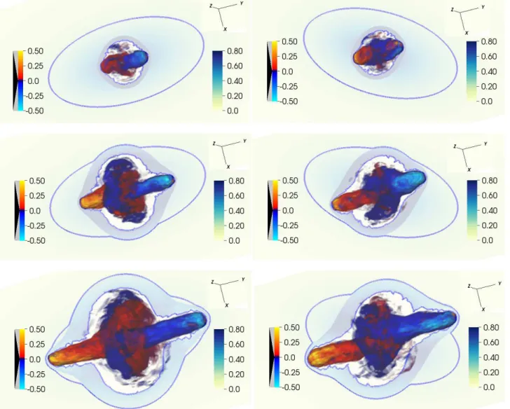
the formation of the wings is when the jet is aligned with the major axis of the galaxy, with case F we want then explore whether the X-shape morphology can develop also in a less favourable condition. Fig. 7 compares the evolution of case E and case F by showing three-dimensional volume render-ings of the distribution of the y component of the velocity, with blue colors representing negative values and red-yellow colors representing positive values. The renderings show in particular the structure of the backflows, i.e. of the jet ma-terial that after crossing the jet terminal shock flows back towards the jet origin. Superimposed, we also show a cut of the density distribution in the x − y plane, while the blue lines are density iso-contours at ρ = 0.2cm−3
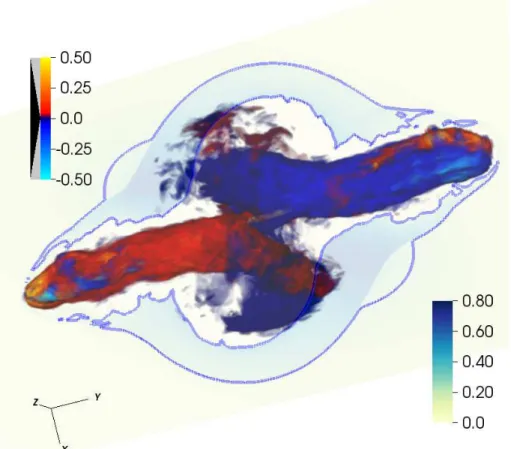
on the same plane. The density distributions and the iso-contour lines allow to follow how the initial ellipsoidal density structure is progressively modified by the inflating cocoon. The pan-els on the left are for case E, while the panpan-els on the right are for case F. The three panels on each column are for three different times showing the cocoon evolution. Finally in Fig. 8 we show only the structure of case F at a later time, for which we don’t have the corresponding image for case E, since, for this case we stopped the simulation at an earlier time. The figure shows how the cocoon progressively inflates expanding in the direction of the minor axis of the density distribution, which in case F is not perpendicular to the jet axis. As shown in the figure, the times at which case F reaches the same length as case E are somewhat ear-lier, indicating a slightly larger jet head velocity. In fact the average velocity for case F is 3.26 × 10⁸
cm s−1
to be com-pared to 2.8 ×108cm s−1. The lateral expansion velocity is,
on the contrary, slightly lower in case F than in case E. The initial density distribution, that at the beginning strongly influences the cocoon evolution, is completely modified by the jet propagation, which inflates a cavity and forms a compressed shell at the border of the cavity. In addition we can follow the interaction of the two backflows, with one of them always prevailing on the other and breaking, in case E, the initial symmetry. In case F the jets form non sym-metric backflows that bend towards the minor axis of the initial density distribution flowing up in the wings, as it can be seen in Fig. 8. In case F the wing axis form an angle of about 70◦
with the initial jet axis, almost constant with time, and slightly larger than the angle of 60◦
formed by the jet axis with the minor axis of the density distribution. Fig. 9 shows the distribution of pressure in the two planes (xy) and (yz), when the radio source has reached the maximal size at t ∼ 3.2 × 10⁶ yrs, with superimposed
the velocity field. The red ellipses represent an equicon-tour of the initial density distribution. In the two panels we show respectively cuts in the x − y plane (left panel) and in the y − z plane (right panel). The two panels allow to observe the effect of the misalignment on the final geo-metrical structure, already evident in Fig. 7. In addition we can see that the cocoon is still strongly overpressured with respect to the ambient. Looking at the velocity field, whose streamlines are visible in the same figure, we can observe the presence of flows rising in the wings.
The conclusion of the analysis of case F is that the prominence of wings is lower than in case E, as could be expected, since the jet direction has been moved away from the most favourable condition of perfect alignment with the
Fig. 3.The panels in the central column show 2D cuts of the logarithmic density distributions in the yz plane for cases A to E, at the time when the cocoon has reached a size of approximately 8 kpc in the y direction (the times of each snapshot is shown in the right panels by the vertical dashed lines). The density is in units of ρ0. The right panels show plots of
the cocoon size along the three axes (black along y, blue along z and red along x) as a function of time up to 3 × 10⁵
yrs, we recall that the z direction corresponds to the minor axis, while the x direction corresponds to the intermediate axis. The green lines show the theoretical estimate of the jet head position based on Eq. 10 Since the expansion of cases C, D and E is slower, the insets in the three bottom figures show the evolution for later times. The parameters for each case are given on the left.
Fig. 4.The left panels show the pressure distributions in the yz plane, i.e. the plane defined by the major and minor axes, while the right panels show the velocity distributions in the same plane, respectively for cases A (top) and E (bottom). The pressure is in units of ρ0c2, while the velocity is in units of c. We show only a part of the right jet in order to display
the structure of the jet head.
Fig. 5.Plot of the average pressure (averaged over the co-coon volume) as a function of jet length for all cases.
major axis of the initial density distribution. This inclina-tion of 30o, however, is still favourable for the formation of
a winged source.
Summarizing, we showed that jets with a power larger than 1045
erg s−1
have to be non relativistic in order to form a winged structure, while relativistic jets can form a winged structure only if they have Lj .1044erg s−1. Bˆırzan et al.
(2004) estimated the jet power from the observations of the X-ray cavities inflated by radio AGN. The ratio between Lj
and the radio power at 1.4 GHz (P1.4) ranges from ∼ 3 to
∼ 300 and this leads to an estimate of P1.4.3 × 1043erg
s−1
for the maximum radio luminosity of winged sources; this value compares favourably with the power distribution of X-shaped radio sources, that reaches P1.4∼ 2 × 1043erg
s−1 (Gillone et al. 2016).
3.2. Magnetic field structure
An important question to be analysed is whether the flows rising in the wings are able to carry the magnetic field
nec-Fig. 6.Expansion velocities along the three axes as a func-tion of the jet power. Circles are for the y direcfunc-tion, dia-monds for the z direction and squares for the x direction.
essary for sustaining the synchrotron radiation. In order to answer this question, we first examine in Fig. 10 the dis-tribution of the magnetic field strength, for case E at time t = 2.6 × 10⁶
yrs, in the xy and yz planes, correspond-ing, respectively, to the planes of the major and minor axes (xy, left panel) and of the major and intermediate axes (yz, right panel). The field strength is expressed in micro-gauss and is computed by assuming for the basic physical units rcand ρ0their reference values, recalling that the field
strength scales as ρ1/20 . From the figure we see that the field
strength in the jets reaches maximum values between 30µG and 60µG, similar values can be also found in the wings in the xy plane and in the lower part of the wings in the yz plane, while the upper part of the wings in the yz plane
Fig. 7. Evolution of cases E and F. The three panels on the left are for case E at times respectively 9.6 × 10⁵ yrs,
1.8 × 10⁶
yrs, and 2.6 × 10⁶
yrs,, from top to bottom, while the three panels on the right are for case F at times respectively 9.6 × 10⁵
yrs, 1.6 × 10⁶
yrs, , 2.3 × 10⁶ yrs, from top to bottom. The distribution of y velocity component
is represented by a volume rendering, with blue colors representing negative values and red-yellow colors representing positive values. Superimposed, we also show a cut of the density distribution in the x − y plane, while the blue lines are density iso-contours at ρ = 0.2cm−3 on the same plane.
shows lower values. One question that immediately arises is whether the magnetic field becomes dynamically impor-tant, we have then examined the distribution of the local values of the plasma β representing the ratio between ther-mal and magnetic pressure and we have seen that there are only a few points where it reaches values of the or-der of unity, while for the most part it has values much larger than unity and therefore it is generally dynamically unimportant. A more quantitative comparison between the magnetic field strength in the jets and in the wings is pro-vided by Fig. 11 where we plot the distribution functions of the magnetic field strength in the jet and in the wings. The jet is defined as a cylinder of radius 0.3rc with its axis
aligned with the y axis, while the wings are defined as the region external to this cylinder. From the figure we see that the maximum of the distribution is about 15µG in the jets and about 5µG in the wings, the medians of the distribu-tions are however much closer, since they are again 15µG in the jets, but about 10µG in the wings. This means that
half of the volume in the jets has field strength larger than 15µG, while in the wings, in order to get half of the vol-ume, we have to lower the threshold to 10µG. Regions with field strength larger than 30µG have very small filling fac-tors, of about 7% in the jets and 1.5% in the wings. The distribution of magnetic field described above represents a snapshot of the evolution at t = 2.6 × 10⁶ yrs, at the
end of the simulations, if we look at the complete tempo-ral evolution, we can see that the spatial distribution and the distribution function of the field strength do not change much in time, however the average field strength decreases with time as represented in Fig. 12. The value of the field depends of course on the value of σ, representing the ratio of the Poynting flux to the matter energy flux, in this case σ = 10−2. Note that the values of the resulting field
ampli-tude are quite consistent with observations. Increasing σ we expect that the magnetic field scale as √σ until it reaches values for which it becomes dynamically important. The regime in which the magnetic field becomes dynamically
Fig. 8.Backflow structure for case F at t = 3.2 × 10⁶ yrs. The representation is the same as in Fig. 7
Fig. 9. 2D cuts of the pressure distribution in the yx (on the left) and yz (on the right) planes for case F, at the time when the cocoon has reached a size of approximately 24 kpc in the y direction. Superimposed we show also the velocity field. The red ellipses represents equicontours of the initial density distribution and indicate the relative orientation of the jet with respect to the density distribution.
important is not examined in this paper, however it could be of interest for further investigations.
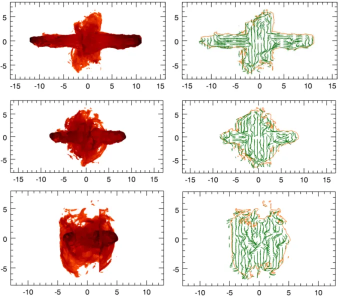
3.3. Synthetic radiomaps
In Fig. 13 we display synthetic surface brightness and polar-ization maps for different viewing angles. The calculations of the surface brightness and of the polarization are de-scribed in the appendix A. In the left panels we show the brightness maps, while in the right panels we show the po-larization maps, plotting the magnetic field direction. The line of sight is in the xy plane and from top to bottom makes with the jet direction angles respectively of 90◦
, 45◦
and 20◦
. Decreasing the viewing angle, the size of the wings
becomes more prominent as the projected jet length de-creases, until, at the smallest viewing angles, the main lobes are projected onto the wings.
We can compare the synthetic maps of the surface brightness distribution in Fig. 13 with radio maps of X-shaped sources. The synthetic map in the top-left panel of Fig. 12, viewing angle of 90◦
is reminiscent, for instance, of the radio map 3C 136.1 (Fig. 14, left panel, from Lal & Rao 2007). Considering the middle-left panel of Fig. 12, view-ing angle of 45◦
, the synthetic map can be compared to the morphology displayed by the source J1434+5906 (from Roberts et al. 2015) and shown in Fig. 14 (middle panel). The bottom-left panel of Fig. 12, viewing angle of 20◦
, compares nicely with the source J1043+3131 (again from
Fig. 10.Two-dimensional cuts of the distribution of the magnetic field strength. The left panel is in the xy plane, the right panel is in the yz plane. The field strength is expressed in microGauss, assuming for the basic physical units rc and
ρ0 their reference values.
Fig. 11. Distribution functions of the magnetic field strength in the jet (black curve) and in the wings (red curve). The dashed lines indicate the medians of the distri-butions.
Roberts et al. (2015)) and shown in Fig. 14 (right panel). Within our model, the variety of morphologies displayed by X-shaped sources can the be interpreted, beside the general effects of the the main physical parameters, by the combi-nation of different viewing angles and the orientation of the jet direction with respect to the major axis of the host galaxy. In particular, sources with a morphology similar to J1043+3131 are not usually classified as classical X-shaped, however our 3D results show that X-shaped sources can in-deed take this morphology if the line of sight form a small angle with the jet direction.
From our polarization maps we see that the magnetic field is directed along the jets and along the wings, becom-ing transverse only at the edges. This kind of morphology can be observed also in actual sources, as we can see in Fig. 15, where we show the polarization map of 3C 223.1 (from Dennett-Thorpe et al. (2002), left panel) and the one of 3C 136.1 (from Rottmann (2001), right panel). These maps have to be compared with the right panels of Fig. 13.
The emission here is treated in a simplified way and, since we do not model the evolution of the emitting non-thermal particles, we have to give a prescription for the their density and distribution. Different prescriptions may
Fig. 12.Plot of the average magnetic field as a function of time for case E.
lead to some differences in the synthetic maps. We have then considered an alternative in which we prescribe local equipartition between the magnetic energy and the energy of non-thermal particles. In Fig. 16 we show, for this choice, the synthetic map of the surface brightness distribution for line of sight at 90◦
with the jet direction, corresponding to the top left panel in Fig.13. Comparing the two maps, we can observe an overall similarity, the main differences are in the jets and in the central part of the wings which show a somewhat higher brightness.
A final remark concerns the distribution of the offset between the host major axis and the wings. Capetti et al. (2002) and Gillone et al. (2016) found that in only one source (out of 31) the wings form an angle smaller than 40o and this is the key observing result that motivated the
simulations presented in this paper. However, this finding carries further information on the wings structure. In fact, in case the wings were linear and essentially one dimen-sional features, a significant fraction of X-shaped sources should show, due to projection effects, small misalignments; this would occur when the plane defined by the wings axis and the major axis of the host forms a large angle with the plane of the sky. Our simulations show instead that the wings form a flattened emitting region aligned with a plane
including the host minor axis; the projection of such essen-tially two-dimensional structure leads to a narrower range of offsets, as observed.
4. Summary
We presented 3D relativistic magnetohydrodynamic simu-lations of bidirectional jets propagating in a triaxial den-sity distribution in order to investigate the mechanism of formation of X-shaped radiogalaxies. In Paper I we pro-posed a hydrodynamic mechanism for the formation of this class of sources and we performed 2D simulations of the propagation of a jet in an ellipsoidal density distribution. We showed that, when the jet propagates along the major axis of the distribution a winged structure can form. Here we extended our previous results, relaxing the axial sym-metry, introducing magnetic field and relativistic effects. We investigated, in particular, under which conditions of jet power, Lorentz gamma factor, and density ratio, an X-shaped structure arises. We showed that jets with a power larger than 1045
erg s−1
have to be non relativistic in order to form a winged structure, while relativistic jets can form a winged structure only if they have Lj.1044 erg s−1. By
applying a scaling relation between jet and radio power, we estimated that the maximum radio luminosity of a winged source is ∼ 3 × 1043 erg s−1, a value compatible with the
observations of X-shaped radio sources. Moreover we con-sidered a case in which the jet is misaligned with respect to the major axis of the density distribution and showed that an angle of 30o is still favourable to the formation of
an X-shaped structure.
Hodges-Kluck & Reynolds (2011) also performed three-dimensional simulations for a configuration similar to ours, they did not include magnetic field and relativistic effects. An important difference between their analysis and ours is the range of spatial and temporal scales considered. We focus on the first phases of the evolution limiting to time scales of the order of 106yrs and spatial scales of the order
of 10 kpc, when the jet still propagates within the galac-tic atmospheres, while they consider the full life of the ra-diosource and study its evolution when the jet is switched-off, the spatial scales are also larger, and the jet propagates in the cluster environment. In this sense the two approaches can be considered as complementary: the first phases of the evolution, that we consider, are essential for the forma-tion of an X-shaped radiosource and the condiforma-tions that we find are necessary conditions, while the results obtained by Hodges-Kluck & Reynolds (2011) give important insights on the subsequent long term evolution.
We have also calculated the brightness distribution producing synthetic emission maps. Being the simulated sources intrinsically three-dimensional, i.e. displaying a tri-axial structure, the same objects may appear differently as seen from varying viewing angles. We show that differ-ent observed morphologies of X-shaped sources can be the result of similar structures viewed under different perspec-tives. By considering both the structure of the wings and the triaxiality of their hosts, the relative orientation of ra-dio and optical structures has a complex dependence on the projection; this leads not only to favour large offsets between the wings and the host major axis, but also to the observed paucity of offset smaller than ∼ 40o.
Finally we remark that we carried out a simplified treat-ment of the emission. In reality, one should consider the
evolution of a distribution of relativistic electrons, carried along the jets and streaming in the wings, that lose en-ergy via synchrotron losses and adiabatic expansion, and gain energy by shock acceleration and/or via turbulent ac-celeration by IInd order stochastic Fermi-like process (see Vaidya et al. 2017 to be submitted). Our results show that shocks in the wings are quite weak and therefore they will most likely contribute in a limited way to particle reaccel-eration, however reacceleration by turbulence may be more effective. Further studies are then required to examine the behavior of the spectral index in the wing, compared to observations.
Acknowledgments
We acknowledge the CINECA award under the ISCRA ini-tiative, for the availability of high performance computing resources and support. This work has been partly funded by a PRIN-INAF 2014 grant.
References
Begelman, M. C. & Cioffi, D. F. 1989, ApJ, 345, L21
Bˆırzan, L., Rafferty, D. A., McNamara, B. R., Wise, M. W., & Nulsen, P. E. J. 2004, ApJ, 607, 800
Capetti, A., Zamfir, S., Rossi, P., et al. 2002, A&A, 394, 39 Cavaliere, A. & Fusco-Femiano, R. 1976, A&A, 49, 137 Cheung, C. C. 2007, AJ, 133, 2097
Del Zanna, L., Volpi, D., Amato, E., & Bucciantini, N. 2006, A&A, 453, 621
Dennett-Thorpe, J., Scheuer, P. A. G., Laing, R. A., et al. 2002, MNRAS, 330, 609
Ekers, R. D., Fanti, R., Lari, C., & Parma, P. 1978, Nature, 276, 588 Fanaroff, B. L. & Riley, J. M. 1974, MNRAS, 167, 31P
Gillone, M., Capetti, A., & Rossi, P. 2016, A&A, 587, A25
Gopal-Krishna, Biermann, P. L., Gergely, L., & Wiita, P. J. 2012, Research in Astronomy and Astrophysics, 12, 127
Hodges-Kluck, E. J. & Reynolds, C. S. 2011, ApJ, 733, 58
Klein, U., Mack, K.-H., Gregorini, L., & Parma, P. 1995, A&A, 303, 427
Lal, D. V. & Rao, A. P. 2007, MNRAS, 374, 1085 Leahy, J. P. & Williams, A. G. 1984, MNRAS, 210, 929
Lind, K. R., Payne, D. G., Meier, D. L., & Blandford, R. D. 1989, ApJ, 344, 89
Mart´ı, J. M., M¨uller, E., Font, J. A., Ib´a˜nez, J. M. Z., & Marquina, A. 1997, ApJ, 479, 151
Massaglia, S., Bodo, G., & Ferrari, A. 1996, A&A, 307, 997 Mignone, A., Bodo, G., Massaglia, S., et al. 2007, ApJS, 170, 228 Mignone, A., Plewa, T., & Bodo, G. 2005, ApJS, 160, 199 Rees, M. J. 1978, Nature, 275, 516
Roberts, D. H., Cohen, J. P., Lu, J., Saripalli, L., & Subrahmanyan, R. 2015, ApJS, 220, 7
Rottmann, H. 2001, PhD thesis, Thesis (Ph.D.) – University Bonn, 2001, 180 pages
Vaidya, B., Mignone, A., Bodo, G., Rossi, P., & Massaglia, S. 2017 to be submitted
Wirth, A., Smarr, L., & Gallagher, J. S. 1982, AJ, 87, 602
Worrall, D. M., Birkinshaw, M., & Cameron, R. A. 1995, ApJ, 449, 93
Appendix A: Surface brightness and polarization
maps
The surface brightness radio maps and polarization maps have been obtained by integrating along the line of sight respectively the synchrotron emissivity j and the Stokes parameters Q and U . The synchrotron emissivity in the comoving frame, for a power law distribution of relativistic
Fig. 13.Synthetic radio surface brightness and polarization maps for different line of sights, for case F. The panels on the left show the brightness maps, with the line of sight in the xy plane, while those on the right show the polarization maps (the magnetic field direction is plotted). For the top panels the line of sight makes an angle of 90◦
with the jet direction, in the middle the angle is 45◦
and at the bottom the angle is 20◦
. The brightness maps have a logarithmic scaling and cover a range of four order of magnitude.
Fig. 14. 610 MHz radio map of the source 3C 136.1 observed at GMRT (Lal & Rao 2007) (left panel); 1.4 GHz radio map of the source J1434+5906 observed at VLA (Roberts et al. 2015) (middle panel); 1.4 GHz radio map of the source J1043+3131 observed at VLA (Roberts et al. 2015) (right panel)
electrons is (Del Zanna et al. 2006) j′
(ν′
) = K|B′
× n′
|α+1ν′−α (A.1)
where all primed quantities are computed in the proper frame, n′
represents the versor corresponding to the line of
sight direction, K is a constant proportional to the number density of relativistic electrons and −(2α + 1) is the slope of the energy distribution of relativistic particles. In order to obtain the emissivity in the observer frame, we have to
Fig. 15.Polarization maps of the source 3C 223.1 (Dennett-Thorpe et al. 2002) (left panel) and of 3C 136.1 (Rottmann (2001)) (right panel)
Fig. 16. Synthetic radio surface brightness map, for case F, computed assuming local equipartition between the magnetic energy and the energy in non-thermal particles. The line of sight makes an angle of 90◦
with the jet direction and the map corresponds to the top left panel in Fig. 13. The brightness map, as in Fig. 13 has a logarithmic scaling and cover a range of four order of magnitude.
take into account relativistic corrections and we get j(ν) = K|B′
× n′
|α+1Dα+2ν−α (A.2)
where D is the Doppler factor
D = 1
γ(1 − β · n) (A.3)
Considering a cartesian reference frame in which X is along the line of sight and Y and Z are in the plane of the sky,
the surface brightness can be obtained as I(ν, Y, Z) =
Z ∞ −∞
j(ν, X, Y, Z)dX (A.4) and the Stokes parameters Q and U are given by
Q(ν, Y, Z) = α + 1 α + 5/3
Z ∞ −∞
U (ν, Y, Z) = α + 1 α + 5/3
Z ∞ −∞
j(ν, X, Y, Z) sin 2χdX (A.6) where χ is the local polarization position angle, measured clockwise from the Z axis. From Q and U we can then get the observed polarization direction. In our calculations we assumed the density of relativistic electrons to be pro-portional to the local fluid density and the spectral index α = 0.5.