DOI 10.1007/s12567-015-0081-5
ORIGINAL PAPER
ESA multibody simulator for spacecrafts’ ascent and landing
in a microgravity environment
Mario Toso · Ettore Pennestrì · Valerio Rossi
Received: 31 October 2014 / Revised: 16 January 2015 / Accepted: 9 February 2015 © CEAS 2015
CoG Centre of gravity
DCAP Dynamic and control analysis package
DOF Degree(s) of freedom
EOM Equations of motion
ESA European Space Agency
ESTEC European Space Research and Technology
Centre
EXOMARS Exobiology on Mars mission
GNC Guidance, navigation and control
JAXA Japan Aerospace Exploration Agency
JPL Jet propulsion laboratory
NASA National Aeronautics and Space
Administration
ODE Ordinary differential equation
PECE Prediction-evaluation-correction-evaluation method
S/C Spacecraft
TEC-MSM ESA’s mechanisms section
1 Introduction
Exploring the diverse objects in our Solar System is the heart of space agencies scientific objectives, from the early manned exploration of the moon in the 60s to the most recent robotic missions to asteroids, comets and planets [1–3].
Few examples can effectively illustrate the diverse challenges of exploration missions: JAXA Hayabusa mis-sion [4, 5] attempted to take samples from the surface of the asteroid Itokawa and successfully returned it to Earth in 2010; ESAs cornerstone mission Rosetta [6] has been the first to rendezvous with a comet and to deploy a lander (Philae) on the comets nucleus in 2014. In the last decade, NASA has successfully landed on Mars multiple rovers [7]
Abstract The investigation of planets, moons and small
bodies, including comets and asteroids can contribute sub-stantially to our understanding of the formation and history of the solar system. In situ observations by landers play an important role in this field: for example, the Rosetta Lander Philae has been the first spacecraft to accomplish a soft touchdown on a comet. Since the last decade, the urgency to anticipate hardware performance and correlate testing results with mathematical models is generating the trend for more extensively applying multibody approach in sup-porting the design and verification of complex aerospace systems, from the early phases of the project. Some of the essential multibody technologies assisting the analysis of this class of problems consist of a reliable attitude control algorithm, a variable-step and variable-order numerical integrator and a consistent contact-friction formulation. This paper illustrates the particular implementation of these crucial features in the European Space Agency’s multibody software DCAP and shows a direct application to a feasi-bility case study.
Keywords Multibody · DCAP · Landing · Touchdown ·
Quaternions · Integrator · Contact · Sloshing
Abbreviations
CDF Concurrent design facility
M. Toso
ATG ESA/ESTEC, Keplerlaan 1, 2201AZ Noordwijk ZH, The Netherlands
e-mail: [email protected] E. Pennestrì · V. Rossi (*)
Università degli Studi di Roma Tor Vergata, Via del Politecnico 1, Rome, Italy
(Curiosity landed in 2012), ESA is adding to this list the EXOMARS missions [8] with Russian partnership and also China and India are planning exploration missions to the Earth’s moon and the red planet before 2020. Moreover, the CleanSpace program [9] and other Earth low orbit debris removal missions such as e.Deorbit [10], currently in phase A, heavily rely on multibody simulations for both the com-plex close proximity capture operation and for analysis of the elastic dynamics during the de-orbiting burn.
Building on the 50 years heritage of the European Space Agency’s Technology Center in providing effective spacecraft design and simulations technical solutions, this paper addresses the latest improvements implemented in the ESA multibody software DCAP, especially dedicated to ease simulating system dynamics during the landing of a spacecraft, in the frame of a feasibility study (CDF) and preliminary design verification activities. This paper builds on DCAP release 8.0, which includes extending the usa-bility of the complementary features already discussed in recent papers by G. Baldesi et al. (e.g. launcher lift-off and multi-stage separation [11], integrated ascent and guidance approach [12]).
For the purpose of simulating a realistic descent and landing of a spacecraft, the complexity of three-dimen-sional motion has to be supported by a robust orientation algorithm capable of always describing the attitude of the body. In Sect. 2 of this paper, the Euler angles implemented in DCAP release 8.0 have been substituted with quaterni-ons, to avoid numerical singularities for particular space-craft orientations.
Touchdown technologies aim at providing effective solutions to unpredictable and/or occasional fast dynamics discontinuous events. Fixed-time step 4th order Runge– Kutta integrator, which is the one implemented in DCAP release 8.0, is intrinsically limited in accurately simulating these type of events; as for other tools based on fixed-step integrators, the provision of an elaborate time reset and step-back subroutines logic has been able to partially com-pensate for the lack of automatic event detection and step adaptation in the DCAP package. Alternatively and more effectively, in the authors opinion, sudden discrete events can be comprehensively tackled by numerical integrators with variable time step and algorithm order, capable of effectively recognizing the discontinuity and automatically tune the solver parameters to match the overall required tolerance. Moreover, this family of integrators is known to exhibit outstanding computational speed. In the DCAP implementation proposed in Sect. 3, the additional advan-tage is to eliminate the need for the complicated time-reset and step-back interconnected logic management by directly delegating its function to the integrator itself. This enables to further increase the overall computational speed and accuracy, to automatically detect discrete events and to
simplify the tree of dependencies and management of the exceptions cases which, in return, also decreases the risk of incorrect outputs.
Adequate representation of the soil dynamic proper-ties [13–15] as well as the lander structure [16] and shock absorbing characteristics [17] are key parameters for deter-mining the equivalent friction between the lander and the soil. Also, a proper selection of a number of parameters [18] such as the vertical and lateral landing velocities and the spacecraft inclination angle of the landing target can determine the margin of risk to crash, bounce or tip over during landing. Considering the general objective of main-taining a synthetic and versatile approach, after reviewing more enhanced three-dimensional contact representations [19, 20] and their implementation in state-of-the-art com-mercial software packages, a trade-off between complex parameter management versus global effectiveness goes in favor of a simpler consolidated model. A straightforward contact formulation based on Hertz theory is therefore pre-sented in Sect. 4.
An example of landing simulation is then presented in the Sect. 5. The adopted approach is typical of feasibility studies, such as those performed in the European Space Agency’s Concurrent Design Facility (CDF), where a num-ber of versatile conceptual models are used in parallel to check for design feasibility and requirements consistency, as well as to rapidly simulate and compare the foresee-able mission scenarios. Moreover, the comparison with the results obtained with an independent commercial software is also shown for completeness.
Finally, conclusions are drawn in the Sect. 6.
2 Quaternions
2.1 Background on quaternions
Euler angles are widely used in multibody software to describe the attitude of bodies by representing the tion of a reference frame relative to another. Any orienta-tion can be described by a sequence of three element rota-tions. There are 12 different sequence conventions of Euler angles.
In multibody simulations, Euler angles are also used during the numerical integration. The dynamic routine of a multibody software produces the accelerations of the system and by integrating them the entire kinematics of the system is obtained. Unfortunately, by referring only to rotational degrees of freedom for simplicity, it is possible to integrate the angular accelerations into angular velocities, but it is erroneous to integrate angular velocities to obtain the attitude values, because the angular velocity is not an exact differential [21]. Therefore, the equations of motion
are generally formulated in terms of Euler angles and their derivatives, because it is allowed to double integrate the double dot Euler angles { ¨θ} to obtain the Euler angles. The following relations convert Euler angles derivatives into angular velocities and accelerations:
where the vectors {ω} and { ˙ω} contain the angular velocities and accelerations of a generic body, the vector { ˙θ} and { ¨θ} contain the first and second Euler angles derivatives and the matrix [L] and [ ˙L] are used for the conversion.
The main disadvantage of using the Euler angles is the numerical phenomenon of gimbal lock. In particular sys-tem configurations, the matrix [L] becomes singular and the inverse relation can no more be extracted.
For example, assuming to use the Euler angles conven-tion 1-2-3, the relaconven-tion becomes:
where the matrix [L123] is defined as:
The inverse relation can been written as: where the matrix [L123]−1 is:
For this particular Euler angles convention, the condition of gimbal lock occurs at Euler angle θ2= 90◦, as the
compo-nents of matrix [L123]−1 tends to infinity.
Introducing quaternions as an alternative to Euler angles is recognized as a valuable option to avoid the gimbal lock phenomenon. In this case, the relation of the angular veloc-ity turns out to be [21]:
(1) {ω} = [L]{ ˙θ } (2) { ˙ω} = [L]{ ¨θ } + [ ˙L]{ ˙θ } (3) {ω} = [L123]{ ˙θ } (4) [L123] =
cos θ2cos θ3 sin θ3 0 − cos θ2sin θ3 cos θ3 0
sin θ2 0 1 (5) { ˙θ } = [L123]−1{ω} (6) [L123]−1= � cos θ3 cos θ2 � −�sin θ3 cos θ2 � 0 sin θ3 cos θ3 0 −�cos θ3sin θ3 cos θ2 � � sin θ3sin θ2 cos θ2 � 1
where the vector {˙p} is the first time derivative of the rela-tive quaternions and the matrix [Q] is defined as:
and pi are the four quaternions defined as:
where θ is the rotation about the screw axis ˆu. 2.2 Quaternions implementation in DCAP
The Order(n) algorithm [11], used by DCAP release 8.0 to evaluate the dynamics of the system, produces equations of motion in terms of Euler angles derivatives. The algorithm treats separately all the hinges of the system, which are the connections between bodies. In this framework, only hinges with 3 rotational degrees of freedom could poten-tially experience gimbal lock.
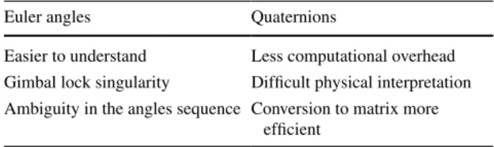
The quaternions implementation has been designed so that, although DCAP will rely on quaternions for comput-ing the kinematics of the system, Euler angles will still always be produced as standard output angles, because of their direct physical interpretation. This architecture achieves the known benefits from a computational pro-spective, see Table 1, while hiding the only main drawback which is the lack of intuitiveness from a user prospective.
The recoded internal symbolic generator has been ena-bled to assemble the equations of motion using the angular velocities {ω} and accelerations { ˙ω}, instead of { ˙θ} and { ¨θ}, as generalized coordinates.
Considering an open loop topology system, it is usual to refer to the body L(j) as the lower body of the body j, within the topology tree. Using Euler angles the following equations are used in DCAP:
where {L(j)ωj} is the relative angular velocities vector,
{L(j)ω˙j} is the relative angular accelerations vector and
{L(j) ◦ω
vj} is the remainder terms vector between the body j
and its lower body L(j).
(7) {ω} = 2[Q]{˙p} (8) = −p1 p0 p3 −p2 −p2 −p3 p0 p1 −p3 p2 −p1 p0 (9) p0= cos θ 2 p1= ux sinθ 2 p2= uy sinθ 2 p3= uzsin θ 2 (10) {L(j)ωj} = Lj { ˙θj} (11) {L(j)ω˙j} = [Lj]{ ¨θj} + L(j) ◦ωvj
Table 1 General pros and cons of Euler angles versus quaternions
Euler angles Quaternions
Easier to understand Less computational overhead Gimbal lock singularity Difficult physical interpretation Ambiguity in the angles sequence Conversion to matrix more
From this, it is possible to compute the equations of motion in the same way and using the same routine, but considering physical entities such as angular veloci-ties {L(j)ωj} and angular accelerations {L(j)ω˙j}, instead of
the Euler angles derivatives, by means of the following substitution:
where [I] is the identity matrix. In this way, the vectors
{L(j)ωj} and {L(j)ω˙j} are equal to the vectors { ˙θj} and { ¨θj} and
they can be used as generalized coordinates. This simple mathematical substitution allows the rest of the DCAP core algorithm to be unchanged and avoids the complete recon-ditioning of the equations of motion generator algorithm.
Considering only rotational DOF for simplicity, since the EOM are derived using Kane’s method of generalized speeds [22], the partial velocity matrices can be written as:
where { ˙Rj} is the linear velocity vector of the CoG of the
body j and { ˙ωj} is the angular velocity vector of the body j.
These partial velocity matrices will be automatically computed using the aforementioned substitutions (12) and (13) and no additional modifications to the EOM generator are necessary.
The state vector derivative between two bodies L(j) and j, in the original DCAP algorithm, is:
while, after the aforementioned substitution, it can be expressed as follows:
Before integrating, the state vector derivative is then trans-formed into:
where: –
– the vector {L(j)˙pj} contains the derivatives of the
quater-nions: (12) [Lj] = [I] (13) L(j) ◦ω vj = {0} (14) [Vj] = ∂{ ˙R j} ∂{L(j)ωj} (15) [ωj] = ∂{ ˙ω j} ∂{L(j)ωj} (16) {L(j)X˙j} = { L(j)θ¨j} {L(j)θ˙j} (17) {L(j)X˙j} = { L(j)ω˙j} {L(j)ωj} (18) {L(j)X˙j} = {L(j)ω˙j} 0.5[L(j)Qj]T{L(j)ωj} = { L(j)ω˙j} {L(j)˙pj} {L(j)˙pj}T = L(j)˙pj 0 L(j)˙p j 1 L(j)˙p j 2 L(j)˙p j 3 ; –
– the matrix [L(j)Qj] is used to convert quaternions into
angular velocity:
After integrating, the state vector becomes:
Each quaternion must be normalized by evaluating the norm of the vector and dividing each component by the norm:
where L(j)pˆ
ij is the normalized quaternion.
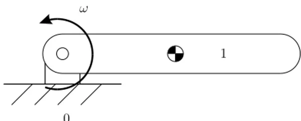
As the non-linear time simulation algorithm requires Euler angles to evaluate the transformation matrices between bodies, also the modified algorithm retrieves the Euler angles at each time step from the quaternions [23]. 2.3 Example of gimbal lock and quaternions results Figure 1 shows a simple system composed by one body linked with a spherical hinge (3 rotational DOF) to the ground. The body 1 is initially rotated of 85° around the second Euler angle axis and an initial velocity ω of 10°/s is imposed. The Euler angles sequence 1-2-3 is chosen for this example, which exhibits gimbal lock at 90°.
Two simulations are compared: one using the original DCAP with Euler angles and one using the modified DCAP with quaternions.
The results are reported in Fig. 2: as expected, when the body 1 reaches the gimbal lock configuration (θ2= 90◦)
the numerical integration based on Euler angles crashes, while the one based on quaternions seamlessly progresses through. [L(j) Qj] = −L(j) p1j L(j)p0j L(j)p3j −L(j)p2j −L(j) p2j −L(j)p3j L(j)p0j L(j)p1j −L(j) p3j L(j)p2j −L(j)p1j L(j)p0j . (19) {L(j)Xj} = { L(j)ωj} {L(j)pj} (20) L(j) ˆ p0j= L(j) p0j |{L(j)pj}| , L(j) ˆ p1j = L(j) p1j |{L(j)pj}| , L(j) ˆ p2j= L(j) p2j |{L(j)pj}| , L(j) ˆ p3j = L(j) p3j |{L(j)pj}| 0 1 ω
3 PECE integrator
The ODE solver, selected for DCAP, was developed by Shampine and Gordon [24] in collaboration with Sandia Laboratories and the University of New Mex-ico in 1974. It is based on a PECE Adams–Bashforth– Moulton algorithm with variable-step size and varia-ble-order algorithm, and the code is written in Fortran language.
3.1 Background on PECE algorithm
A PECE algorithm is a Prediction-Evaluation–Correc-tion-Evaluation method and both explicit and implicit methods are used. The sequence of actions are here summarized:
–
– Prediction an explicit Adams–Bashforth method of order k is used to predict the value yn+1;
–
– Evaluation the function fp
n+1 at tn+1 is evaluated by
means of the value yn+1;
–
– Correction an implicit Adams-Moulton method of order k +1 is then used to correct the previous value and to
obtain a more accurate estimation of the solution, yn+1;
–
– Evaluation another evaluation of the function fn+1 is
carried out.
Adams method approximates the derivative with a polyno-mial interpolating the computed derivative values and then integrates the polynomial. The variable step size is able to follow the slow or fast modifications of the function during the integration.
The Adams–Bashforth method for variable step size is:
where pn+1 stands for the predictor of the PECE algorithm
and k is the order of the method. Quantities in Eq. (21) are defined as [24]:
where hi is the time step and αi(n) and βi(n) are defined as:
and the coefficient gi,1 is identified by:
(21) pn+1= yn+ hn+1 k i=1 gi,1φ∗i(n) (22) φ∗i(n) = βi(n +1)φi(n) (23) φ1(n) = f [xn] (24) φi(n) = f [xn, xn−1, . . . , xn−i+1] i j=2 �j−1(n) i >1 (25) �i(n +1) = i j=1 hn+2−j (26) αi(n +1) = hn+1 �i(n +1) i ≥1 (27) β1(n +1) = 1 (28) βi(n +1) = i j=2�j−1(n +1) i j=2�j−1(n) i >1 (29) g1,q= 1 q Fig. 2 The evolution of the
sec-ond Euler angle in both Euler angles case and quaternions case is reported on the left, the quaternions evolution is shown on the right, for the modified DCAP simulation 0 1 2 3 4 5 80 90 100 110 120 130 140 0 1 2 3 4 5 0 0.1 0.2 0.3 0.4 0.5 0.6 0.7 0.8 0.9 1
where the parameter is an integer number q = 1, 2, 3 . . . . The Adams–Moulton method with variable step size uses the same data of the predictor method, plus an additional one, accounting for the order k + 1 of the corrector, therefore:
The main advantage of this formula is the possibility to evaluate gk+1,1 during the prediction process. In this case,
the last factor in (32) is defined as:
Since the algorithm of order k is not self-starting, it is always necessary to start from a first order method and than increase the order up to the desired one.
The ODE algorithm identifies the adequate step size able to minimize the local error, which translates into approxi-mating the local solution uniformly well over the entire interval. The local error estimation procedure is accom-plished by comparing the results of formulas (21) and (32) at different orders [25].
By considering a predictor of order k and a corrector of order k + 1
the local error estimator becomes:
where len+1(k) stands for the local error at the step n + 1
with an order k algorithm.
In the same manner, the local error is then estimated by considering various orders: for a simpler and easier dis-crimination of the optimal order, the step size is assumed to be constant during all the local error evaluations.
To limit the mesh distortion, the step size hn+1 is
imposed to vary only between 1
2hn and 2hn, therefore a (30) g2,q= 1 q(q +1) (31) gi,q= gi−1,q− αi−1(n +1)gi−1,q+1 i ≥3
(32) yn+1= pn+1+ hn+1gk+1,1φ p k+1(n +1) (33) φi+p1(n +1) = φip(n +1) − φ∗i(n) (34) yn+1(k) = pn+1+ hn+1gk,1φk+p 1(n +1) (35) yn+1(k +1) = pn+1+ hn+1gk+1,1φ p k+1(n +1) (36) len+1(k) = hn+1(gk+1,1− gk,1)φpk+1(n +1)
constant step size h is a reasonable choice to represent the interval. For the same reason, ODE algorithm is not suit-able for managing differential equations where drastic step size reductions are necessary (stiff problem).
3.2 PECE implementation in DCAP
The ODE subroutines have been coded inside the DCAP source in a parallel stream, so that the user has the option to chose from two independent solvers: the traditional fixed-step Runge–Kutta 4th order integrator and the new ODE one. Table 2 reports the main pros and cons between a Runge–Kutta fixed step size and 4th order integrator and a PECE integrator.
As part of the ODE implementation in the DCAP core, bypassing the DCAP release 8.0 time reset and step-back features has proven mandatory throughout the code, to enable the ODE algorithm itself to directly detect sud-den discontinuities and consequently adapt the step size and algorithm order. Conversely, the time reset and step-back features remain fully interlinked to the Runge–Kutta stream.
3.3 Example of ODE results
The topology of a simple system composed by one body is displayed in Fig. 3. The body is linked to the ground by means of a 1 DOF rotational joint and a damped spring in the same direction. The possibility of elastic contact (topic Table 2 General pros and cons of PECE integrator compared to fixed Runge–Kutta integrator
Runge–Kutta 4th PECE
Deterministic simulations Faster
Easier implementation More stable and efficient
Easier to use in a control loop Greater order of the algorithm
Requires very little internal data storage per iteration Possibility of finding an estimate of the error at each time step Detection of sudden discontinuities not known a priori
y
x
P
S
of next chapter) is foreseen between the P point of the body and the surface S. The body initially is aligned with respect to the y axis and an initial angular velocity of 50°/s is imposed.
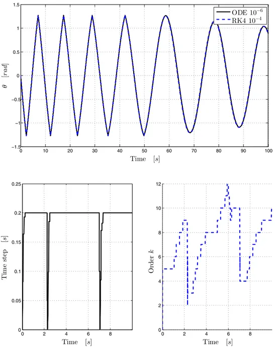
Figure 4 reports the results of two simulations: one uses the Runge–Kutta 4th order solver with a fixed time step of
10−4s and the other relies on the ODE code with a
toler-ance of 10−6. As expected, the ODE solver detects the event
of the contact and reduces the time step and the order of the PECE algorithm, as demonstrated also by Fig. 5.
A comparison of the computational time speed, execut-ing DCAP on the same machine, shows that the PECE solver is 38 % faster than the Runge–Kutta one, in this spe-cific simulation case.
4 Contact
In the aerospace field, offering a range of contact modelling is of crucial relevance for multibody software which aim at tackling the landing of spacecraft on unknown gravel surfaces. Unfortunately, DCAP release 8.0 was lacking this capabil-ity, as it only incorporates a basic elastic contact algorithm between one point and an infinite plane, without soil damping properties and without any tangential friction implementation. 4.1 Contact implementation in DCAP
With the objective of better assisting preliminary assess-ment activities, priority has been given to enhancing Fig. 4 Angle of a pendulum
which hits a surface
0 10 20 30 40 50 60 70 80 90 100 −1.5 −1 −0.5 0 0.5 1 1.5
Fig. 5 Time step and order k of the PECE algorithm of the ODE solver for the first 10 s of the simulation 0 2 4 6 8 0 0.05 0.1 0.15 0.2 0.25 0 2 4 6 8 0 2 4 6 8 10 12
and developing the following three fundamental contact configurations:
–
– “point to infinite plane” contact; –
– “point to finite plane” contact; –
– “point to sphere” contact.
All of them implement the same Hertzian contact formu-lation, based on the following equations:
–
– for the normal direction:
–
– for the tangent directions:
where Fn and Ft are the normal and tangent forces, k is the
stiffness, δ is the penetration depth, c is the damping and µ is the friction coefficient.
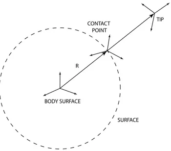
Figure 6 displays that the contact vector is always point-ing from the reference node on the surface (called contact point) to the reference node of the body (called tip): for pla-nar contact types, the vector is perpendicular to the plane, while the vector is normal to the surface of the sphere for the spherical contact.
Figure 5 displays how, in the case of ODE, the detection of the contact is automatic and the computational accuracy depends on the integrator tolerance: once the algorithm
(37) Fn= k · δ3/2+ c · dδ dt (38) Ft= Fn· µ
recognizes the contact event, the integration time step and the order of the algorithm are adapted until the tolerance is matched.
5 Landing simulation
In this Section, the case study of a spacecraft landing on the surface of an asteroid is presented, where the DCAP model is built by taking advantage of all the additional capabilities presented in this paper.
To benchmark and validate the simulation results, an equivalent model has been also built into an independent commercial software (e.g., MSC Adams), where the system has the same properties, and a “point to plane” contact is adopted for the impact with the surface for simplicity.
The spacecraft, as shown in Fig. 7, is composed of a total of five rigid bodies connected with each other: a S/C main body, one sloshing pendulum and three legs. The main body of the spacecraft is linked to the legs by means of 1 DOF translational joints embedding crushable devices. On top of the spacecraft, four thrusters are mounted to push down the lander, after the impact with the surface, with a force of 5 N per thruster.
The total mass of the lander is 362 kg, and the inertia matrix, with respect to its inertial reference frame, is:
[I] = 645.8 6.2 −14.9 6.2 690.1 9.1 −14.9 9.1 628.6 kg m2
Fig. 6 Contact type “point to sphere”
Fig. 7 Lander configuration
Table 3 Pads positions with respect to the S/C CoG
– x (m) y (m) z (m)
Pad 1 0.8877 −1.2968 1.4935
Pad 2 0.8877 −1.2968 −1.4935
Table 3 gives the location of the pads with respect to the CoG of the S/C and Fig. 8 displays two images of the S/C with respect to two perpendicular planes; the overall foot-print diameter is about 3.4 m.
Crushable devices are designed to reduce the shock transmitted to the upper part of the spacecraft by absorb-ing the impact with the terrain [17, 26, 27] and they are modeled as a Coulomb damper, which globally represent
its elasto-plastic deformation. The crushable positions and orientations with respect to the spacecraft CoG are reported in Table 4 and shown in Fig. 8, along the legs of the lander.
Figure 9 shows the characteristics of the crushable devices in terms of displacements and forces. Each device is designed to apply a constant force in the range of 400 N at the interface of the leg to the spacecraft, with a maxi-mum displacement limited to about 20 cm.
Fig. 8 Pads positions with respect to the spacecraft CoG
Table 4 Crushable reference frames positions and
orientations with respect to the S/C CoG – x (m) y (m) z (m) θ1 (°) θ2 (°) θ3 (°) Crushable 1 0.8668 −1.0000 1.4550 −7.4 0.0 4.0 Crushable 2 0.8668 −1.0000 −1.4550 7.4 0.0 4.0 Crushable 3 −1.6532 −1.0000 0.0000 0.0 0.0 −9.0 0 2 4 6 8 10 0 0.02 0.04 0.06 0.08 0.1 0.12 0.14 0.16 0.18 0 0.02 0.04 0.06 0.08 0.1 0.12 0.14 0.16 0.18 −100 0 100 200 300 400 500
The sloshing effect implemented in this DCAP model aims at introducing an equivalent dynamic disturbance to the spacecraft motion at impact, and does not pretend to accurately encompass all the complex fluid-dynamics of sloshing phenomena. Therefore, following simple represen-tations from literature [28], an equivalent pendulum mass is linked to the S/C CoG by means of a torsional springs. The remaining fuel, contributing to the sloshing effect, is estimated 10 kg. The position of the pendulum, as seen in Fig. 8, is at 26.8 mm on Y axis with respect to the S/C CoG with a pendulum length of 150 mm; stiffness and damping values are 10 and 1 N/m.
A contact model “point to sphere” between the pad of each leg and the surface of the asteroid represents a real-istic model of the touchdown. Therefore, the pad has been modeled as a simple point and the CAD pad representation is only for visual effect. Although a fine characterisation of the soil is crucial to obtain more realistic simulations, the lack of data in early design phases lead to use generic val-ues from internal knowhow.
Moreover, the DCAP gravity gradient feature [11] has also been used to include the weak gravitational field of the asteroid body.
At touchdown, the spacecraft is initially rotated of about 10° with respect to the surface and the S/C CoG is at about 2.4 m from it. The leg number 3, as shown in Fig. 7, is the first one to get in contact with the surface.
Figure 10 shows the linear and angular accelerations of the spacecraft during the landing phase. The maximum lin-ear acceleration peak is less than 2.5 m/s2, which is found
in line with requirements in similar cases [29].
Figure 11 compares the linear and angular velocities of the spacecraft evaluated using DCAP and MSC Adams. Both simulations are found in good agreement: at touch-down, the peak values reach about 0.96 m/s for the linear velocity, and 0.43 m/s for the angular velocity, which is found acceptable.
The resulting forces acting on each leg of the S/C are compared in Fig. 12 for both DCAP and MSC Adams mod-els. The overall dynamics of the system during touchdown is well reproduced. The minor differences are due to the contact type assumed for the two multibody models, as the evolution of the local relative impact angle of each pad is slightly different in case of spherical or planar surface. The sloshing mass, which keeps moving for few seconds after the landing is completed, is the main responsible for the oscillations visible in each graph.
6 Conclusion
In conclusion, this paper initially summarizes the most crit-ical features essential for touchdown and landing simula-tions, and focuses on their particular implementation and validation experience inside the European Space Agency’s DCAP software.
Although quaternions avoid the risk of gimbal lock and prove computationally more efficient than Euler angles, the latter ones are still conveniently displayed to users as the standard output in DCAP, thanks to their direct link to physics.
With respect to fixed-step integrators, ODE solv-ers based on PECE algorithm provide ussolv-ers with faster
0 1 2 3 4 5 6 7 8 9 10 −1 −0.5 0 0.5 1 1.5 2 2.5 0 1 2 3 4 5 6 7 8 9 10 −1.5 −1 −0.5 0 0.5 1 1.5 2
solutions and improved accuracy and allow the software developer to harmonize the internal processes by simplify the management of sudden events.
Also, the paper shows that simple contact algorithms combined into a consistent space multibody simulator can adequately provide technical support to the preliminary design activities, such as feasibility studies in a concurrent environment.
As further evidence, the performance of a DCAP-based simulator, including the features introduced in this paper, is compared to MSC Adams in a realistic landing simulation: the outcome confirms that the multibody simulator based on the DCAP tool is computationally advantageous and technically adequate for this type of activities.
Finally, this paper intends to keep raising awareness in the space community towards the advantages of introducing
0 1 2 3 4 5 6 7 8 9 10 −1 −0.8 −0.6 −0.4 −0.2 0 0.2 0.4 0 1 2 3 4 5 6 7 8 9 10 −0.5 −0.4 −0.3 −0.2 −0.1 0 0.1 0.2
Fig. 11 Linear and angular velocities of the spacecraft in DCAP and MSC Adams
0 2 4 6 8 10 −50 0 50 100 150 200 250 300 350 400 450 0 2 4 6 8 10 −100 0 100 200 300 400 500 0 2 4 6 8 10 −50 0 50 100 150 200 250 300 350 400 450
the multibody approach as a fundamental tool for planetary exploration, whenever complex dynamics is involved.
References
1. Yano, H.: The JAXA Minor Body Exploration Working Group. Science, technology and programmatic progress of the japanese team toward the joint Marco Polo Phase-A study. Marco Polo Workshop. Cannes, France (2008)
2. Richter, L., et al.: Marco Polo Surface Scout (MASCOT) study of an asteroid lander for the Marco Polo mission. Daejeon, Korea. In: 60th International Astronautical Congress (2009)
3. Europa Study Team: Europa Lander Mission. JPL D-71990, Jet Propulsion Laboratory (2012)
4. Yano, H., Kubota, T., Miyamoto, H., Okada, T., Scheeres, D., Takagi, Y., Yoshida, K., Abe, M., Abe, S., Barnouin-Jha, O., et al.: Touchdown of the Hayabusa spacecraft at the Muses Sea on Itokawa. Science 312(5778), 1350–1353 (2006)
5. Kawaguchi, J., Fujiwara, A., Uesugi, T.: Hayabusa - its technol-ogy and science accomplishment summary and hayabusa-2. Acta Astronaut. 62, 639–647 (2008)
6. Biele, J., Ulamec, S., Höhe, L.: Preparing for landing on a comet—The Rosetta Lander Philae. In: 44th Lunar and Planetary Science Conference, Texas (2013)
7. Braun, R.D., Robert, M.M.: Mars exploration entry, descent and landing challenges. J. Spacecr. Rockets 44(2), 310–323 (2007) 8. Woods, M., Woods, M., Shaw, A., Barnes, D., Long, D., Pullan,
D.: Autonomous science for an exomars rover-like mission. J. Field Robot. 26(4), 358–390 (2009)
9. CleanSpace. http://www.clean-space.eu/
10. Wormnes, K., Le Letty, R., Summerer, L., Schonenborg, R., Dubois-Matra, O., Luraschi, E., Cropp, A., Krag, H., Delaval, J.: ESA Technologies for Space Debris Remediation. In: 6th IAASS Conference: “Safety is Not an Option”, Montrel (2013)
11. Baldesi, G., Toso, M.: European Space Agency’s launcher multi-body dynamics simulator used for system and subsystem level analyses. CEAS Space J. 3(1–2), 27–48 (2012)
12. Baldesi, G., Voirin, T., Barrio, A.M., Claeys, M.: Methodologies to perform GNC design and analyses for complex dynamic sys-tems using multibody software. In: Holzapfel, F., Theil, S. (eds.) Advances in Aerospace Guidance, Navigation and Control, pp. 431–450. Springer, Berlin Heidelberg (2011)
13. Tasora, A., Negrut, D., Anitescu, M., Mazhar, H., Toby D.H.: Simulation of massive multibody systems using GPU parallel computation. In: 18th International Conference on Computer Graphics. Visualization and Computer Vision, pp. 1–8. Czech Republic, Plzen (2010)
14. Mazhar, H., Heyn, T., Pazouki, A., Melanz, D., Seidl, A., Bartho-lomew, A., Tasora, A., Negrut, D.: CHRONO: a parallel multi-physics library for rigid-body, flexible-body, and fluid dynamics. Mech. Sci. 4(1), 49–64 (2013)
15. Krenn, Rainer, Gibbesch, Andreas: Soft soil contact mod-eling technique for multi-body system simulation. In: Zavarise, Giorgio, Wriggers, Peter (eds.) Trends in Computational Con-tact Mechanics. Lecture Notes in Applied and Computational Mechanics, vol. 58, pp. 135–155. Springer, Berlin Heidelberg (2011)
16. Rhee, H., et al.: Dynamic simulation of the lunar landing using flexible multibody dynamics model. Special Topics on Structural Dynamics, 31st IMAC, vol. 6 pp. 447–453 (2013)
17. Pham, V.L., Zhao, J., Goo, N.S., Lim, J.H., Hwang, D.S., Park, J.S.: Landing stability simulation of a 1/6 lunar module with aluminum honeycomb dampers. Int. J. Aeronaut. Space Sci. 14, 356–368 (2013)
18. Rogers, W.F.: Apollo experience report—lunar module landing gear subsystem—tn d-6850. Technical report, NASA (1972) 19. Hippmann, Gerhard: An algorithm for compliant contact between
complexly shaped bodies. Multibody Syst. Dyn. 12(4), 345–362 (2004)
20. Hippmann, G.: Modellierung von Kontakten komplex geformter Körper in der Mehrkörperdynamik. Ph.D. thesis, Technische Uni-versität Wien Institut für Mechanik und Mechatronik (2004) 21. Cheli, F., Pennestrì, E.: Cinematica e Dinamica dei Sistemi
Multibody, vol. 1. CEA (2008)
22. Kane, T.R., Levinson, D.A.: Dynamics, Theory and Applications. McGraw-Hill, New York (1985)
23. Henderson, D.M.: Euler angles, quaternions and transformation matrices. Technical report, NASA (1977)
24. Shampine, L.F., Gordon, M.K.: Computer solution of ordinary differential equations: the initial value problem. W.H Freeman and Company, San Francisco (1975)
25. Shampine, Lawrence F.: Error estimation and control for odes. J. Sci. Comput. 25(1), 3–16 (2005)
26. Ponnusamy, D., Maahs, G.: Development and testing of leg assemblies for robotic lunar lander. Constance, Germany. In: 14th European Space Mechanisms & Tribology Symposium (2011) 27. Cooper, S., Maahsand, G., Ponnusamy, D.: Development of a
lightweight, energy absorbing soft-landing system for robotic probes. Barcelona. In: 7th International Planetary Probe Work-shop (2010)
28. Fries, N., Behruzi, P., Arndt, T., Winter, M., Netter, G., Renner, U.: Modelling of fluid motion in spacecraft propellant tanks— sloshing. In: Space Propulsion conference (2012)
29. CDF Study Team. Phobos-Moon of Mars Sampe Return Mission. CDF-145(A), ESA, ESTEC (2014)