“P
RIVATEM
EDICALI
NSURANCE ANDS
AVING: E
VIDENCE FROM THEB
RITISHH
OUSEHOLDP
ANELS
URVEY”
A
LESSANDRAG
UARIGLIA ANDM
ARIACRISTINAR
OSSICEIS Tor Vergata - Research Paper Series, Vol. 13, No. 39 October 2003
This paper can be downloaded without charge from the Social Science Research Network Electronic Paper Collection:
http://ssrn.com/abstract=320881
CEIS Tor Vergata
R
ESEARCH
P
APER
S
ERIES
Private Medical Insurance and Saving:
Evidence from the British Household Panel Survey*
Alessandra Guariglia
University of Kent at Canterbury
and
Mariacristina Rossi
University of Rome at Tor Vergata
Abstract
This paper uses the British Household Panel Survey for the years 1996 to 2000 to investigate whether individuals in the UK save for precautionary motives against uncertain medical costs. In particular, we test the hypothesis that those individuals who are not covered by private medical insurance, and who are therefore more exposed to facing unexpected health care expenditures or loss of income while waiting for treatment, tend to save more than those who are covered. According to our findings, which are based on a wide range of econometric specifications, there is a positive association between insurance coverage and saving, suggesting that private medical insurance does not crowd out private saving. This relationship is however weaker in areas where people feel the quality of medical facilities to be poor and in rural areas.
Keywords: Precautionary saving, Private medical insurance. JEL Classification: D12, D91, E21, H51.
* Corresponding author: Alessandra Guariglia, Department of Economics, Keynes College, University of Kent at Canterbury, Canterbury, Kent, CT2 7NP, United Kingdom. Tel: 1227-827412. Fax: 44-1227-827850. E-mail: [email protected].
1. Introduction
The issue of precautionary saving, according to which people save to self-insure against uncertainty is controversial. Many studies have tested this hypothesis, using data from various countries, but while some of them found strong evidence in its favour (Carroll and Samwick, 1997, 1998; Kazarosian, 1997; Merrigan and Normandin, 1996 etc.), others found little evidence or no evidence at all (Guiso et al., 1992; Lusardi, 1997 and 1998; Dynan, 1993 etc.). Most of these studies estimated equations of wealth, saving, consumption, or Euler equations, which included some measure of uncertainty. A test for the significance of the estimated coefficient associated with the uncertainty variable was then performed. A positive and significant coefficient was seen as evidence in favour of the precautionary saving hypothesis1.
It is obvious that the adequacy of this type of test hinges on the appropriateness of the measure of uncertainty chosen. According to Browning and Lusardi (1996), this measure should be observable, exogenous, and should vary significantly across the population. Most of the studies have proxied uncertainty with either the variability of household income (Carroll and Samwick, 1997, 1998; Lusardi, 1997, 1998; Banks et
al., 2001 etc.), or the variability of household expenditure (Dynan, 1993; Guariglia
and Kim, 2001). These measures are however likely to be unreliable, as they contain various elements which can be directly controlled by households2.
1 Banks et al. (2001), Dardanoni (1991), Merrigan and Normandin (1996), and Miles (1997) tested the precautionary saving hypothesis for the UK using data from the Family Expenditure Survey, while Guariglia (2001) and Guariglia and Rossi (2002) used the British Household Panel Survey. All these studies found evidence in favour of the precautionary saving hypothesis.
2 For an illustration of this point, see Carroll et al. (1999) who give the example of a “tenured college professor who, by choice, works only every other summer, and may [thus] have a much more variable annual income than a factory worker, but does not face the uncertainty of being laid off during a recession.” (p.2).
An interesting issue is to evaluate the extent to which individuals save to self-insure against a more specific type of risk: the risk of becoming ill. Like becoming unemployed, becoming ill is liable to cause a potential downturn in the resources available to an individual. A higher risk of becoming ill should hence induce agents to save more for precautionary reasons. However, given the high variability of medical expenses, a more efficient solution would be for individuals to purchase medical insurance. If an individual is covered by insurance, the risk is in fact taken by the insurance company and the individual only has to face the fixed cost of the insurance premium. One should therefore expect to find a lower level of saving among the insured, compared to the non-insured.
Little empirical work has been conducted to measure the extent to which people save to self-insure against uncertain medical costs. The few existing studies focused on the US, and compared the saving behaviour of individuals with health insurance with that of individuals without it. For instance, Levin (1995) and Starr-McCluer (1996) used cross-sectional US micro data to examine the relationship between the demand for private medical insurance and wealth accumulation. The former study only focused on elderly households, and, by analysing the response of insurance holdings to changes in illiquid assets, found evidence of precautionary saving. On the other hand, the latter study, which was based on the 1989 cross-section of the US Survey of Consumer Finances, found a positive association between insurance coverage and household wealth. Gruber and Yelowitz (1999) studied the effects of public health insurance on saving in the US, and found that Medicaid3 eligibility has a sizeable and significant negative effect on household wealth holdings4.
3 Medicaid is a Federal-State health insurance programme for certain low-income and needy people. It covers approximately 36 million individuals including children, the aged, blind, and/or disabled, and people who are eligible to receive federally assisted income maintenance payments. The second main public health insurance programme in the US is Medicare, which covers approximately 39 million
Our objective in this paper is to analyse for the first time, the relationship between saving decisions and private medical insurance coverage in the UK. It must be noted, however, that due to the presence of the National Health Service (NHS), the UK system is rather different from the US system. The NHS is the dominant provider of health care in the UK, with universal provision that is generally free at source. This suggests that all individuals in the UK are insured against unexpected health expenditure. Yet, in spite of the existence of the NHS, a number of individuals prefer to use private health services for which they need to pay5. This is due to the higher
quality characterising private compared to public health provision. For instance, better hospitals and senior doctors are available in the private sector (Propper et al., 2001). In addition, long waiting lists6 are seen as the most important factor, which considerably lowers the quality of the NHS service, and often induces people to purchase supplementary private insurance (Belsley et al., 1999)7. If they become ill, individuals covered by private medical insurance are therefore likely to access a quick treatment, whereas uninsured individuals are likely to face long waiting periods and,
individuals and provides health insurance to people aged 65 and over, those who have permanent kidney failure, and certain people with disabilities. Contrary to the UK, in the US, universal public health coverage does not exist.
4 Also see Kotlikoff (1989), Hubbard et al. (1995), and Palumbo (1999) for theoretical and simulation analyses of the effects of uncertain medical costs on individual saving behaviour. Kotlikoff (1988) incorporates aspects of health uncertainty into a life cycle consumption model and uses the model to examine the implications of different financing mechanisms for health care on macroeconomic saving rates. Hubbard et al. (1995) build a life cycle model that incorporates uncertainty regarding annual earnings, medical expenses, and longevity to study the consequences of a resource-tested Medicaid program for saving decisions by low- and middle-income families. Palumbo (1999) constructs a dynamic, structural model of household consumption decisions in which elderly families consider the effects of uncertain future medical expenses when deciding current levels of consumption. He then simulates the stochastic dynamic model, and estimates preference parameters using panel data on health, wealth and expenditures for retired families.
5 According to Propper (2000), private expenditure on health care in the UK has grown from 9% of total health care expenditure in 1979 to 15% in 1995. Similarly, the use of private health services has increased from 18% in 1991/92 to 22% in 1994/95 (Burchardt et al., 1999).
6 According to Gravelle et al. (2002), in England, in 1997/98, the average waiting time over all specialities was 111 days, and over 1 million patients were waiting for elective surgery in 1996.
7 In the UK, private medical insurance is voluntary and does not remove the entitlement to NHS care. People can either purchase the insurance individually, or participate to a plan offered through their employer (see Belsley et al., 1999).
therefore a higher loss of income during this period8. Moreover, if they become ill, uninsured people who do not trust the NHS or who would prefer a quick treatment might also face unexpected health care expenditures, as they will prefer to use private rather than public health services9. For these two reasons, one would expect uninsured people to save more for precautionary reasons, compared to insured individuals.
We use the British Household Panel Survey (BHPS) for the years 1996 to 2000 to analyse the relationship between saving and private medical insurance. We initially estimate a simple Tobit equation for the decision to save as a function of an insurance coverage variable and various individual socio-economic characteristics. We then account for the panel dimension of our data set by presenting a random-effects Tobit specification. We also check whether the relationship between insurance coverage and saving differs in areas where people feel the quality of medical facilities to be poor and in rural areas. In these areas, people may in fact have stronger incentives to purchase private medical insurance, and this insurance is more likely to crowd out private saving.
The decision to purchase medical insurance is however likely to be endogenous. As stated by Gruber and Yelowitz (1999): “The insurance status is in fact an outcome of the same choice process that determines saving decisions” (p. 1258). In particular, like the decision to save, the decision to purchase medical insurance depends on the perception that individuals have of risk10. Those individuals without health insurance
8 Because primary and emergency care has generally remained within the domain of the NHS, the majority of treatments covered by private insurance in the UK are elective. It is therefore reasonable to assume that the main cost of waiting for treatment is lost income while not being treated, rather than a worse long-term health state.
9 According to the Office of Fair Trading (1996), 20% of patients in the private sector pay for treatment themselves, not being insured. As stated in Emmerson et al. (2000), “direct payment for the use of private medical facilities may, paradoxically, be more advantageous than buying insurance, for certain individuals” (p. 24).
10 In the case in which the insurance coverage is actually paid for by an employer, we cannot really talk of a decision to purchase medical insurance. In this case, the relevant decision can be seen as the decision to join a firm, which offers free private medical insurance.
could in fact have chosen not to purchase the insurance as they are not risk averse. If this were the case, then these uninsured respondents could save less for precautionary reasons than the more risk averse insured individuals (Zeldes, 1989). Similarly, one could find that the insured agents have a higher rather than a lower level of saving, compared to the uninsured, simply because they are more risk averse. We deal with the endogeneity problem in two ways. First, we use an Instrumental Variable (IV) estimation technique, which instruments for the insurance coverage variable in the saving equation. Second, we simultaneously estimate the insurance coverage and the saving equations using a Full Model Maximum Likelihood approach. This specification allows the two equations to be correlated via their error terms, which both contain the unobservable degree of risk aversion of the respondents. Allowing for a non-zero correlation between the two error terms prevents the coefficient on insurance coverage in the saving equation to mistakenly incorporate a risk aversion component.
From a methodological point of view, our analysis improves on previous studies in two ways. First, being based on a panel data set, it allows us to take into consideration unobserved heterogeneity. Second, we take into account the interdependencies between insurance coverage and saving decisions by using a Full Model Maximum Likelihood approach, which allows the error terms in the two relevant equations to be correlated.
In all our specifications, we find a positive association between insurance coverage and saving. This suggests that in the UK private medical insurance does not crowd out private saving. The positive relationship between insurance coverage and saving appears however to be weaker in areas where people feel the quality of medical facilities to be poor and in rural areas.
The rest of the paper is laid out as follows. Section two illustrates our data set and presents some descriptive statistics. Section three lays down the empirical specification of our equation and describes our initial econometric results based on pooled and random-effects Tobit models. Section four presents a series of alternative specifications. Section five discusses how we control for endogeneity, using both an IV Tobit specification and a Full Model Maximum Likelihood approach. Section six concludes.
2. Main features of the data and descriptive statistics
2.1 The data
The data used in this analysis are from the BHPS. The BHPS was designed as a survey of a nationally representative sample of 10,000 adult members of approximately 5,500 households who were interviewed in 1991. The same individuals, together with their co-residents were then followed and re-interviewed in successive waves. Ten waves are currently available, covering the years 1991 to 2000. The survey focuses, in particular, on household characteristics such as their participation in the labour market, their income and wealth, their health, their education, and, more generally, their socio-economic status11.
In each wave, individuals are asked the following question regarding their saving behaviour:
Do you save any amount of your income for example by putting something away now and then in a bank, building society, or Post Office account other than to meet
regular bills? Please include share purchase schemes and Personal Equity Plan (PEP) schemes.
If a respondent answers “yes” to the previous question12, he/she is then asked:
About how much on average do you personally manage to save a month?
The information that is provided in these questions only refers to positive saving. Dissaving in the form of decumulation of financial assets is not considered, which makes the saving variable that we use in our analysis censored at zero13.
In waves 6 to 10, individuals interviewed are also asked the following question regarding private medical insurance:
Are you covered by private medical insurance, whether in your own name or through another family member?
Those respondents who are covered by the insurance in their own name are then asked:
How is this insurance paid for?
The possible answers that can be given are: paid directly, deducted from wages, paid for by employer, and other.
Our empirical analysis is restricted to those individuals aged between 25 and 65, who are in employment14. We excluded those individuals who did not have valid data on saving, private medical, insurance, demographic, and educational variables, and variables relative to their current and expected financial situation15. Finally, as in Alessie and Lusardi (1997), we examined, case by case, potential outliers in our
12 In the remaining part of the paper, we will refer to those respondents who answered "yes" to the saving question as the savers.
13 All the relevant income and saving variables are expressed in 1995 pounds The variables are deflated using the Retail Price Index.
14 These sample restrictions can be justified by the fact that we want to avoid the effects of schooling, retirement, and unemployment on saving. The self-employed are also excluded essentially because it is particularly difficult to distinguish their personal saving from the saving that they invest in their firm. 15 These variables are those that we use as dependent and independent variables in our regressions.
measure of saving, and we excluded the extreme cases from the sample. The sample that we use in estimation is therefore an unbalanced panel made up of 23,093 observations.
2.2. Descriptive statistics
Table 1 presents descriptive statistics on saving behaviour and insurance coverage. Column 1 shows that the percentage of savers in the overall sample is 49.55%. This percentage tends to be higher for individuals with no dependent children, aged either between 25 and 34 or between 45 and 54. It also increases with education and with income.
Column 2 reports the percentages of individuals covered by private medical insurance for various socio-demographic groups. 22.96% of the respondents in the entire sample are covered. The percentage of insured people tends to be higher for respondents with a college degree aged between 35 and 54, and tends to rise with income.
Columns 3 to 6 report the percentages of savers that can be found within the insured and uninsured groups, as well as the amounts saved by these savers. There is a higher percentage of savers among the insured, who also tend to save larger amounts. This pattern holds for the sample overall, as well as for the various socio-demographic groups reported in the Table. The percentage of savers among the insured is 60.80, whereas the corresponding percentage among the uninsured is 46.20. The insured savers tend to save on average £168.20, whereas the corresponding figure for the uninsured is £119.81. Both among the insured and the uninsured, the percentage of savers tends to be higher for the wealthier and the more educated
individuals, who have no dependent children. The savers in these categories also tend to generally save higher amounts.
According to these descriptive statistics, there appears to be a positive association between medical insurance and saving, which would suggest that UK individuals do not tend to save to self-insure against unexpected health care expenditures. Our objective in the next section is to provide more rigorous tests for this conclusion.
3. Econometric specification and main results
3.1. General specification
In our empirical specifications, we initially report Tobit regressions to analyse the determinants of individual saving decisions, and assess the extent to which insurance coverage affects these decisions. We use a Tobit estimation technique, because as mentioned in the previous section, the question that individuals are asked in the BHPS on their saving behaviour only allows for positive or 0 saving as a response. Saving could in principle take negative values, but these negative values are not observed due to censoring. Using the subscript i to indicate the individual and the subscript t to indicate the wave, and denoting with S*it the respondent's true propensity to save,
which is unobservable (latent), the following relationship will hold:
S*it = Xit’β + γIit + vt + eit,
where the observed saving variable Sit is such that:
Sit=S*it if S*it>0
Iit is a dummy variable that takes value 1 if individual i is covered by private medical
insurance in wave t, and 0 otherwise. Xit includes a set of characteristics of individual
i in wave t, which is assumed to affect saving. It includes a quadratic in age aimed at
capturing the curvature of the saving function. Various demographic and educational variables, regional dummies, and dummy variables relative to the individual’s perceived health status are also included16. These variables are generally aimed at capturing differences in preferences. As those respondents who feel their health status to be poor (good) are more (less) likely to become ill in the future, the health-related variables may also be seen as a control for health risk.
Xit also includes the individual's subjectively evaluated financial situation, and
expectations about next year’s financial situation. The expectations variables are included to see whether respondents save to offset future expected declines in income, in accordance with the life-cycle model.
Finally, Xit includes a proxy for permanent income for each individual, given
that there is evidence that saving varies across levels of permanent income, due to the non-homotheticity of preferences (Carroll and Samwick, 1997, 1998)17. We obtained permanent income by taking the fitted values from a random-effects regression of the individual’s earnings on household characteristics, gender, age, age squared, educational dummies, occupational dummies, and interactions of the latter two groups
16 In particular, we include as explanatory variables in our saving equations two dummy variables relative to the respondent’s perceived health status: “health status: good” and “health status: bad”. These variables are constructed on the basis of the health status questions asked in the BHPS. In waves 6 to 8, and in wave 10, this question is:
Please think back over the last 12 months about how your health has been. Compared to people of your own age, would you say that your health has on the whole been excellent, good, fair, poor, or very poor?
In wave 9 of the survey, this question was not asked. The following question was asked instead:
In general would you say your health is excellent, very good, good, fair, poor?
Our “health status: good” dummy is coded equal to 1 if the answers given by respondents to the first question were excellent or good, and if the answers given to the second question were excellent, very good, or good, and as 0, otherwise. The “health status: bad” variable is coded as 1 if respondents answered poor or very poor to the first question, or poor to the second question, and as 0, otherwise.
of dummies with age and age squared (see Carroll et al., 1999, and Kazarosian, 1997, for a similar approach)18.
The error term in Equation (1) is made up of two components: vt, which
represents a time-specific effect, and accounts for possible business cycle effects, and
eit which is an idiosyncratic error term. We take into account the vt component of the
error term, by including time dummies in all our specifications.
3.2. Pooled and random-effects Tobit regressions
We initially estimate Equation (1) using a simple Tobit specification over the pooled sample. The results are reported in column 1 of Table 2. The positive and statistically significant coefficient on Iit, equal to 50.04, shows that there is a strong positive
association between medical insurance and saving, and suggests that insurance coverage does not crowd out private saving19.
In accordance with the life cycle model, saving tends to be higher for respondents who expect their financial situation to deteriorate. It is also higher for those who consider their financial situation as good, or better than expected, for those who are married, who have A levels, who have a higher permanent income, and who perceive their health status as being good. On the other hand, saving tends to be lower for older respondents, for males, for respondents who see their financial situation as bad or worse than expected, and who expect it to improve, and for people who
17 Permanent income can also be seen as a proxy for wealth.
18 We calculated our proxy for permanent income using all the waves available for each individual, i.e. not limiting ourselves to waves 6 to 10, which are the waves we use in the estimation of our saving equations. This is likely to make our measure of permanent income more powerful.
19 One might argue that this association embeds a wealth effect because it is generally the wealthier individuals who are more likely to purchase medical insurance and to save more (see Table 1). However, our regression contains other variables such as permanent income and the financial situation as perceived by the respondent, which are more likely to capture the effect of wealth on saving.
perceive their health status as bad20. Saving also tends to decline with the number of adults and the number of dependent children present in the household.
One problem with the results reported in column 1 of Table 2 is that they might be biased because they do not take into account unobserved heterogeneity. This particular heterogeneity may be thought of, in general terms, as individual differences in some unobserved or unobservable attribute (like tastes), that might affect saving and might consequently cause an omitted variable bias in the pooled Tobit regression. In particular, as noted in Starr-McCluer (1996), there could be unmeasured differences in income between insured and uninsured individuals. Other things being equal, those workers whose employer provides them with medical insurance are in fact likely to get other non-wage incentives as well. The positive association between saving and medical insurance that was found in the pooled Tobit specification might therefore be a consequence of this effect. In column 2 of Table 2, we report the results obtained from the estimation of Equation (1) using a random-effects Tobit specification, which exploits the panel dimension of our data set to control for individual unobserved heterogeneity. This specification differs from the previous one mainly through the structure of its error term, which now takes the following form:
vi + vt + ξit (2)
vi represents an unobservable individual-specific time-invariant effect, which we
assume to be random and captures the unobserved individual heterogeneity; vt
represents a time-specific effect, and ξit is an idiosyncratic error term.
The panel variance component, ρ, which represents the proportion of the
observed total variance of the error term accounted for by unobserved heterogeneity is
20 Since those respondents who feel their health status to be poor (good) are more (less) likely to become ill in the future, the negative coefficient if front of the “health status: bad” dummy and the
precisely determined and equal to 0.506. This suggests that about 50% of all the variance in saving can be attributed to unobserved individual-specific characteristics. The signs and significance of the estimated coefficients obtained using this specification are similar to those reported in column 1, but the coefficients are generally smaller in absolute value, and some of them are no longer significant21. This indicates that the estimates obtained using the pooled Tobit estimator, which did not take unobserved heterogeneity into consideration, were biased. However, the coefficient on the medical insurance dummy (22.08) is still precisely determined. The significantly positive association between insurance coverage and saving, which we obtained in column 1, was therefore not a by-product of not accounting for unobserved individual-specific characteristics. It might be explained by the fact that differences in the risks of facing loss of income while waiting for treatment and/or of facing unexpected health expenditures characterising the insured and the uninsured respondents are not strong enough to justify higher saving for the latter group.
4. Alternative specifications
4.1. Focusing on areas where people feel the quality of medical facilities to be poor and on rural areas.
positive coefficient in front of the “health status: good” dummy provide evidence against the fact that people save to self-insure against health risk.
21 For instance, the coefficients on the “health status: good”, “health status: bad”, “financial situation: bad”, “financial situation expected to improve”, and “A levels” dummies and on the “number of adults” variable, which were precisely determined in the pooled Tobit specification, are no longer significant in the random-effects Tobit specification. On the other hand, the coefficients on the “college degree” and the “postgraduate degree” dummies, which were poorly determined in the pooled Tobit specification are statistically significant in the random-effects case.
We now investigate whether the positive association between insurance coverage and saving that we found is attenuated in those areas where people feel that the quality of medical facilities is poor, or in rural areas, which are notoriously characterised by fewer NHS providers. In these two types of areas, people are in fact more likely to purchase private health insurance, and private health insurance is more likely to crowd out private saving.
We initially focus on those areas where people feel the quality of the medical facilities to be poor. In order to identify these areas, we make use of the following question, which was asked in wave 8 of the BHPS:
I am going to read out a list of facilities and services in your local area. For each one please tell me whether you consider your local area services to be excellent, very good, fair or poor? Medical facilities.
We identify as individuals living in areas with medical facilities of poor quality those respondents who answered “poor” to the above question. We then create a dummy equal to one for those individuals who felt that the quality of medical facilities in their area of residence was poor, and equal to 0 otherwise22. We interact our medical insurance variable with this dummy and add the interacted variable to the original Tobit regression for saving. Our results, presented in column 1 of Table 3, show that the coefficient on the medical insurance dummy is positive and precisely determined, whereas the coefficient on the interaction term is negative and statistically significant23. In terms of magnitudes, the latter coefficient (-101.28) is larger in absolute value compared to the former (62.53). This suggests that in those
22 5.5% of the individuals in our sample regarded the quality of medical facilities in their area as poor. 23 Note that given that the question relative to the quality of the medical facilities was only asked in wave 8 of the BHPS, the estimates presented in column 1 of Table 3 are only based on that particular cross-section.
areas characterised by poor quality medical facilities, taking a private medical insurance crowds out private saving.
We adopt a similar approach to analyse how the relationship between insurance coverage and saving differs in rural, compared to non-rural areas. We make use of a variable, which allocates each individual to the following types of geographic locations: urban England and Wales areas (with population greater than 10,000); semi-rural England and Wales areas (with population between 3,000 and 10,000); rural England and Wales areas; urban Scotland areas; and rural Scotland areas24.
Using the information provided by this variable, we construct a dummy called “rural”, equal to 1 for those individuals living in rural or semi-rural areas, and equal to 0 otherwise. We then estimate a random-effects Tobit regression for saving which includes the insurance coverage variable, and the same variable interacted with the “rural” dummy. The results are presented in column 2 of Table 325. We find that insurance coverage and saving are positively correlated, and that the coefficient on the interaction term is negative, but only significant at the 10% level. In terms of magnitudes, the coefficient on the interaction term is smaller in absolute value than the coefficient on the insurance coverage dummy. This suggests that there is some evidence that the positive association between insurance coverage and saving is slightly attenuated in rural areas.
24 This variable was originally created for waves 1 to 5 of the BHPS using the definitions developed in Chapman et al. (1998). The BHPS team subsequently extended it to waves 6 to 10. In order to identify a rural sub-sample of the larger BHPS sample, different procedures are used for England and Wales, on the one hand, and Scotland, on the other. In both cases, the definitions used are those developed by the relevant government office, i.e. the Scottish Office in the case of Scotland, and the Department of Environment in the case of England and Wales. The classification is made using the 1991 postcode directory. In Scotland, a postcode is considered to be rural if it has a population density of less than 100 persons per square kilometre.
25 Since the identification of the rural sub-sample in the BHPS is based on the 1991 postcode directory, this variable is missing for those individuals living in areas with new postcodes, which could not be matched with the old ones. The sample used in estimation is therefore limited to 20,246 observations.
4.2. Distinguishing between privately purchased and employer provided medical insurance
As medical insurance can be purchased directly, or provided by employers, one could question whether the two types of insurance affect saving in the same way. In order to address this question, we estimate a random-effects Tobit specification for saving, which includes two medical insurance related dummy variables. The first one is equal to 1 if the respondent holds a self-purchased medical insurance, and equal to 0 otherwise; the second one is equal to 1 if the respondent holds an insurance provided for by his/her employer, and equal to 0 otherwise26. The results are reported in column 3 of Table 327. We can see that both insurance variables are positively associated with saving. In order to test whether the effect of the two dummies on saving is statistically different, we conducted a Wald test (Judge et al., 1985), for which we obtained a χ2(1)statistic of 2.79 (p-value: 0.10). This test indicates that the
effect played by the two insurance variables on saving is statistically identical.
4.3 Introducing household dynamics
A possible objection to our main specification is that we do not take into account household dynamics. This might be important because husband and wife are likely to make joint decisions on purchasing health insurance, labour market participation, household composition, and saving. In particular, in the case of health insurance, one individual might be covered under another family member. We take into account household dynamics in two ways. First, in column 4 of Table 3, we report the results of the estimates of a random-effects Tobit equation for household saving rather than
26 In the latter case, the insurance can be either deducted from the employee’s wages or paid for by the employer.
individual saving. The left-hand side variables all refer to either the household or the household head. The results suggest a positive correlation between private medical insurance coverage of the household head and household saving28.
The second way in which we take household dynamics into account is by estimating separate saving equations for married and unmarried people. In this case, excluding from the sample those respondents who are not in employment, and in particular housewives, might give rise to a potential bias in estimation. In columns 5 and 6 of Table 3, we therefore present the results of the estimation of our saving equations conducted on the entire sample (i.e. not limiting the sample to employed respondents) respectively for married and unmarried individuals29. The results suggest that for both categories of respondents, there is a statistically significant and positive relationship between the private medical insurance dummy and saving30. It is worth noting that in both these specifications the coefficient on the health related variables are precisely determined. In particular, the coefficient associated with the “health status: good” dummy is positive, while the coefficient on the “health status: bad” dummy is negative. As those respondents who feel their health status to be poor (good) are more (less) likely to become ill in the future, this can be seen as further evidence against the fact that people save to self-insure against the risk of becoming ill.
27 Note that the question on how the medical insurance is paid for is only asked to those individuals holding the medical insurance in their own name (i.e. not through other family members). This reduces the sample used in estimation to 21,856 observations.
28 We also found a positive association between insurance coverage and saving if instead of using coverage of the household head as our right hand side variable, we used household coverage, where a household is considered covered by private medical insurance if anyone in the household has coverage. 29 Note that in this context, by married respondents, we mean either legally married or cohabiting people. Also note that given that the sample used in estimation also includes people who do not work, we dropped the permanent income variable, as it is not available for those respondents who do not receive a salary.
30 The positive association between insurance coverage and saving also holds if we estimate our random-effects Tobit specification for saving on the entire sample, but without dividing it into married
5. Controlling for endogeneity
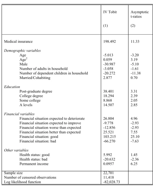
5.1. Instrumental Variables Tobit regressions
The estimates reported so far can be criticised on the ground that they might suffer from a bias due to endogeneity. This would be the case if, for instance, those risk-averse individuals who tend to save generally more, also tend to spend more time and effort to acquire insurance coverage. We take this possibility into account by initially estimating Equation (1) using an IV Tobit specification. We instrument Iit, using
occupational dummies, a variable indicating the size of the individual's workplace, and dummies indicating whether the respondent works in the private sector.
In order to be valid instruments, these variables should be correlated with insurance coverage, but not with saving. As 71% of the individuals in our sample who have the medical insurance in their own name get their insurance coverage through the firms that employ them, it is reasonable to assume that variables characterising these firms are good proxies for insurance coverage. For example, it is well known that larger firms are more likely to offer insurance coverage to their employees. Similarly, managers and professionals are more likely to be covered by private medical insurance provided by their employers than craftspeople31.
Yet, these variables related to the respondent’s workplace are also likely to affect their saving, because for instance managers and administrators or people working for large firms are likely to earn higher wages, and therefore to save more.
and unmarried sub-samples. The results are not reported for brevity, but are available from the authors upon request.
31 Company schemes for which the employer pays the subscription are particularly common among the managers group (ONS General Household Survey, 1995). Our data show that the highest proportion of insured people, 40.7%, can be found in the “Managers and administrators” category, whereas the
However, their effects on saving are indirect, as they operate through an income effect. In our regressions for saving, which already control for the individual’s permanent income and perceived financial situation, it is therefore reasonable to assume that these specific variables will be correlated with insurance coverage, but not with saving. This guarantees that they can be considered as legitimate instruments.
We also performed a formal test of instrument validity, as in Nickell and Nicolitsas (1999). We regressed the insurance coverage variable in our equation on all the exogenous variables plus all the remaining instruments, using a random-effects Probit method. We then tested for the joint significance of the latter instruments, using a Wald test (Judge et al., 1985). We obtained a χ2(10) statistic equal to 287.70
(p-value = 0.00), indicating that the instruments generally have a high explanatory power.
The estimates of our saving equations are obtained using the procedure illustrated in Newey (1987), and are reported in Table 4. Once more, the coefficient on the insurance coverage dummy (149.49) is positive and precisely determined. It is bigger than in the previous regressions, suggesting that the positive association between insurance coverage and saving was not the product of the endogeneity bias. Contrary to the previous specifications, it now appears that the coefficients on all the educational dummies are positive and statistically significant, suggesting that saving tends to increase with educational qualifications. It is also worth noting that the coefficient associated with the “health status: bad” dummy is negative and precisely determined, showing that saving does not increase with health risk. The effects of most of the remaining variables on saving are similar to those previously reported.
lowest proportion, 10.24%, can be found in the “Others” occupational category. 17.31% of people
5.2. Full Model Maximum Likelihood regression
An alternative and generally more efficient way to address the endogeneity of medical insurance coverage is to use a Full Model Maximum Likelihood technique (see Greene, 1991 and Maddala, 1983), which takes into account the interdependence between insurance coverage and saving decisions.
We consider a system composed of both the insurance coverage equation and the saving equation, where saving directly depends on insurance coverage. Denoting with I*it the unobservable (latent) variable indicating the underlying inclination of a
person to possess private medical insurance, our problem can be represented by the following two sets of equations:
I*it = Zit’g + uit,
where the observed medical insurance dummy Iit is such that:
Iit=1 if Iit*>0
Iit=0 if Iit*≤0 (3)
and
S*it = Xit’β + γ I*it + eit = Xit’β + γ (Zit’g+uit) + eit = Wit’δ + ηit,
where ηit = γuit + eit and the observed saving variable Sit is such that32:
Sit=S*it if S*it>0
Sit = 0 if S*it≤ 0 (4)
The determinants of insurance coverage (contained in Zit) are the same as the right
hand side variables of the saving equation (contained in Xit), except for those variables
working in the “Craft related” category are insured.
32 Note that our equation for S
it* contains the latent variable for insurance coverage, rather than the
observed variable. Also note that to keep the notation simple, we did not include any time-specific component in the error terms of Equations (3) and (4). However, we included time dummies in both specifications.
related to the respondent’s past and future expectations about his/her financial situation. The latter variables had been included in the saving equation to test for the presence of life-cycle behaviour. For the reasons outlined in the previous sub-section,
Zit also includes occupational dummies, a variable indicating the size of the
individual's work place, and a dummy indicating whether the respondent works in the private sector33.
We assume that the error terms in the insurance coverage and saving equations (uit and eit) are jointly normally distributed with mean 0 and variance-covariance
matrix
Σ
, where:Σ
= 1 eu ue 2 e σ σ σ . (5)The non-zero covariance between uit and eit allows the shocks to insurance
coverage to be correlated with the shocks to saving34. This correlation reflects the risk aversion term, which is not observed by the econometrician, and is thus incorporated in the error terms of both equations. Allowing for a non-zero correlation between the two error terms prevents the coefficient on insurance coverage in the saving equation to wrongly subsume a risk aversion component, which would make it biased.
Due to the censoring, we can divide our sample into the following four categories:
Category 1: The individuals who save and are insured, such that:
Sit* = Wit’δ + ηit >0 and Iit* = Zit'g + uit > 0.
Category 2: The individuals who do not save and are insured, such that:
Sit* = Wit’δ + ηit ≤ 0 and Iit* = Zit'g+uit > 0.
33 In order for our model to be identified, it is important that the insurance coverage equation includes at least one variable that affects insurance coverage, but not saving (Greene, 1991).
Category 3: The individuals who save and are not insured, such that:
Sit* = Wit’δ + ηit > 0 and Iit* = Zit'g+uit ≤ 0.
Category 4: The individuals who do not save and are not insured, such that:
Sit* = Wit’δ + ηit ≤ 0 and Iit* = Zit'g+uit ≤ 0.
Denoting with φ(.), Φ(.), and Φ2(.) the univariate normal density function, the
univariate cumulative distribution, and the bivariate cumulative function, respectively; with ση2, the variance of ηit and with σηu, the covariance between uit and
ηit, the probabilities associated with each of the four categories can be written as
follows35: Pr(1) = Pr(Sit*)Pr(Iit* > 0 | Sit*) = φ(ηit, ση)Φ − + σ σ η σ σ η η η η 2 2 u it 2 u ' it 1 g Z . Pr(2) = Pr(Sit* ≤ 0)Pr(Iit* > 0 | Sit*≤ 0) = Φ2(-Wit’δ/ση, Zit'g, -ρ). Pr(3) = Pr(Sit*)Pr(Iit* ≤ 0 | Sit*)=φ(η it,ση)Φ − − − σ σ η σ σ η η η η 2 2 u it 2 u ' it 1 g Z . Pr(4) = Pr(Sit* ≤ 0)Pr(Iit* ≤ 0 | Sit* ≤ 0) = Φ2(-Wit’δ/ση, -Zit'g, ρ).
The log likelihood function for the estimation of the parameters g; β, γ, ση, and σηu
takes the following form:
L = ∑ } 1 category { ln Pr(Sit*, Iit* > 0) + ∑ } 2 category { ln Pr(Sit* ≤ 0, Iit* > 0) + 34 Note that the variance of u
it is normalised to 1.
35 The variance of η
it is given by ση2 = σe2 + γ2 + 2γσue, while the covariance between ηit and uit is
∑ } 3 category { ln Pr(Sit*, Iit* ≤ 0) + ∑ } 4 category { ln Pr(Sit* ≤ 0, Iit* ≤ 0) (6)
The results of the Full Model Maximum Likelihood estimation are reported in Table 5. Columns 1 and 2 present the results relative to the equation for insurance coverage. We can see that the probability of having coverage is lower for people who see their financial situation as bad and who have postgraduate qualifications, and is lower the higher the number of adults present in the household. It is higher for married individuals, who have a higher permanent income, and who perceive both their financial situation and their health status as good. It is also higher for individuals who work in large private companies. The coefficients associated with the occupational dummies are generally precisely determined and negative. This suggests that people employed in the categories other than managers and administrators have lower probabilities of being covered36.
Columns 3 and 4 show the results of the Full Model Maximum Likelihood saving regression. Except for coefficients on the educational dummies, which are no longer statistically significant, the results are very similar to those in Table 4. In particular, the coefficient on the insurance coverage dummy (54.17) is still positive and statistically significant. In terms of magnitude, it is now lower than in the IV Tobit case, but higher than in the pooled and random-effects Tobit cases. We can also see that σηu is positive and statistically significant, indicating a strong correlation
between the attitude to save and the attitude to purchase medical insurance. However, even taking into account the interdependencies between insurance coverage and saving decisions, we do not find a substitution effect between saving and insurance. This result is in line with the findings in Starr-McCluer (1996).
6. Conclusions
In this paper we have investigated whether individuals who are not covered by private medical insurance, and who are therefore more exposed to facing unexpected health care expenditures or loss of income while waiting for treatment, tend to save more than insured individuals. Our results based on waves 6 to 10 of the BHPS, and on a variety of econometric specifications, have suggested that this hypothesis generally does not hold. Even by taking into account the possible endogeneity of insurance purchase, we found that insured respondents always have significantly higher saving than respondents without insurance. This relationship is however weaker in areas where people feel the quality of medical facilities to be poor and in rural areas. Although there is evidence that British individuals save to self-insure against unemployment risk, and more in general income risk (Banks et al., 2001; Guariglia,
2002 etc.), they do not appear to use precautionary saving as a device to protect themselves against the risk of becoming ill. This might be due to the fact that, in spite of the numerous criticisms surrounding the quality of its services, the NHS is considered after all as a reliable institution.
References
Alessie, R. and A. Lusardi, 1997, Saving and Income Smoothing: Evidence from Panel Data. European Economic Review 41, 1251-1279.
Banks J., R. Blundell, and A. Brugiavini, 2001, Risk pooling, precautionary saving and consumption growth. Review of Economic Studies 68, 757-79.
Belsley, T., Hall, J. and I. Preston, 1999. The demand for private health insurance: do waiting lists matter? Journal of Public Economics 72 (2), 155-81.
36 “Managers and administrators” is the omitted category.
Browning, M. and Lusardi, A., 1996. Household saving: micro theories and micro facts. Journal of Economic Literature 34, 1797-1855.
Burchardt, T., Hills, J., and C. Propper (1999). Private welfare and public policy. York; Joseph Rowntree Foundation.
Carroll, C., Dynan, K. and S. Krane, 1999. Unemployment risk and precautionary wealth: evidence from households’ balance sheets. Federal Reserve Board Discussion Paper no. 1999-15.
Carroll, C. and Samwick, A., 1997. The nature of precautionary wealth. Journal of Monetary Economics 40, 41-71.
Carroll, C. and Samwick, A., 1998. How important is precautionary saving? Review of Economics and Statistics 80, 410-19.
Chapman, P., Phimister E., Roberts, D., Shucksmith, M., Upward R., and E. Vera-Toscano, 1998. Poverty and exclusion in rural Britain: The dynamics of low income and employment, York Publishing Services.
Dardanoni, V., 1991. Precautionary savings under income uncertainty: a cross sectional analysis. Applied Economics 23, 153-60.
Dynan, K., 1993. How prudent are consumers? Journal of Political Economy 101 (6),
1104-13
Emmerson, C., Frayne, C., and A. Goodman, 2000. Pressures in UK healthcare: challenges for the NHS. Institute for Fiscal Studies, London.
Gravelle, H., Dusheiko, M., and M. Sutton, 2002. The demand for elective surgery in a public system: time and money prices in the UK National Health Service. Journal of health Economics 21, 423-49.
Greene, W., 1991. Econometric Analysis. Macmillan Publishing Company, New York.
Gruber, J. and Yelowitz, A., 1999. Public health insurance and public saving. Journal of Political Economy 107 (6), 1249-74.
Guariglia, A., 2001. Saving behaviour and earnings uncertainty: evidence from the British Household Panel Survey. Journal of Population Economics, 14, 4,
619-40.
Guariglia, A. and Kim, B-Y, 2001. The effects of consumption variability on saving: evidence from a panel of Muscovite households. mimeo, University of Kent at Canterbury.
Guariglia, A. and Rossi, M., 2002. Consumption, habit formation and precautionary saving: evidence from the British Household Panel Survey. Oxford Economic Papers, 54, 1-19.
Guiso, L., Jappelli, T., and D. Terlizzese, 1992. Earnings uncertainty and precautionary saving. Journal of Monetary Economics 30, 307-37
Hubbard, R., J. Skinner, and S. Zeldes, 1995. Precautionary saving and social insurance. Journal of Political Economy 103 (2), 360-99.
Judge, G., Griffiths, R., Hill, R., Lütkepohl, H., and T.-C. Lee, 1985. The theory and practice of econometrics. Second edition, New York: Wiley & Sons.
Kazarosian, M., 1997. Precautionary savings- A panel study. Review of Economics and Statistics 79 (2), 241-47.
Kotlikoff, L., 1989. Health expenditure and precautionary savings. In: Laurence J. Kotlikoff, What Determines Savings? MIT Press, Cambridge, MA.
Levin, L., 1995. Demand for health insurance and precautionary motives for saving among the elderly. Journal of Public Economics 57 (3), 337-67.
Lusardi, A., 1997. Precautionary saving and subjective earning variance. Economics Letters 57, 319-326
Lusardi, A., 1998. On the importance of the precautionary saving motive. American Economic Review Papers and Proceedings 88, 448-53.
Maddala, G., 1983. Limited-dependent and qualitative variables in econometrics.
Cambridge, Cambridge University Press.
Merrigan, P. and Normandin, M., 1996. Precautionary saving motives: an assessment from UK time series of cross-sections. Economic Journal 106, 1193-1208.
Miles, D., 1997. A household level study of the determinants of income and consumption. Economic Journal 107, 1-25
Newey, W., 1987. Efficient estimation of limited dependent variable models with endogenous explanatory variables. Journal of Econometrics 36, 231-50.
Nickell, S. and Nicolitsas, D., (1999). How does financial pressure affect firms?
European Economic Review, 43, 1435-56.
Office for National Statistics, 1995. General Household Survey, London. Office of Fair Trading, 1996, Health Insurance, London: OFT.
Palumbo, M., 1999. Uncertain medical expenses and precautionary saving near the end of the life cycle, Review of Economic Studies, 66, 2, 395-421.
Propper, C., 2000. The demand for private health care in the UK. Journal of Health Economics 19, 855-76.
Propper, C., H. Rees, and K. Green, 2001. The demand for private medical insurance in the UK: a cohort analysis. Economic Journal 111, C180-C200.
Starr-McCluer, M., 1996. Health insurance and precautionary savings. The American Economic Review 86 (1), 285-95.
Taylor, A., 1994. Appendix: sample characteristics, attrition and weighting. In: Buck N, Gershuny J, Rose D, Scott J (Eds), Changing households: The British
Household Panel Survey 1990-1992. ESRC Research Centre on Micro-Social Change, University of Essex
Taylor, M. (Ed), 1999. British Household Panel Survey user manual volume A: Introduction, technical reports, and appendices. ESRC Research Centre on
Micro-Social Change, University of Essex
Zeldes, S., 1989. Optimal consumption with stochastic income: deviations from certainty equivalence. Quarterly Journal of Economics 104, 275-98.
Table 1: Saving and private medical insurance coverage by individuals’ demographic characteristics, age, education and income
% who save (1) % covered by insurance (2) % of insured who save (3) Non-zero average monthly saving of insured (£) (4) % of uninsured who save (5) Non-zero average monthly saving of uninsured (£) (6) All Demographic variables Married/Cohabiting Not married/cohabiting No dependent children One dependent child or more Age 25 – 34 35 – 44 45 – 54 55 – 65 Education Post-graduate degree College Some college A levels
Less than A levels Income First quintile Second quintile Third quintile Fourth quintile Fifth quintile 49.55 50.07 47.58 53.97 43.65 50.28 47.77 51.03 49.21 59.81 58.79 51.66 52.25 43.99 38.16 42.97 49.96 54.07 62.62 22.96 24.25 18.10 22.91 23.04 20.59 25.10 24.12 21.35 26.53 31.38 25.37 24.06 18.37 13.45 15.19 19.00 24.84 42.34 60.80 60.27 63.46 65.79 54.17 61.59 56.72 64.00 65.12 68.00 64.94 61.52 66.56 47.29 51.25 55.06 58.20 59.63 67.42 168.20 166.20 183.67 187.02 140.48 158.39 164.35 178.69 194.73 281.89 241.82 159.89 149.63 52.64 112.76 111.33 118.91 139.61 234.93 46.20 46.81 44.08 50.46 40.50 47.35 44.78 46.91 44.89 56.86 55.98 48.31 47.72 43.72 35.97 40.80 48.02 52.23 59.09 119.81 121.36 114.03 127.60 106.83 119.27 114.51 123.63 129.16 192.83 151.33 125.72 118.75 57.02 80.23 92.48 99.00 128.38 197.65 Source: BHPS, waves 6 to 10.
Table 2: Tobit estimates for saving Pooled Tobit (1) Random-effects Tobit (2) Medical insurance Demographic variables Age Age2 Male
Number of adults in household
Number of dependent children in household Married/Cohabiting Education Post-graduate degree College degree Some college A levels Financial variables
Financial situation expected to deteriorate Financial situation expected to improve Financial situation worse than expected Financial situation better than expected Financial situation: good
Financial situation: bad Other variables
Health status: good Health status: bad
Permanent income
Sample size
Number of censored observations
ρ
Log likelihood function
50.039 (14.66) -6.021 (-3.90) 0.073 (3.98) -46.297 (-8.12) -4.167 (-2.21) -19.190 (-10.90) 13.001 (3.28) 5.705 (0.53) 4.406 (0.60) 3.523 (0.83) 13.709 (2.71) 28.694 (5.36) -7.484 (-2.27) -12.429 (-2.86) 28.230 (8.44) 112.863 (29.03) -73.387 (-8.58) 8.824 (2.16) -20.638 (-2.38) 0.162 (12.58) 23,093 11,652 … -83,172.65 22.082 (10.14) -3.411 (-3.20) 0.0451 (3.57) -12.468 (-3.16) 0.068 (0.06) -7.191 (-5.91) 6.314 (2.41) 22.940 (2.88) 20.114 (3.84) 3.897 (1.32) 5.845 (1.58) 14.657 (5.68) -1.291 (-0.80) -7.483 (-3.76) 14.736 (9.04) 26.848 (13.99) -4.407 (-1.32) 0.596 (0.29) -5.793 (-1.48) 0.079 (9.51) 23,093 11,652 0.506 -140,606.13
Notes: Asymptotic t-ratios are in parenthesis. Regional and time dummies were included in all specifications. “Less than A-levels” is the omitted educational category. “Health status: fair” is the omitted health category. ρ represents the fraction of total variance attributable to the unobserved random-effects.
Table 3: Tobit estimates for saving: alternative specifications (1) (2) (3) Dependent variable: household saving (4) Entire sample: married people (5) Entire sample: unmarried people (6) Medical insurance Medical insurance *poor Medical insurance*rural
Medical insurance: privately purchased Medical insurance: purchased through employer
Demographic variables
Age Age2
Male
Number of adults in household
Number of dependent children in household Married/Cohabiting Education Post-graduate degree College degree Some college A levels Financial variables
Financial situation expected to deteriorate Financial situation expected to improve Financial situation worse than expected Financial situation better than expected Financial situation: good
Financial situation: bad
Other variables
Health status: good Health status: bad
Permanent income
Sample size
Number of censored observations
ρ
Log likelihood function
62.528 (7.76) -101.285 (-3.34) … … … … … … -10.685 (-2.93) 0.132 (3.08) -50.740 (-3.73) -3.490 (-0.77) -16.420 (-3.97) -2.286 (-0.24) -19.907 (-0.76) -6.022 (-0.34) -0.499 (-0.05) 21.077 (1.76) 18.989 (1.49) -11.159 (-1.43) -17.123 (-1.69) 31.702 (4.00) 113.889 (11.87) -56.918 (-2.88) 4.354 (0.48) -33.184 (-1.78) 0.175 (5.72) 3,991 1,949 … -14,753.4 22.756 (8.68) … … -8.106 (-1.65) … … … … -3.350 (-2.93) 0.044 (3.29) -13.218 (-3.12) 0.004 (0.00) -7.589 (-5.77) 6.138 (2.19) 20.055 (2.34) 22.458 (3.98) 3.520 (1.10) 6.425 (1.61) 15.765 (5.68) -0.389 (-0.22) -7.026 (-3.27) 14.821 (8.44) 27.866 (13.54) -4.541 (-1.27) 1.307 (0.60) -4.075 (-0.96) 0.089 (9.47) 20,246 10,240 0.511 -123,417.3 … … … … … 22.028 (6.02) 29.001 (10.22) -3.306 (-3.04) 0.043 (3.36) -13.567 (-3.35) -0.040 (-0.03) -7.238 (-5.84) 6.010 (2.31) 24.851 (3.08) 20.903 (3.90) 4.375 (1.44) 6.501 (1.73) 14.056 (5.29) -1.277 (-0.77) -7.952 (-3.90) 14.340 (8.55) 27.019 (13.80) -4.438 (-1.32) 0.352 (0.17) -5.354 (-1.34) 0.077 (8.99) 21,856 11,106 0.509 -133,040.4 32.811 (7.93) ... … … … … … … … -4.778 (-2.35) 0.0638 (2.68) -22.069 (-2.80) 28,979 (10.86) -14.095 (-6.30) 32.849 (5.94) 34.707 (2.44) 21.845 (2.23) 2.664 (0.48) 10.391 (1.51) 23.207 (4.72) -2.580 (-0.82) -6.760 (-1.78) 23.553 (7.34) 42.333 (11.50) 1.877 (0.30) 2.753 (0.69) -11.929 (-1.47) 0.101 (6.42) 13,143 4,984 0.474 -85,078.9 22.904 (10.96) ... … … … … … … … 2.920 (3.78) -0.34 (-3.93) 16.956 (7.97) -3.209 (-2.56) -8.776 (-8.64) … … 56.162 (8.45) 55.748 (15.09) 18.581 (7.76) 9.635 (2.88) 11.052 (4.67) -2.226 (-1.44) -8.699 (-4.83) 15.747 (10.02) 26.815 (15.12) -2.933 (-1.00) 4.120 (2.24) -7.253 (-2.43) … … 27,823 15,998 0.463 -169,809.1 34.760 (8.32) ... … … … … … … … 5.912 (5.29) -0.066 (-5.17) 20.350 (5.54) 2.508 (1.68) -6.139 (-2.56) … … 69.958 (6.81) 47.021 (8.56) 8.503 (2.08) 15.768 (2.81) 7.984 (2.81) 2.298 (0.83) -7.010 (-2.28) 20.237 (6.99) 33.472 (11.41) -1.792 (-0.47) 7.570 (2.41) -6.187 (-1.35) … … 8,177 5,177 0.460 -49,394.05
Notes: “Poor” is a dummy variable equal to 1 in those areas where people feel medical facilities to be of poor quality, and equal
to 0 otherwise. “Rural” is a dummy variable equal to 1 in rural areas, and equal to 0 otherwise. The estimates in columns 1, 2, 3, and 4 only refer to people in employment. The estimates in columns 5 and 6 are based on the entire sample, which also includes the unemployed and people out of the labour force. The estimates in column 2 are based on wave 8 of the BHPS only, and were
obtained using a simple Tobit specification. The estimates in columns 1, 3, 4, 5, and 6 were obtained using a random-effects Tobit specification. Also see Notes to Table 2. Source: BHPS, waves 6 to 10.
Table 4: Instrumental variables Tobit estimates for saving IV Tobit (1) Asymptotic t-ratios (2) Medical insurance Demographic variables Age Age2 Male
Number of adults in household
Number of dependent children in household Married/Cohabiting Education Post-graduate degree College degree Some college A levels Financial variables
Financial situation expected to deteriorate Financial situation expected to improve Financial situation worse than expected Financial situation better than expected Financial situation: good
Financial situation: bad Other variables
Health status: good Health status: bad
Permanent income
Sample size
Number of censored observations Log likelihood function
198.492 -5.013 0.059 -30.987 -3.058 -20.272 2.877 38.401 18.294 8.868 14.507 26.804 -9.778 -12.856 25.521 103.215 -66.270 5.992 -20.632 0.0957 22,701 11,418 -82,028.73 11.33 -3.20 3.19 -5.10 -1.61 -11.38 0.70 3.31 2.39 2.05 2.85 4.96 -2.93 -2.93 7.55 25.10 -7.63 1.45 -2.36 6.25
Notes: The estimates were obtained using the method illustrated in Newey (1987). The instruments used are occupational dummies, size of the workplace, and a dummy for whether the respondent works in the private sector. Also see Notes to Table 2. Source: BHPS, waves 6 to 10.
Table 5: Full Model Maximum Likelihood estimates for insurance coverage and saving Insurance coverage (1) z-statistics (2) Saving (3) z-statistics (4) Medical insurance Demographic variables Age Age2 Male
Number of adults in household Number of dependent children in household Married/Cohabiting Education Post-graduate degree College degree Some college A levels Financial variables
Financial situation expected to deteriorate
Financial situation expected to improve
Financial situation worse than expected
Financial situation better than expected
Financial situation: good Financial situation: bad Occupation
Professional occupations
Associate prof. & technical Clerical & secretarial
Craft related
Personal & protective services Sales
Plant & machine operators Others
Other variables
Health status: good Health status: bad
Permanent income
Size of the workplace
Private sector … 2.637 -0.0243 -106.291 -5.073 0.297 20.756 -25.796 4.617 5.712 6.523 … … … … 24.323 -19.167 -22.210 -23.505 -11.780 -54.360 -27.063 -31.613 -56.196 -43.364 6.814 1.072 0.713 56.481 46.860 … 1.78 -1.40 -1.49 -3.83 0.24 7.50 -2.50 0.63 1.65 1.80 … … … … 9.91 -3.69 -5.68 -5.69 -2.21 -10.04 -3.69 -4.32 -9.74 -5.15 2.46 0.19 3.69 13.86 19.21 54.172 -5.425 0.065 -33.357 -2.739 -19.768 2.703 33.395 15.959 7.422 13.537 27.991 -8.189 -11.674 26.752 103.347 -64.687 … … … … … … … … 6.113 -20.464 0.105 … … 9.33 -3.33 3.35 -5.27 -1.38 -10.72 0.62 2.76 2.00 1.66 2.56 5.19 -2.46 -2.76 7.94 23.87 -7.16 … … … … … … … … 1.42 -2.26 6.55 … … Sample size
Number of censored observations Log likelihood function
22,701 11,418 -41,055.58 ση2 (st.error) σηu (st.error) 1.925 0.243 (0.058) (0.014)
Notes: The saving equation is estimated jointly with the insurance coverage equation. “Managers and administrators” is the omitted occupational category. ση2 represents the variance of the error term in the saving equation after the insurance coverage equation has been substituted into it (see Equation 4 in the text). σηu represents the covariance between the error term in the latter equation and that in the insurance coverage equation (see Equation 3 in the text). Also see Notes to Table 2. Source: BHPS, waves 6 to 10.