MAORY: wavefront sensor prototype and instrument optical design

(1)

ALMA MATER STUDIORUM

UNIVERSITA' DI BOLOGNA

__________________________________________________________________________ __________________________________________________________________________

Dipartimento di Fisica e Astronomia

Dottorato di ricerca in Astrofisica Ciclo XXX

Tesi di Dottorato

MAORY: wavefront sensor prototype and instrument optical design

Settore Concorsuale di afferenza: 02/C1 – Astronomia, Astrofisica, Fisica della Terra e dei Pianeti Settore Scientifico disciplinare: FIS/05 – Astronomia e Astrofisica

Candidato Mauro Patti Coordinatore Dottorato Francesco R. Ferraro Supervisore Emiliano Diolaiti Co-Supervisore Matteo Lombini __________________________________________________________________________

(2)

(3)

Abstract

MAORY will be the multi-conjugate adaptive optics module for the ELT first light. Its main goal is to feed the high-resolution NIR imager and spectrograph MICADO.

The present Thesis address the MAORY system at the level of optical design and analysis. MAORY is a complex science projects whose stakeholder is the scientific community. Its requirements are driven by the science cases which request high resolution and astrometric accuracy.

In an ideal world without atmospheric turbulence, MAORY optics must deliver diffraction-limited images with very low optical distortions.

The tolerance process is one of the most important step in the instrument design since it is intended to ensure that MAORY requested performances are satisfied when the final assembled instrument is operative.

The baseline is to operate wavefront sensing using six sodium Laser Guide Stars and three Natural Guide Stars to solve intrinsic limitations of artificial sources and to mitigate the impact of the sodium layer structure and variability.

The implementation of a laboratory Prototype for Laser Guide Star wavefront sensor at the beginning of the phase study of MAORY has been indispensable to consolidate the choice of the baseline of wavefront sensing technique.

The first part of this Thesis describes the results obtained with the Prototype for Laser Guide Star wavefront sensor under different working conditions.

The second part describes the logic behind the tolerance analysis at the level of MAORY optical design starting from definition of quantitative figures of merit for requirements and ending with estimation of MAORY performances perturbed by opto-mechanical tolerances. The sensitivity analysis on opto-mechanical tolerance of MAORY is also a crucial step to plan the alignment concept that concludes the arguments addressed by this Thesis.

(4)

(5)

Definitions, Acronyms and Abbreviations

AIV Assembly, Integration and Verification

AS Aperture Stop

ELT Extremely Large Telescope ESO European Southern Observatory DOF Degree Of Freedom

FoV Field of View GS Guide Star HO High Order LGS Laser Guide Star LO Low orders

LOR low-order & reference

MAORY Multi conjugate Adaptive Optics RelaY MCAO Multi-Conjugate Adaptive Optics

MICADO MCAO Imaging Camera for Deep Observations NCPA Non-Common-Path Aberrations

NGS Natural Guide Star OPD Optical Path Difference PS Phase Screen

PSD Power Spectral Density PSF point spread function PFR Post Focal Relay RMS Root Mean Square RON Read Out Noise RSS Root Sum Squared

SCAO Single-Conjugate Adaptive Optics SH Shack-Hartmann

SLM Spatial Light Modulator SNR Signal-to-Noise Ratio

SVD Singular Value Decomposition TBD To Be Defined

TBC To Be Confirmed TS Turbulence Simulator TT Tip-Tilt

TTF Tip-Tilt and Focus WF Wavefront

WFE Wavefront Error WFS Wavefront Sensor

(8)

(9)

1. Background

Atmospheric turbulence has been, for centuries, the limit of any ground based optical/IR instrument. Turbulent mixing of air (lead by large scale temperature fluctuations) generates spatial and temporal variations in the atmosphere refractive index [1].

One of the model to explain how WF aberration are generated by turbulence was proposed by Kolmogorov [2]. This and many other models [3] [4] are based on statistic approach and describe the distribution of the strength of refractive index variations through atmospheric turbulence as a function of height z. This structure function is known as C2

n (z) profile and

models the atmosphere as a superposition of thin turbulent layers at variable height with different strength [5].

Three are the main parameters that characterize atmospheric turbulence and directly drive the design and performance of AO systems:

• The Fried parameter, r0∝ [ λ-2 (cos γ)-1

∫

C2n (z) dz]-3/5, gives the aperture over which there is on average one radian of RMS phase aberration. It could be considered as the spatial scale at which an AO system needs to sample its correction [6].

• The isoplanatic angle, θ0 ∝ (cos γ) r0/h, were h is the height of a turbulence. Isoplanatism describes the angular dependence of optical path variations that deviate by less than one radian RMS phase aberration from each other at the isoplanatic angle. • The coherence time, τ0∝ r0/v, where v is the average wind speed, describes the time scale at which optical path variations deviate by less than one radian RMS phase aberration from each other. τ0 defines the required AO temporal correction bandwidth.

The most basic AO systems is made by one WFS, one DM and a RTC [7]. The AO system tries to correct WF aberrations by measuring the optical path deviations using the WFS. The RTC calculates an appropriate correction, and applies this correction to the DM. This feedback loop runs on frequencies of hundred times a second depending on the requirement set by τ0. The WF sampling carried out by the WFS and the spatial scale at which the DM applies its correction are set by r0.

The WFS is an optical device designed to be sensitive to the WF phase and generally works with a high efficiency photon detector (e.g. Charge-Coupled Device or Avalanche Photo Diode).

(10)

Three types of WFSs are the most used in AO depending on the performances the system has to achieve in terms of dynamic range and sensitivity. These three class of WFSs are:

• The Shack-Hartmann WFS [8] is made by an array of lenslets which define an array of sub-apertures across the pupil and produce an array of spots corresponding to the local WF. The positions of these spots respect to the sub-aperture centre are strictly related to the average WF slope or gradient over the sub-aperture.

• The Pyramid WFS [9] is made by a pyramid prism whose tip is placed on a focal plane. A collimator, after the pyramid, generates multiple pupil images. When an aberrated ray hits the prism on either side of its tip, it appears in only one of the multiple pupils. The intensity distributions in the multiple pupil images are a measure for the WF phase (Verinaud et al. 2005). The pyramid prism is often modulated such that a single ray appears in either of the pupil images. The intensity distribution of the pupil images, integrated over a modulation period, is a direct measure of WF slopes in the pupil. The sensitivity of this WFS depends on the modulation amplitude and can be tuned depending on the observing conditions.

• The curvature WFS [10] is made by an oscillating membrane in the focal plane. It measures intensity distributions in two different planes on either side of the focus, corresponding to the wavefront’s curvature or 2nd derivative (Roddier 1988).

The main role of the RTC is the WF reconstruction from WFS measurements. In practise, RTC deals with the WFS measurement vector v (e.g. all the slopes measured by a Shack-Hartmann sensor) and calculates an appropriate correction vector c in terms of voltages to send to the DM.

The WFS approximately works in linear regime, hence WF reconstruction performed by the RTC can be described by the linear system:

Dc = v + n

where n is the measurement noise usually assumed to be Gaussian and uncorrelated, and D is the interaction matrix between DM and WFS.

(11)

In order to solve for c, the RTC derives a reconstruction matrix R and multiply it with v. Basically, R is the Moore-Penrose pseudoinverse of D, since D is usually degenerate and not directly invertible [5] [11].

The DM is made by an array of actuators which are connected to a thin optical surface that deforms under the expansion of the actuators. Distance between two consecutive actuators is a requirement lead by r0 while, the number of actuators and hence, the DM diameter depends on the conjugation altitude and the telescope aperture diameter.

Any AO system needs at least a single GS to correct the WF in its direction. Such a setup is known as SCAO and achieved excellent performances on different instruments over the last years [12] [13] [14].

The limit of SCAO is the isoplanatic angle, this implies that the instrument PSF is not uniform across the FoV and it is close to the diffraction limit only at GS position.

AO wavefront sensing requires GSs bright enough to reach a good SNR for the WFS measures [1]. In many cases, a bright NGS is not available in the FoV. The probability to find suitable NGS is called sky coverage and it strongly depends on the observational wavelength. For instance, on 8-10 meters class telescopes, NGS with magnitude Mv = 14 is required to

compensate images at 2,2µm wavelength [15].

In this context the potential power of LGS AO, proposed by Foy & Labeyrie [16], is clear. The LGSs are introduced in Section 3 along with the issues related to these artificial sources that has been object of study in Section 4 of this Thesis.

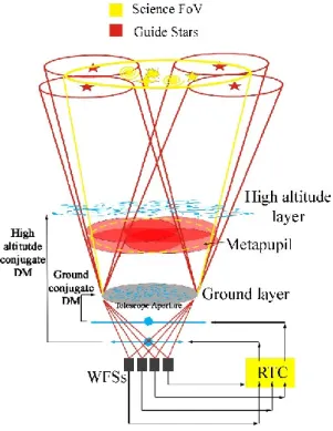
The concept behind the use of LGS is to increase the size of the corrected area by using several GSs to measure the turbulence in the complete 3D volume above the telescope. This field adapted correction, accounting for the field dependence nature of the atmospheric turbulence, is called MCAO [17]. It is a concept that consists in using several DM conjugated in altitude to tune the correction depending on the location in the field.

Of course, one also needs measurements of the turbulence volume. This is obtained by using various WFSs pointing at different field positions, either at NGSs, or at LGSs.

The multiple reference sources are in different directions so that the columns of atmospheric turbulence they probe overlap partially at high altitude and fully at low altitude. Separate DMs, conjugated at specific heights, apply the correction as the sensed turbulence is fully projected on the conjugated layer. In practice, the correction given to each DM has to

(12)

minimise the uncorrected turbulence, both along the atmosphere altitude and in the scientific FoV.

Figure 1 : The MCAO concept. The metapupil is the DM projected diameter to a certain altitude.

The wavefront reconstruction and MCAO control is a complex issue. MCAO correction computation is basically a two-step process:

1. a tomographic reconstruction giving an estimation of the turbulent phase in the volume from multi-channel WFS data. This estimation part depends on GS characteristics (e.g. geometry, flux) and it uses priors on turbulence statistics and its distribution in altitude.

2. a projection of the estimated phase (in the atmospheric volume) onto the DM subspace, accounting for DM characteristics (e.g. number/pitch/altitude). The projection is optimized on a specific FoV.

To improve sky-coverage, sodium LGS constellations are used to measure high orders, with HO WFSs. But since LGSs do not measure tip-tilt, and potentially have difficulties giving an absolute defocus because of sodium profile fluctuations (See Section 3), one also makes use of few NGS to estimate low orders, with LO WFSs.

(13)

2. MAORY. The Multi-conjugate Adaptive Optics RelaY for

ELT

MAORY [18] is the MCAO post-focal module of the ELT [19].

The ELT will use a novel design with a total of five mirrors. The first three aspheric mirrors (M1, M2, M3) form a TMA design [20] for diffraction-limit image quality over the 10 arcminute FoV. The diameter of the segmented primary mirror is approximately 39 metres. The fourth and fifth mirrors (M4, M5) provide AO correction for atmospheric aberrations (M4), and tip-tilt correction for image stabilisation (M5) [21]. These two mirrors can reflect the light toward two Nasmyth platforms at either side of the rotatable telescope

MAORY is designed and built by a Consortium including INAF (Italy) and INSU IPAG (France). ESO is the customer and is also actively involved in the project. It supports the MICADO near-infrared camera by offering two adaptive optics modes: MCAO and SCAO. MAORY and MICADO [22] are placed on the Nasmyth platform A.

MICADO, in imaging, will have two options for the plate/pixel scale: one with ~1.5 mas/px and FoV diameter ~ 20arcsec, and one with ~3-4 mas/px and full 53'' x 53'' FoV. It will be equipped with a large set of broad (I, Z, Y, J, H, K) and narrow band filters. MICADO will also have a coronographic mode and it will allow long-slit spectroscopy (slit orientation along the parallactic angle) with spectral resolution R ~ 4000 - 8000.

The MCAO mode is based on up to six LGSs and three NGSs for WF sensing. In particular, HO WF sensing is performed by using LGSs while LO WF sensing is performed by using NGSs to measure the modes which cannot be accurately sensed by the LGSs. The six LGSs are produced by excitation of the atmospheric sodium with six laser beacons propagated from the edges of ELT pupil. The laser beacons work at wavelength of 589.2 nm and excite the sodium layer by optical pumping of the mesospheric sodium atoms.

At first light, MAORY will contain a single DM with provision for a second DM as an upgrade.

In the MCAO mode, at least one DM within MAORY works together with the telescope M4 while M5 is used to perform only the TT wavefront correction.

The two or more DMs are conjugated to different altitudes to provide a wide FoV with high Strehl ratio and uniformity of the PSF.

The current baseline optical design of MAORY is based on six mirrors (including one or two DMs) and a dichroic beam-splitter. This dichroic beam-splitter is used to split the science

(14)

light from the LGS light that is transmitted to the LGS WFSs by means of a focusable objective [5]. MAORY optics are optimized for the spectral band between 0.8 µm and 2.4 µm and the current optical design is shown in Figure 25.

In MCAO mode, MAORY is required to provide an unvignetted corrected field of diameter D ≈ 75 arcsec for MICADO and an unvignetted field of diameter D ≤ 200 arcsec for the second instrument. The AO correction will be performed over the whole D ≤ 200 arcsec FoV, although the performance is expected to decrease at the edge of the field.

The NGS patrol field may be approximately depicted as the annulus enclosed between D ≈ 75 arcsec and D ≤ 200 arcsec.

The size of outer diameter of NGS patrol field is currently under study and will depend by the sky coverage.

Within this patrol field, three probes (small movable pick-off mirrors) will pick the light from three suitable NGSs to perform LO WF sensing in MCAO mode. In principle MAORY can work with less than three NGSs, with lower performances.

The post focal DMs optical conjugates, inside MAORY, are planned to be at 4km and 15.5km altitude. The LGSs are used for HO wavefront sensing and they are projected from the telescope side on a circle not greater than 2 arcmin angular diameter. The dichroic beam-splitter response curve may be a low-pass filter, with cut-off at about 600 nm, or a notch filter centred at the LGS wavelength. The light reflected by the beam-splitter propagates through the last segment of the main path optics (science path) to the exit port. At the exit port, the MAORY exit focal plane is delivered to MICADO through the so-called Green Doughnut [23].

The Green Doughnut is the interface between MICADO cryostat and MAORY exit focal plane. It’s a cylinder of 800 mm high and 2.6 m in diameter and hosts the SCAO and MCAO subsystems that works with NGSs.

The light picked up by the NGS probes will be split by a dichroic into two beams: • Beam with wavelengths approximately spanning the R and I bands • Beam with wavelengths approximately spanning the H band

Each beam feeds an independent set of WFSs:

• Three NGS WFS approximately spanning the R and I bands • Three NGS WFS approximately spanning the H band

(15)

These two WFS channels will take care of different components of the low order aberrations. NGS WFSs, working in the H band, are used for fast TT and focus corrections with frequencies ~500Hz while the so called LOR WFSs, working in the R and I bands, operate at frequencies in the range 0.1-1 Hz and monitor the LGS NCPA not sensed by the LGS WFS and discussed in the next Chapter.

A single NGS wavefront sensor is deployed in the SCAO mode where wavefront aberrations are compensated by the telescope M4 and M5 mirrors. In this case, the DMs inside MAORY are kept at their reference shape. The SCAO mode is expected to provide a better AO correction than MCAO in a small FoV (D ≈ 10 arcsec) surrounding a bright star that will serve as a single NGS. AO simulations shown that NGS at magnitude MV ≤ 12 allow to obtain an

on-axis Strehl Ratio > 0.6 at λ = 2.2 μm [24].

MAORY also offers provision for a second port for a future instrument which is still undefined.

The instrument project entered its phase B in February 2016 and, at the time of writing, the trade-off studies, in preparation to the last phase of the preliminary system requirement review, are approaching the end of the analysis.

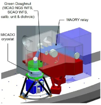
The opto-mechanical design of MAORY has to take care of the tolerance budget described in Section 6.7. The design will be consolidated through an iterative process that will also consider the thermoelastic model and a defined assembly/alignment procedure. A sketch of MAORY-MICADO on the Nasmyth platform is shown in Figure 3.

The MAORY product tree is shown in Figure 2. The instrument is divided into two main parts:

1. Instrument. It is the principal system divided into other sub-systems permanently installed on the Nasmyth platform. It is composed by opto-mechanical components, software and electronics.

2. Auxiliary equipment. It is composed by tools used during the AIT phase and instrument transport.

(16)

MAORY INAF E-MAO-000 AUXILIARY EQUIPMENT INAF E-MAO-A00 MAIN STRUCTURE INAF E-MAO-IM0 INSTRUMENT CONTROL HARDWARE INAF E-MAO-IH0 THERMAL CONTROL INAF E-MAO-IT0

POST FOCAL RELAY OPTICS

INAF E-MAO-IO0

REAL TIME COMPUTER

INAF E-MAO-IR0

LASER GUIDE STAR WAVEFRONT SENSOR

IPAG E-MAO-IL0

NATURAL GUIDE STAR WFS MODULE INAF E-MAO-IN0 AIT TOOLS INAF E-MAO-AE0 TRANSPORTATION CONTAINERS INAF E-MAO-AT0 INSTRUMENT INAF E-MAO-I00 INSTRUMENTATION SOFTWARE INAF E-MAO-IS0

Figure 2 : MAORY product tree

The Post-Focal Relay Optics product in the system-level product tree (Figure 2) is further split into two main sub-products:

• Main Path Optics, which relay the telescope focal plane to the science instrument(s) fed by MAORY;

• LGS Objective, which creates an image of the LGSs, which are used by the MAORY MCAO system for high-order wavefront sensing.

These two sub-products are addressed in this Thesis at the level of optical design and analysis. The Main Path Optics also include one or two post-focal DMs, which are regarded in the studies of this Thesis as plain rigid mirrors. The full design and analysis report of these mirrors is beyond the scope of the Thesis.

The PFR Optics product in the system-level product tree also include the optics mounts and their interfaces to the MAORY Bench. The design and analysis report of these components is beyond the scope of the Thesis.

(17)

Figure 3: Concept of MAORY-MICADO mechanical structure on the Nasmyth platform

2.1 Scientific performance requirements

In MCAO mode, MAORY will have to provide Strehl Ratio SR ≥ 0.3 at λ = 2.2 µm under median atmospheric conditions. This requirement is intended as average value over the MICADO field for observations close to zenith. The requirement has to be achieved over at least 50% of the observable sky at the telescope. The performance goal is SR = 0.5 at λ = 2.2 µm: this performance level may be achievable with a second deformable mirror inside MAORY.

Relative astrometric accuracy is one of the science drivers of the MCAO mode. MAORY will have to permit observations with MICADO such that the relative position on the sky of an unresolved, unconfused source of optimal brightness w.r.t. an optimal set of reference sources is reproducible to within 50 μas (goal 10 μas) over a central field of 20 arcsec diameter (across the entire MICADO field as a goal) over timescales in the range of 1 hour to 5 years.

Concerning relative photometric accuracy, MAORY will have to permit observations with MICADO such that the relative flux of an unresolved, unconfused source of optimal brightness w.r.t an optimal set of reference sources is reproducible to within 0.02 mag (goal: 0.01 mag) across the MICADO field of view over timescales in the range of 1 hour to 5 years.

(18)

(19)

3. LGS WF sensing in the ELT era

Wavefront sensing assisted by LGSs is considered essential for the AO systems of future ELTs to achieve the required performance with high sky coverage.

The fraction of the sky where an efficient AO correction can be achieved is limited by two requirements:

1. GS within the isoplanatic angle of the science target 2. GS bright enough to provide a sufficient SNR for the WFS

In this context, the concept of LGS [16] is a solution to the lack of sky coverage. The use of LGSs, in principle, could substitute bright NGSs, but other difficulties arise. These are linked to the finite distance of LGS from the telescope, its vertical extension and lower atmosphere effects in the upward path of the laser beam.

Roughly speaking, LGS are artificial sources created by the back-scattering of laser light by sodium atoms in the high mesosphere or by molecules and atoms located in the low stratosphere. In the first case, the laser wavelength is tuned to one of the sodium D spectral line and able to excite the sodium layer in the atmosphere at an altitude of about 90km. Sodium atoms are pumped from the ground state into an excited state from which their natural decay produces the desired back-scattered radiation. The second case, the Rayleigh scattering, exploits the elastic scatter of the particles and depends on the atmospheric density which drastically drops with altitude. Rayleigh beacons are less efficient to sample the atmospheric turbulence because they suffer most of the so-called cone-effect, especially for large telescope as ELT. That’s the main reason why the AO correction provided by MAORY LGS WFS is based sodium laser beacon.

The mesosphere contains a build-up of neutral sodium atoms located at a mean height of 90 km (see Figure 5). An ideal LGS should be a point source, but the depth of the sodium layer and its density variability forms an oblate three-dimensional scattering volume with slow variable shape when excited by the laser.

TT are the two lowest order wavefront distortion components which cause the overall image motion in single-aperture AO. To stabilize an image, it is necessary to use a separate reference source that is not twice perturbed by the atmosphere as the LGS case. If the laser is projected and viewed by the full telescope aperture, its motions due to atmospheric turbulence on the upward beam, is added to the same effect resulting in the downward beam. This is valid assuming the wavefront does not change within the propagation time and the result is no

(20)

overall tilt error is detected by a WFS using the same aperture. Besides, as shown in Figure 4, the TT contributions of the upward laser beam and its downward cone are not separable since the latter samples a wider atmospheric area [25].

The current solution to overcome this problem consists in using an additional NGS for TT compensation whose requested magnitude is much higher respect to the pure NGS WF sensing case. For only TT measures, the pupil image can be considered like a SHWFS with only one sub-aperture equal to the telescope aperture increasing the detectable number of photons and thus, the sky coverage.

Figure 4: (Left) Tip-tilt indetermination: when the laser is launched behind the secondary obstruction (or at the side of the primary mirror). The Tip-tilt contributions from the LGS actual position and the atmospheric turbulence cannot be disentangled. (Right) cone effect and MCAO solution to the angular anisoplanatism. At the altitude Hl several LGSs achieve a better coverage of the metapupil, the region at a given altitude inside the

scientific FoV.

A LGS is at finite altitude and its light return samples a cone-shaped volume of the turbulence instead of a cylindric-shaped volume of a source at infinity. For the same reason, the telescope aperture receives a spherical wavefront instead of flat. The laser spot is formed at some finite altitude H above the telescope and a turbulent layer at altitude Hl is sampled differently by

the laser and stellar beams. Besides, the turbulence above H is not sensed by the LGS. The footprint diameter Df for a telescope pupil D is:

Df = D (1-Hl/H)

and the differential extension in the overlap between the LGS and scientific FoV implies that part of the turbulence volume is not sensed.

(21)

The best solution for the cone effect leads to the AO configuration with multiple LGSs. To describe this concept, a metapupil has to be consider as the DM projected diameters:

d = D + 2βHl (β is the angular radius of the FoV)

The beams from scientific objects and guide stars do not sample the whole metapupil, but have smaller footprints. Considering the cone effect, at a defined layer of altitude Hl, the

reconstruction of the turbulence requires more LGSs to sample the same metapupil area respect to the NGS case (Figure 4). It is possible to achieve the same NGS sampling only in the areas where two or more conical beams intersect each other. But, in practice, the WFS measures coming from the LGSs are averaged over the metapupil.

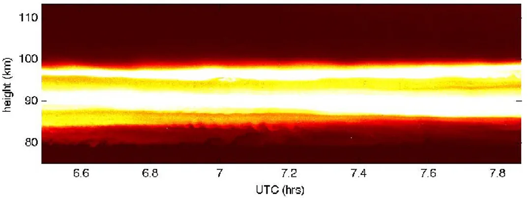
The depth of the sodium layer can vary from 5-20 km depending on location, season, and even time of day [26]. While the origins of sodium atom buildup in the mesosphere is unknown, it has been hypothesized that it was formed from the ablation of meteors [27]. Various groups interested in atmospheric physics have studied this layer, revealing that it is variable in structure and thickness, and occasionally exhibits a multi-modal density in height [28]. (See Figure 5)

This spurious defocus term, due to sodium mean altitude fluctuation, propagates through the AO loop introducing an RMS WFE:

𝜎_𝑑𝑒𝑓2 = 1 16√3

𝐷2 𝐻2∆𝐻

With D telescope diameter and H altitude of sodium layer. Even if this term is induced at a much lower temporal frequency than the atmospheric turbulence defocus, its dependence with the square of the telescope diameter makes critical the possibility to separate the two (e.g. for the ELT). Again, the use of NGS to measure defocus errors, in addition to TT motions, is therefore necessary in the AO systems. For MAORY the reference WFS that will measure the first tens modes of the wavefront, will use the visible light of three NGSs whose near infrared light is instead used to measure the TT and defocus terms (as described in the previous Section).

During the observation, the sky tracking changes the telescope zenith angle γ increasing or decreasing the sodium layer mean distance to the aperture by a factor cos γ. This effect leads

(22)

the focal plane of the LGS to move with time and thus, the AO design must provide the use of a stage that carries the WFS to follow the image position.

3.1 LGS WFS Concept

On the ELT, six sodium LGSs are planned. These are generated by projecting powerful laser beams (589 nm wavelength) from the edge of the telescope aperture up to the natural sodium layer in the mesosphere at about 90 km height. The return light samples the turbulent atmosphere and is collected by a set of WFSs, which measure in real-time the wavefront perturbations due to the atmospheric turbulence.

MAORY contains a PFR, which creates an image of the telescope focal plane (entrance optical interface of MAORY) for the science instrument located on the MAORY exit port. The LGS light is propagated through this relay up to a dichroic beam-splitter, which is located after the deformable mirrors in order to let the LGS WFSs operate in close loop regime. The dichroic lets the light of 6 LGSs, arranged on a circle of about 90” diameter, pass through and reflects science beam and NGS light. Behind the dichroic an objective creates the LGS image plane for the WFSs channel. The LGS WFS will be based on the SH WFS concept.

The current choice of the LGS WFS FoV is 15 arcsec. The detector size is 800x800 pixels, the pixel size is 24µm, the number of apertures is 80x80, the number of pixels per sub-aperture is 10x10 and the ELT sub-sub-aperture size is 0.482m. The choice of LGS WFS FoV greater than 10 arcsec has been done to avoid a large spot truncation (see Section 3.2). This technical requirement implies the need of sub-sampling the LGS image and so to foresee some calibrations to recover a good spot resolution for slope measurement. This is an aspect that has been investigated through a laboratory experiment and discussed in Section 4.

Figure 5: Sodium layer density profile in function of time. ( credit: Paul Hickson, Department of Physics and Astronomy, University of British Columbia.)

(23)

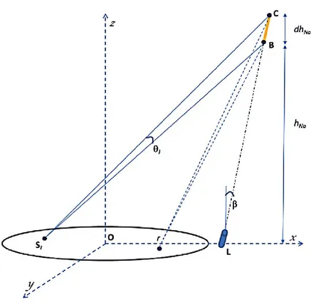
Figure 6 : Geometrical representation of the LGS view from the LGS SH sub-apertures. .

In Figure 6, O is the origin of the xyz reference frame and it is located in the centre of the telescope pupil having diameter = 2𝑟. B and C define the extremities of the LGS region of interest (e.g sodium density profile FWHM when a single Gaussian density profile is considered) and have coordinates in the xyz space respectively:

𝐁 = [ℎ𝑁𝑎 · tan 𝛽𝑥 + 𝑋𝐿𝑇 ; ℎ𝑁𝑎 · tan 𝛽𝑦 + 𝑌𝐿𝑇 ; ℎ𝑁𝑎];

𝐂 = [(ℎ𝑁𝑎 + 𝑑ℎ𝑁𝑎) · tan 𝛽𝑥 + 𝑋𝐿𝑇 ; (ℎ𝑁𝑎 + 𝑑ℎ𝑁𝑎) · tan 𝛽𝑦 + 𝑌𝐿𝑇 ; (ℎ𝑁𝑎 + 𝑑ℎ𝑁𝑎)];

where the coordinates of the Laser Launching Facility are [𝑋𝐿𝑇 ; 𝑌𝐿𝑇 ; 0] and β is the Laser

launching angle.

A generic sub-aperture Si having centre coordinates [Si𝑥 ; Si𝑦 ; 0] sees the LGS under an

angle:

𝜃𝑖 = cos−1 𝑆⃗⃗⃗⃗⃗⃗ · 𝑆𝑖𝐵 ⃗⃗⃗⃗⃗⃗ 𝑖𝐶 ‖𝑆⃗⃗⃗⃗⃗⃗ ‖ ‖𝑆𝑖𝐵 ⃗⃗⃗⃗⃗⃗ ‖𝑖𝐶

(24)

Considering a circular aperture of diameter 𝐷 = 38.542𝑚 and a SH WFS having 80 apertures across the diameter, the worst case in terms of elongation is represented by the sub-aperture at the opposite side of laser launcher position.

3.2 Spot truncation

Figure 7 : LGS Spot truncation. Increasing the distance from the laser launcher position, the sub-apertur see two distinct images. There is a certain position where the finite sub-aperture FoV produces a truncation of the second spot and creates a discontinuity in the slope measurements.

Two sub-apertures placed at different distances from the laser launcher have the same FoV centered at the altitude H but see different segments of the LGS vertical extension. Hence, only the on axis sub-aperture detects the light from any altitude of the LGS. Moving towards the side of the lenslet array, the elongated spot could overflow into the adjacent sub-apertures and thus, it is necessary the use of a field stop whose purpose is to truncate the image of the LGS so that its real vertical extension corresponds to that re-imaged by the most elongated sub-apertures.

An interesting effect arises in the LGS WFS from the combination of the finite WFS FoV and of the sodium profile features. Consider Figure 7 where the sodium density profile has an ideal bi-modal distribution consisting only of two distinct spots separated by a certain altitude

(25)

range. In the LGS WFS sub-apertures close to the laser projection point, the perspective elongation effect is negligible and the two spots are essentially superimposed. If the LGS WFS is focused on one of these two spots, as the distance of the sub-aperture from the laser projection point increases, the two spots produce two distinct images. The one in focus at the centre of the sub-aperture FoV and the other closer to the sub-aperture FoV edge. The centroid therefore shifts away from the sub-aperture FoV centre, in a linear fashion with the distance from the laser projection point, out to a certain sub-aperture where the finite FoV produces a truncation of the second spot. A kind of discontinuity is produced in the centroid measurements (and hence the slopes) across the pupil, translating into more complex wavefront aberrations than pure tip-tilt and defocus. In fact, under the assumption of arbitrarily large LGS WFS FoV, the only wavefront terms related to the sodium layer profile structure and variation would be defocus and, in the case of edge projection, tip-tilt. Because of truncation effects due to the finite LGS WFS FoV, other wavefront aberrations are generated: these are only due to the sodium layer and have no relation with the wavefront aberrations due to atmospheric turbulence that AO system should compensate.

The sodium layer is also characterised by structured and time-variable density profile. Besides, any LGS WFS has finite field of view, typically because of the limited number of pixels of the detector which imposes a trade-off between sampling (i.e. spatial resolution of the imaged LGS spots) and field of view (i.e. extension which can be imaged on the WFS focal plane). The coupled effect of LGS spot truncation and sodium profile temporal variations are spurious and variable wavefront modes, which are only seen by the LGS WFS: their injection into the AO correction loop is detrimental to image quality and therefore an external reference – typically a WFS working on natural stars – is needed for keeping these modes under control. This external reference, independent from sodium layer issues, in MAORY is the so-called Reference WFS provided by an additional channel of the NGS WFS. The preliminary Reference WFS requirements in terms of number of sub-apertures, related to the number of Zernike [29] modes to be monitored, and the sampling time, have been derived using the simplified simulation tool described in [30].

Spot truncation and other LGS issues previously described, have been observed in numerical simulations, but their experimental verification is also deemed essential.

(26)

(27)

4. Laboratory experiment

The experimental work has been conducted by means of a laboratory prototype of a LGS WFS developed at INAF-OAS. The prototype reproduces the expected conditions, in the ELT case, when measuring the wavefront of LGS by means of a SH-WFS.

The laboratory experiment described here has been designed to achieve two main objectives: • Experimental verification of LGS WFS performance under representative conditions

for an ELT

• Supporting the design of the wavefront sensing system of the MAORY instrument for the ELT.

The prototype reproduces the expected conditions, in the ELT case, when measuring the wavefront of LGS by means of a SH-WFS. A simplified version of the prototype was successfully integrated and tested in 2010 [31]. It was able to generate realistic WFS data, including LGS spot perspective elongation and sodium profile features. The prototype has been upgraded [32] [33] to improve the accuracy on the generation of the desired sodium layer and to simulate, not simultaneously, a multiple LGS launching system.

The prototype SH has 40×40 illuminated sub-apertures and the array of spots is re-imaged onto a CCD camera. This WFS order is representative of the E-ELT, considering that the LGS WFS on the E-ELT will have typically 80×80 sub-apertures.

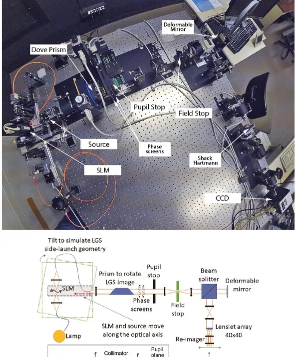
The equivalent sodium layer extension which can be imaged by the prototype is about 20 km in the most elongated sub-apertures, corresponding to about 20 arcsec on the ELT. The conceptual scheme and the experimental setup is shown in Figure 8. The main Prototype SH specifications are listed in Table 1. The light source in the prototype is the output end of an optical fibre, which is fed by an intensity-modulated light pencil: the intensity modulation is applied by a remotely-controlled spatial light modulator (HOLOEYE LC 2002 Transmissive SLM). The SLM is placed between a polarizer and an analyser in the so-called amplitude modulation transmissive mode. This configuration permits the arbitrary choice of transmittance set through 256 values for each SLM pixel (0 = no light ; 255 = full light) in order to simulate a realistic sodium density profile. The output end of the optical fibre and the SLM are both mounted on a motorised linear stage, while the input end of the optical fibre and the optics producing the light pencil feeding the fibre are fixed. The range of motion of the linear stage (about 10 mm) corresponds to the sodium layer extension which can be imaged on the camera. Along the linear stage motion, the output end of the fibre spans the

(28)

full sodium layer extension while the input light pencil crosses different portions of the SLM surface. The axial motion of the source is a variable defocus that translates into a lateral motion of the spots in the WFS sub-apertures. The camera exposure time is set to a few seconds, corresponding to the time necessary for a full span through the sodium layer drawn on the SLM. A tilt of the linear stage travel axis with respect to the prototype optical axis, produces the typical elongation pattern, which is not radial, of a side-launch geometry of the LGS.

The light source module in the prototype includes a Dove prism mounted on a motorised rotation stage whose axis is co-aligned with the optical axis. By changing the position angle of the prism, it is possible to change configuration as if the LGS was launched from a different position around the edge of the telescope which is emulated by the prototype.

Atmospheric-like turbulence may be optionally generated by two plastic screens placed at the aperture stop of the prototype. The screens are mounted on X-Y linear stages to possibly apply temporal evolution.

A field stop is placed at an intermediate focal plane: its diameter can be manually adjusted to introduce different truncations on the LGS images produced by the WFS.

The prototype includes a low-order deformable mirror (ALPAO DM52 with 52 actuators). The purpose of the DM is to introduce low-order and static wavefront aberrations for the test described in Section 4.5. In the remaining test cases, there is no voltage applied to the actuators and the DM surface can be approximated to a flat rigid mirror.

The core of the Shack-Hartmann WFS is a lenslet array, characterised by square geometry, pitch size 300 µm, focal length 3.82 mm.

The array of Shack-Hartmann images is recorded by a scientific-grade CCD camera (pixel size 13 µm, 1k×1k pixels). Each WFS sub-aperture is mapped onto 24×24 pixels of the CCD camera. A re-imager module is necessary to fit the lenslet array pitch with an integer and even number of detector pixels per sub-aperture.

The LGS spots are sampled by 2 pixels per FWHM along the non-elongated axis. Analogue on-chip binning or numerical binning may be used to reduce the sampling to only 1 pixel per FWHM and emulate severe under-sampling conditions.

All the prototype functions are controlled by custom control software coded in C/C++. The software controls all devices (motorised stages, SLM, DM, camera) and manages the

(29)

prototype configuration setup and the acquisition cycles. Data reduction is performed by specific software coded in high-level language IDL®.

Figure 8: Prototype integrated on the optical bench and Prototype conceptual scheme. The axial motion of the source is a variable defocus that translates into a lateral motion of the spots in the WFS sub-apertures. The light intensity modulation is applied by a transmissive SLM. A tilt, respect to the optical axis, simulates the LGS side launch configuration. The prism, rotating around the optical axis, changes the LGS launcher position around the pupil. Phase screens can be placed before the pupil stop. After the DM, conjugated to the pupil, a re-imager module is necessary to fit the lenslet array pitch with an integer and even number of detector pixels per sub-aperture.

(30)

Table 1 : Prototype built-in SH, main specifications Shack-Hartmann specifications

Fully illuminated Sub-apertures 1264 Sub-aperture diameter 300 µm Sub-aperture focal length 3.82 mm Sub-aperture number of pixels 24x24

Pixel size 13µm

CCD camera Read-Out-Noise 11e-

4.1 Common test conditions, limits and calibrations

The Prototype was integrated under a controlled room temperature to reduce thermal fluctuations that effect the system performance. Fixing the temperature at 23ºC, the air conditioning system generates a periodic variation within 1 ºC. This introduces a systematic error in the measures that is translated in global X-Y centroids offset in function of the temperature. The effect is a loss of precision, i.e. a dispersion of a set of WFS images. In terms of RMS WFE, ≈100nm of differential Tip and Tilt terms are introduced while the root sum of squared higher order terms is below 12nm.

Every test was performed in a regime of SNR where the number of photons per sub-aperture (n) stay within 500 and 5000. The laboratory CCD camera has a RON of 15e- _/pixel.

In a CCD RON-dominated:

SNR = 𝑛

√𝑛+𝑅𝑂𝑁2

Scaling the SNR to a typical AO CCD RON of 4e- _{/pixel, the equivalent number of detected}

photon per sub-aperture stay within 360 and 4800.

In SH WFS, at linear regime, centroid coordinates are a direct measure of the local wavefront slope. The Center of Gravity (CoG) is a simple algorithm to estimate the spot position but it is very sensitive to noise. A solution to reduce the noise is to apply a threshold.

The threshold value Th is determined as follows:

(31)

Where T% is the percentage relative to the maximum intensity (max(I)). The threshold

modifies the intensity distribution as follows:

It =

The CoG with a threshold reduces the noise but is still sensitive to the LGS density profile shape and temporal variation. A solution to mitigate these effects is to use the Weighted Center of Gravity (WCoG) [34] algorithm which uses a “reference image'' to evaluate the spot position and it is less sensitive to noise and LGS image intensity variations.

The “reference image'' can be assumed equal to the mean LGS image inside each sub-aperture within a given timescale [35]. The reference acts as a weighted function which reduces the noise effects but introduces an error on the centroid estimation that is proportional to the distance of the actual centroid from the centre of the weighting function. To compensate this error, a calibration curve is empirically derived in each sub-aperture [35].

The prototype experiments didn't consider the temporal aspects of atmospheric turbulence and the LGS image, inside each sub-aperture, has a fixed position. This condition makes negligible any biasing effects due to the weighting function which are not considered. The experimental results, described in this paper, refer only to WFS performance using WCoG centroiding.

Centroid measures were translated in Optical-Path-Difference (OPD) as follows:

{

𝑂𝑃𝐷_𝑥= 𝑑 𝑓 ∆𝑥 𝑂𝑃𝐷_𝑦 = 𝑑

𝑓 ∆𝑦

Where 𝑑 is the lenslet diameter and 𝑓 its focal length. ∆𝑥 and ∆𝑦 are centroid coordinates respect to the sub-aperture centre.

Test results that consider the distribution of sub-aperture OPD are always corrected for the median RMS offset introduced by temperature variations.

I - Th for I ≥ Th

(32)

Test results that consider the distribution of RMS WFE are always corrected for prototype static aberrations that are measured by taking as reference a top-hat sodium profile that does not extend outside the field stop. These corrections on OPD and WFE are a kind of bias subtraction in the resulting data.

To retrieve a wavefront from centroid measures, the followed approach is a modal reconstruction method with Zernike polynomials. The numbers of modes used to fit the wavefront aberrations are 252 Zernike. Further increment on the number of modes results negligible in terms of fit residuals which are within numerical accuracy. Everytime a total RMS WFE is computed, Tip-Tilt and defocus are excluded (Z2 to Z4). MAORY is designed

to work with a reference WFS based on NGSs to monitor low-order wavefront aberrations. Thus, some tests also considered the total RMS WFE for Zernike modes above 54 (Z54) as a

relevant information to support the definition of the requirements of the NGS wavefront sensing sub-system.

The SLM displays a chosen sodium density profile on a grayscale from 0 to 255 levels that is not linear. Any chosen sodium density profile has to be calibrated by the SLM curve response (see Section 4.2).

The Prototype light source, a multimode optical fibre, delivers an output beam whose intensity distribution is approximately Gaussian in shape, involving a gradual drop of the pupil image intensity at its borders. The multimode optical fibre allows the propagation of different light modes whose superposition, at the output end of the fibre, generates lighting inhomogeneities at the pupil stop (see Section 4.2).

Simulated LGS launcher position is on the edge of telescope primary mirror and each sample of images does not consider the temporal aspects of atmospheric turbulence. Given a static sodium density profile, the smallest sample of images, used for the test statistic, contains 100 images. Data reduction takes care of background subtraction, hot pixels, bad lines and cosmic rays. Corrupted pixels values were replaced by the mean of adjacent pixels. Extensive test campaigns have been carried out with the experimental setup. Selected results are shown here.

4.2 End-to-end code verification

The same sodium profiles have been injected into the prototype and, for comparison, into the AO end-to-end simulation code developed for the MAORY instrument project. The MAORY end-to-end simulation code [36] [37] has been designed to accurately model the LGS image

(33)

in the Shack-Hartmann (SH) WFS sub-apertures and to allow sodium profile temporal evolution. The code allows also the simulation of transverse structures, possibly leading to differential effects among the LGSs. The fidelity with which the simulation code translates the sodium profiles in LGS images at the WFS focal plane has been verified using the laboratory Prototype. This test has allowed to verify and to refine the LGS image modelling method implemented in the end-to-end code.

The LGS is an extended light source at a finite distance from the telescope. The LGS image is strongly dependent to perspective elongation given by the laser launcher position relative to the optical axis of a sub-aperture and the longitudinal distance between the LGS and the sub-aperture. We numerically treat the extended LGS as the superposition of portions sliced into planes which are perpendicular to the telescope optical axis. One of the consequences of the cone effect or focus anisoplanatism is that the LGS section at lower layers is nearer the telescope than that at the upper layers and this would cause a stronger intensity at the image plane. Because of geometric optics, the LGS lower layer portions undergo an increase in both magnification and angular deviation of their image positions. On the contrary, for unit increment of LGS altitude, the peak intensity of its image, which undergoes a demagnification, decreases as well as the angular deviation of its image position. After superposing all the LGS portion images, the intensity distribution of a perspective image is determined.

The laboratory prototype requires a calibration procedure to retrieve a correct image from a realistic sodium density profile. Since we use a SLM which displays the density profile in terms of grayscale values, the required process is the follow (see Figure 13):

1. Chose a sodium density profile

2. Calibrate for the SLM curve response. Variations of light intensity are on the grayscale from 0 to 255 levels.

3. Associate the SLM pixels to layer altitudes according to perspective elongation. Since, in the real case, the angular deviation of the image position as a function of a layer altitude is not linear, we have to convert the linear relation between the SLM pixels and the perspective elongation of the SH sub-images peculiar to the Prototype. The differences from simulation are shown in Figure 14 where the relative maximum intensity of each sub-aperture along the pupil diameter (that means with the elongated spot aligned with the pixel grid) are plotted in the case of a LGS image. Due to elongation, we expect that the image peak intensities reach their maximum close to the laser launcher position but, for

(34)

the reasons discussed in Section 0, the Prototype behaves differently. Even if this effect influences the absolute image shapes, it is not important for the scope of every tests since we are interested in relative measures to be cross-checked with the simulations.

The simulated MAORY control scheme is based on three nested AO loops with a different temporal rate [38]. The fasters are for the LGS WFS and a Tip-Tilt Focus Astigmatism (TTFA) NGS WFS which computes the first 5 Zernike modes. The slower is for the Reference WFS. The number and type of WFSs and of DMs can be set as an input of the simulation. In the case of LGS, it is possible to vary the sodium density proﬁle for each simulation step and from one LGS to another.

The flow diagram of the code is shown in Figure 9 where the green box indicates the process that run in open loop (wavefronts generation, including telescope aberrations) and whose outputs, together with the blue box outputs, are used to run the closed loop simulation. The cone effect and the laser up-link propagation are taken into account. The phase screens are computed from the phase (Kolmogorov or Von Karman) Power Spectrum.

An accurate description of the code is reported in [36].

Figure 9 : The simulation code main modules and their interactions. The input parameters are used to build IDL data structures that feed the single modules. The coloured boxes highlight the dependency between the modules. In the first block (green) the wavefronts are generated in open loop and stored; in the second block (blue) mainly the control matrix is computed; then the closed loop takes place (red block); finally, the PSF is computed.

The LGS SH-WFSs are simulated in order to accurately reproduce the projected LGS image in each sub-aperture. It is foreseen the possibility to divide the sodium layer in an arbitrary

(35)

number of sub-layers, in order to take into account for different wavefronts related to diﬀerent sodium layer slices. For each sodium sublayer the step through which each SH sub-aperture is simulated follows this process:

1. The sodium profile portion is projected onto a 2D array having a pixel size that matches one-half of the sub-aperture diffraction limit PSF. This transformation takes into account for the exact geometry of the laser launching system. A 1:1 correspondence between points in the sub-aperture space and points in the sodium profile space is ensured by analytical formulas, starting from a reference altitude that refers to the sub-aperture centre. This reference altitude can change during the simulation according to changes in laser focusing due to zenith angle or to sodium layer variations. Once the pixels that are crossed by the projection of the sodium profile in the sub-aperture are individuated, they are translated into angles under which the profile is seen from each pixel in that specific sub-aperture. Note that the projected profile will intersect the pixel grid defining an irregular grid that depends on the projected profile inclination with respect to the pixel grid, according to the relative position of the sub-aperture respect to the launching laser position.

The value of the pixel that is crossed by the projected profile between two points of intersection is set to the value of the integral of the profile between the altitudes that correspond to the intersection points. This operation is repeated for each of the pixels along the projected profile portion. This computation is done for each considered profile, for all the stars, in open loop and stored in an IDL structure for the closed loop operations. Only the value of the interested pixels is kept in memory.

Figure 10 : The process of sodium profile projection in each sub-aperture is illustrated. a) Hmin and Hmax

(36)

altitude hR centered in the sub-aperture FoV; the black dots along the altitude line represent the altitudes

corresponding to the projection of the points of intersection between the detector pixel grid and the projected profile in the sub-aperture (b). c) shows an example of projected profile in a simulated sub-aperture.

The array size is grater-equal than the sub-aperture FoV multiplied for an integer number given by the final WFS pixel-scale divided by the actual oversampled pixel-scale. The WFS pixel scale is slightly modified in order to be an exact multiple of the diffraction limit pixel size (in the case of MAORY, the diffraction limit pixel size is always smaller than the WFS pixel size). The enhanced FoV is given by the sub-aperture FoV + the size of the long exposure laser image FWHM, in order to avoid the introduction of spurious effects due to truncation.

2. The projected sodium profile portion is then convolved for the long exposure laser PSF. The long exposure laser PSF (that can be either a 2D Gaussian with a given FWHM, or an arbitrary image) is shifted in X and Y by an integer number of pixels corresponding to the integer part of the shift due to the local wavefront tilt (if any). Consequently, the tilt contribution corresponding to that integer shift, is subtracted by the local wavefront. This operation is necessary to avoid the introduction of spurious effects due to the simulation.

3. Now the Field stop can be applied, simply nulling the value of the pixels that fall outside the Field Stop FoV. The Field stop can be set different from the sub-aperture FoV (i.e. smaller).

4. The Diffraction Limited PSF is computed through sub-residual WF Fast Fourier Transform and used as a kernel for the convolution of the array previously computed. 5. This operation is repeated for each profile portion and summed up.

6. The resulting image is re-binned to the ﬁnal WFS pixel scale.

7. The resulting sub-aperture image is summed up to the total WFS image. Note that the sub-aperture image size remains bigger than the size given by the sub-aperture FoV, in order to not cut the image blur due to sub-aperture diffraction.

(37)

Figure 11 : The long exposure laser PSF is shifted in X and Y by an integer number of pixels corresponding to the integer part of the shift due to the local wavefront tilt.

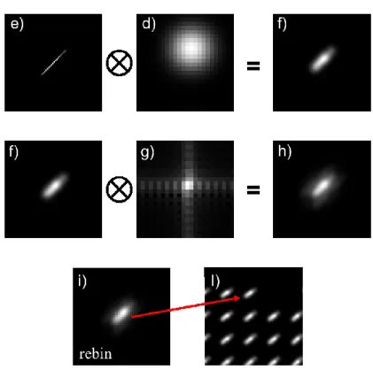
Figure 12 : Simulated LGS WFS image process: the projected sodium profile (e) is convolved for the shifted laser image (d) and then convolved for the sub-aperture diffraction PSF (g). The image (h) is re-binned to the final WFS pixel scale (i) and summed up to the global image (l).

The sodium proﬁle can be changed from one simulation step to the next and from one star to another. For the SH WFS optimization, different algorithms for centroid computation have been implemented (simple center of gravity, center of gravity with a given threshold, weighted center of gravity and correlation). Even the pupil can be updated in order to study effects of mis-registration.

(38)

To compare the LGS images, we used one of the on-sky sodium density profile data from Lick Observatory [39] and run the simulation excluding the atmospheric turbulence and additional sources of noise (i.e. detector noise, background light, photon noise, etc.). In the case of Prototype data, we acquired the images in very high SNR regime so that they are almost noise free. As reference for the comparison, we show in Figure 15 the image of the real sodium density profile as seen by the most elongated sub-aperture along the pupil diameter. The image was converted to one dimensional profile by summing up the pixel values perpendicular to the elongated direction. At this point, the linear Pearson correlation coefficient was used, as parameter, to compare the two profiles resulting from simulation and prototype images. The computed coefficient was equal to 0.97 implying a very high correlation between the two reproduced profiles.

Figure 13 : SLM calibration procedure. To reproduce a realistic sodium density profile in terms of grayscale levels (up-left Figure), the profile has to be calibrated for the SLM curve response (up-right Figure) and finally, the SLM pixels have to be associated to layer altitudes according to perspective elongation (bottom-right Figure). Here the symbols (black circles) follow the image demagnification as the altitude of a LGS portion increases.

(39)

.

Figure 14 : Left: WFS Image of three representative sub-apertures in the pupil. Right: relative maximum intensity of each sub-aperture along the pupil diameter in the case of a LGS image with a side-launch configuration. The Prototype suffers from not uniform pupil illumination.

Figure 15 : Real sodium density profile in function of altitude. This profile is equally seen by the most elongated sub-aperture on the pupil diameter in both cases of Simulation and Prototype data.

(40)

4.3 Wavefront sensor measurement errors

The measurement error at WFS sub-aperture level has been studied for different conditions of SNR, sodium profile and centroid algorithm. In all the cases very good match has been found between experimental results and theoretical expectations derived from numerical simulations. In this subsection, the experimental results refer to a Gaussian sodium profile for three conditions of SNR.

Any centroid algorithms performance is mainly affected by the following sources of error: • Photon noise which follows a Poisson distribution and starts to be significant when

the light intensity is low.

• Background noise which includes hot pixels, bad lines and cosmic rays. • Sampling error which is related to the detector pixels size.

• Fixed pattern noise which is related to the digitization of light intensity by pixels. • Sidelobes of the spot irradiance distribution which depends not only on diffraction but

also on optical surface imperfection (i.e. scratches, dig, bubbles). If the sidelobes symmetry was broken within the centroid searching area, it could cause centroid errors.

In typical LGS images delivered by the prototype is not possible to distinguish these error sources one from the other. For these reasons and many other aspects described in the previous Section, the simulation and prototype data will always be different.

Figure 16 shows the prototype WFS measurement errors in terms of RMS OPDs compared to the theoretical behaviour. Given a sample of images, the RMS OPD of each sub-aperture is the RMS position difference of centroid measurements with respect to the mean.

To assess the performances of WGoC for different levels of SNR, the mean photon counts per sub-aperture is considered as indicator of noise and the distribution of RMS OPD values of the sub-apertures is the performance measure. Figure 16 considers three levels of SNR increasing from SNR-3 to SNR-1. The equivalent number of photon counts per sub-aperture is ≈ 1800 for SNR-3, ≈ 2700 for SNR-2 and ≈ 4700 for SNR-1. Considering a sub-pupil of 0.5m and the LGS WFS operating at 700Hz, these numbers are representative of expected LGS return flux per sub-aperture at ELT site. The three distributions are RMS OPD values of 40x40 sub-apertures. As expected, more photon counts per sub-aperture means a better centroiding accuracy.

(41)

Figure 16 : Measurements performed by WCoG algorithm with a Gaussian sodium density profile. Left: The RMS OPD values of each sub-aperture are the black dots. The theoretical behaviour in function of the distance from laser launcher is the dashed line. Bigger black dots are RMS OPD values of the sub-apertures where the LGS elongation is parallel to the lenslet side. Right: RMS OPD distributions for three levels of SNR. Each box plot is the distribution of RMS OPD values of the sub-apertures. Number of photons per sub-aperture is ≈1800 for SNR-3, ≈2700 for SNR-2 and ≈4700 for SNR-1. Box plots show minimum and maximum values and quartiles.

4.4 Effect of image truncation

Sodium profiles have been injected into the prototype and wavefront sensing has been performed without and with truncation effects. Truncation effects make the WFS detect additional spurious aberrations, especially affecting the first few tens of Zernike modes, which would require a kind of on-line calibration of the LGS WFS measurements by additional reference measurements (e.g. to be performed on NGS).

Figure 17 : Realistic sodium density profile used to evaluate the effect of LGS image truncation. Altitude range (20Km) refers to the maximum sub-aperture FoV (about 20 arcsec).

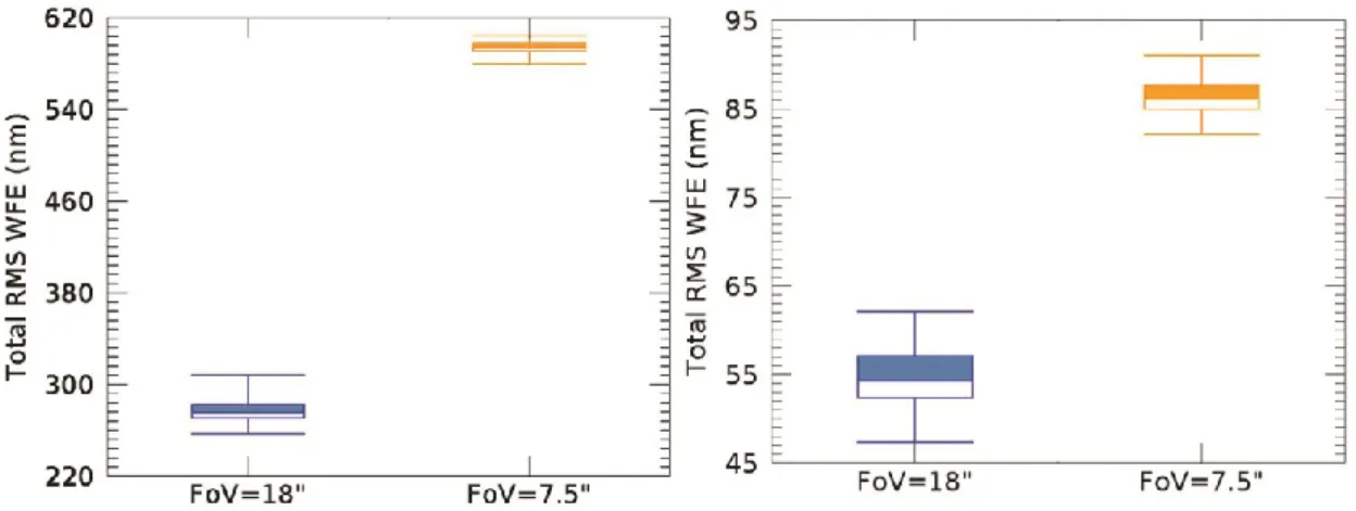
For comparison, we selected a sodium density profile entirely contained in the maximum sub-aperture FoV which is varied by means of a field stop. The following results are related to the sodium density profile shown in Figure 17. The image truncation is symmetric respect the two density peaks. Figure 18 shows the difference in terms of total RMS WFE for

(42)

sub-aperture FoV of 18 arcsec and 7.5 arcsec. Each boxplot is the RMS WFE distribution of all images for a given test condition. Given a sample of WFS images at the same test conditions, each box plot is the RMS WFE distribution of the sample. These results are not influenced by data calibrations described in Section 4.1 since, as already mentioned, the calibration procedure is a kind of bias sustraction of resulting data as shown in Figure 19. The measured wavefronts, with and without image truncation, are not corrected for prototype static aberrations and lead to the same conclusions. The LGS truncation introduces hundreds of nanometers of low-order WFE and it is less significant for modes above Z54.

It has to be considered a loss of photons of about 10% on the entire pupil due to the field stop. The effect of different SNR combined to a fixed level of truncation is the subject of next session.

Figure 18 :WCoG algorithm results described in Section 4.4.. Upper plot: Total RMS WFE above Z4; Lower

plot: Total RMS WFE above Z54. Given a sample of WFS images, these are the distributions of the total RMS

WFE (in nanometers) introduced by the static sodium density profile of Figure 17 for two different FoV. Box plots show minimum and maximum values and quartiles.

(43)

It has to be considered a loss of photons of about 10% on the entire pupil due to the field stop. The effect of different SNR combined to a fixed level of truncation is the subject of next session.

4.4.1 Truncation vs SNR

This section evaluates the effect of LGS image truncation compared to different levels of SNR. The selected sodium density profile is entirely contained in the maximum sub-aperture FoV which is varied by means of a filed stop.

Figure 20 : Realistic sodium density profile used to evaluate the effect of LGS image truncation vs SNR. Altitude range (20Km) refers to the maximum sub-aperture FoV (about 20 arcsec).

The following results are related to the sodium density profile showed on the right of Figure 20. The image truncation regards the low end of density distribution. The number of photons per sub-aperture are regulated by changing the source light intensity. Two levels of SNR have been set when there is no truncation while a fixed SNR, that falls between the other two, has been set when truncation occurs.

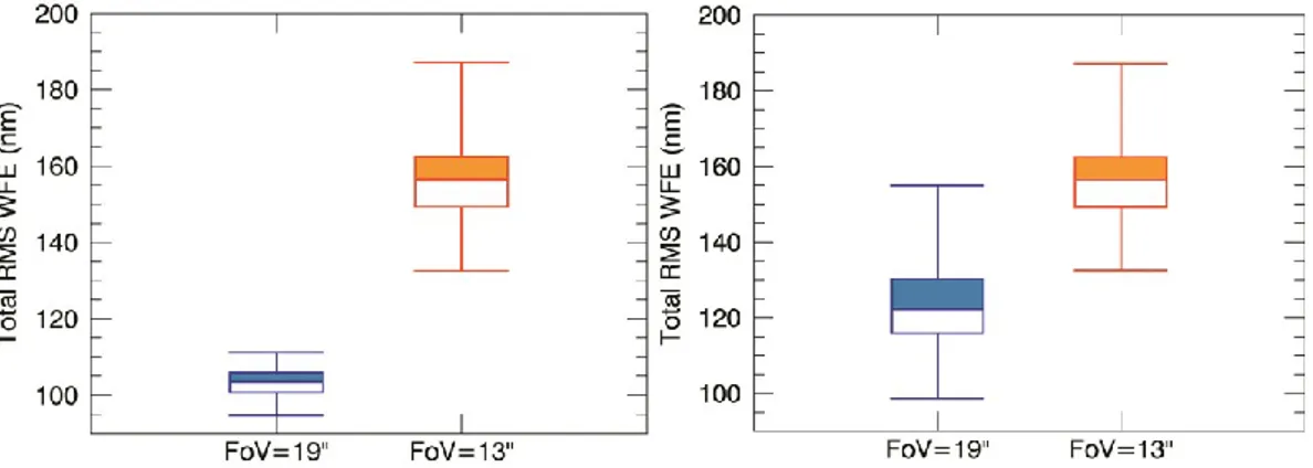
Figure 21 shows the difference in terms of total RMS WFE for a sub-aperture FoV of 19 arcsec and 13 arcsec. Given a sample of WFS images at the same test conditions, each box plot is the RMS WFE distribution of the sample. Blue boxes refer to no-truncated profile whose SNR decreases going from left to right. Orange boxes refer to truncated profile whose SNR is fixed. The effect of reduced SNR translates to greater RMS WFE as well as a wider distribution due to noise. However, the medians of RMS WFE distributions of not truncated cases (blue), are lower than the truncated case (orange).

(44)

Figure 21 : WCoG algorithm results described in Section 4.4.1. Statistical distribution of the total RMS WFE (in nanometer) introduced by the static sodium density profile of Figure 20 for two different FoV. Truncated LGS image is the orange boxplot. Upper plot: Comparison with higher level of SNR of not truncated case (blue); Lower plot: Comparison with lower level of SNR of not truncated case (blue). The box has lines at the lower-quartile, median, and upper-quartile values.

To avoid LGS truncation, for a given number of pixels, the sub-aperture FoV may be increased by under-sampling. However, in this case the WFS loses linearity. Two different approaches are under investigation:

• To calibrate the gain of the centroid algorithm for non-linearity effects introducing a known periodic tilt signal on both axes via a LGS WFS jitter compensation mirrors; • To introduce a blur in the LGS image in order to re-cover Nyquist sampling in the

non-elongated axis, with a negligible effect on the elongated axis.

In the next section, the first approach is explained.

4.5 Effect of image under-sampling

Under-sampled WFS data have been produced by numerical binning of Nyquist-sampled data. Wavefront measurements have been performed on both data sets, using the Nyquist-sampled data as a reference. A centroid gain calibration method has been implemented, based on spot dithering. Under-sampling degrades wavefront measurement performance by up to 25% under the adopted test conditions; the calibration method brings the error down to about 5%. To retrieve the wavefront from centroids measurements, the followed approach is a modal reconstruction with Zernike polynomials. Offsets in terms of centroids translates into residual WFE RMS. To mitigate the effect of under-sampling, the implemented gain centroid calibration procedure is based on spots modulation (i.e. “dithering”) by numerically shifting