The centre cannot hold: patterns of polarization in Nigeria

World Institute for Development Economics Research

wider.unu.edu

WIDER Working Paper 2014/149

The centre cannot hold

Patterns of polarization in Nigeria

Fabio Clementi,

1

_{Andrew L. Dabalen,}

2

_{Vasco Molini,}

2

_and

Francesco Schettino

3

1_{University of Macerata;} 2_{World Bank;} 3_{Second University of Naples; corresponding author: fabio.clementi@unimc.it}

This paper has been presented at the UNU-WIDER ‘Inequality—Measurement, Trends, Impacts, and Policies’ conference, held 5–6 September 2014 in Helsinki, Finland.

Copyright © UNU-WIDER 2014 ISSN 1798-7237 ISBN 978-92-9230-870-4

Typescript prepared by Judy Hartley for UNU-WIDER.

UNU-WIDER gratefully acknowledges the financial contributions to the research programme from the governments of Denmark, Finland, Sweden, and the United Kingdom.

The World Institute for Development Economics Research (WIDER) was established by the United Nations University (UNU) as its first research and training centre and started work in Helsinki, Finland in 1985. The Institute undertakes applied research and policy analysis on structural changes affecting the developing and transitional economies, provides a forum for the advocacy of policies leading to robust, equitable and environmentally sustainable growth, and promotes capacity strengthening and training in the field of economic and social policy-making. Work is carried out by staff researchers and visiting scholars in Helsinki and through networks of collaborating scholars and institutions around the world.

UNU-WIDER, Katajanokanlaituri 6 B, 00160 Helsinki, Finland, wider.unu.edu

The views expressed in this publication are those of the author(s). Publication does not imply endorsement by the Institute or the United Nations University, nor by the programme/project sponsors, of any of the views expressed.

Abstract: Our hypothesis is that Nigeria is going through a process of economic polarization. An

analysis of this type is new for Nigeria; the limited availability of comparable data has hindered an investigation that requires data series not too close in time. The present paper tries to overcome this limitation by making use of recently developed survey-to-survey imputation techniques. To explore polarization, our study uses instead the relative distribution methodology. Findings confirm the sharp increase of polarization. Compared to 2003 consumption distribution is more concentrated in upper and lower defiles, while the middle defiles are progressively emptying out.

Keywords: Nigeria, consumption expenditure, inequality, polarization, relative distribution JEL classification: C14, D30, D63

Acknowledgements: The authors acknowledge financial support from the World Bank. Earlier

drafts of this paper were presented at the If Centenary Conference on ‘Fair and Sustainable Prosperity in the Global Economy’ (Kiel, Germany, 13-14 June, 2014), the Annual Bank Conference on Africa themed ‘Harnessing Africa’s Growth for Faster Poverty Reduction’ (Paris, France, 23-24 June, 2014), and the UNU-WIDER Development Conference on ‘Inequality— Measurement, Trends, Impacts, and Policies’ (Helsinki, Finland, 5-6 September, 2014). We are grateful to all the participants for their useful comments. We also thank Federica Alfani (FAO— Food and Agriculture Organization of the United Nations), Rose Mungai (World Bank—Poverty Reduction and Economic Management Unit) and Ayago E. Wambile (World Bank—Poverty Reduction and Economic Management Unit) for excellent assistance with data preparation. Completion of this work would have not been possible without them. Last, but not least, we thank Christoph Lakner (World Bank—Development Research Group) for comments on an earlier version of the manuscript. Of course, we are solely responsible for all possible errors the paper may contain.

1

1 Introduction

Despite a stable and sustained growth, according to official numbers poverty reduction in Nigeria has not been up to general expectations. Poverty seems to have declined faster in the coastal south and around the federal capital, Abuja. Not every state improved. On the contrary, a large belt of northeastern states have experienced a significant increase in poverty. The lack of a faster reduction in poverty despite a significant growth in gross domestic product (GDP) may be due to a fast rise in inequality (World Bank 2013).

An increase in inequality is, however, just one aspect of the whole problem. Our hypothesis is that Nigeria is also undergoing a process of increasing income polarization. Whereas inequality is the overall dispersion of the distribution, referring to the distance of every individual from the median or mean income, polarization is the combination of divergence from global and convergence on local mean incomes.

In income-polarized societies, people cluster around group means and tend to be far from the mean/median of the overall distribution. Within each group there is income homogeneity and often reducing income inequality: we can talk, thus, of ‘increasing identification’. Between the two groups, instead, we talk of ‘increasing alienation’ (Duclos et al. 2004). The combined effect of alienation and identification forces between two significantly sized groups leads to effective opposition, a situation that might give rise to social conflicts and tensions (Esteban and Ray 1999, 2008, 2011). Also, the group at the top of the distribution has voice while the other group, at the bottom, is voiceless in matters that affect their welfare and the society at large.

Another important aspect of the income polarization analysis is that it is concerned with the disappearance or—as in the case of Nigeria—non-consolidation of the middle class. This precisely occurs when in a society there is a tendency to concentrate in the tails, rather than the middle, of the income distribution. A well-off middle class is important to every society because it contributes significantly to economic growth, as well as to social and political stability (Easterly 2001; Pressman 2007). Also, the middle class constitutes the backbone of democracy (Birdsall 2010) and is a key ingredient in guaranteeing sustainable economic growth and poverty reduction efforts in the long term.

Nigeria represents an interesting case for undertaking a polarization analysis. As mentioned before, GDP and per capita income have grown steadily in the last decade; after GDP re-basing Nigeria is likely to become the biggest African economy and yet clear signs of consolidation of a national middle class are limited. Moreover, the country is increasingly affected by sub-regional conflicts driven to a large extent by disaffected (alienated) groups.

Studies on polarization in Nigeria are few and have approached the relevant issues in a restrictive way. The limited attention paid to long-run patterns could have been due to data problems. Aigbokhan (2000) used the Wolfson (1994) polarization index and provided estimates for the country’s urban and rural areas under national, male-headed, female-headed, and zone dimensions. Aigbokhan (2000) found a higher degree of polarization in the rural areas in the 1990s, and while polarization increased in the country between 1985 and 1992, it declined in the rural areas, which is in contrast with the general belief of increased polarization.

2

Araar (2008) analysed the 2003/04 round of the National Living Standard Survey (NLSS), and tried to identify the main drivers behind polarization in the 1990s by comparing Nigeria to China. Using the same set of data, Awoyemi and Araar (2009) decomposed the Duclos-Esteban-Ray (DER) index of polarization (Duclos et al. 2004). Main results indicate a clear prevalence of the identification component vs. alienation, leading authors to hypothesize the existence of an ongoing polarization process. Also, they identify as main drivers of polarization the increasing divide between macro zones, education, and levels of occupation. The urban/rural divide is found to be insignificant. Awoyemi et al. (2010) extended the analysis looking at the polarization dynamics over the longer time span 1996-2004. Using data from two different household surveys, they find a reduction in polarization using both the Foster and Wolfson (1992) and DER indices: from 0.30 to 0.25 and from 0.44 to 0.38, respectively. They also show that in the southern macro areas (southeast and southwest) indices do not vary significantly. Ogunyemi and Oni (2011) and Ogunyemi et al. (2011) calculated the same indexes on households in rural areas only from 1980 to 2004, finding a similarly decreasing trend. More recent studies like Ogunyemi (2013) indicate a general invariance, with a limited tendency towards increase, by comparing the 2003/04 round of the NLSS and the 2009/10 round of the Harmonized National Living Standard Survey (HNLSS). The present paper is innovative in several aspects. First, rather than just computing and comparing polarization indexes, we use a non-parametric framework (the ‘relative distribution’ introduced by Handcock and Morris 1998, 1999) and compare income throughout the entire income range. The relative distribution analysis requires at least two comparable survey rounds in order to investigate changes along the entire distribution. Since the lack of comparable surveys has limited the scope of previous work, we use survey-to-survey techniques to produce two fully comparable distributions—and this can be regarded as the second aspect of novelty of the present study. Finally, the flexibility of the relative distribution tool allows an accurate analysis at macro-regional level too. Differently from previous contributions, another goal of this paper is to also document sub-national patterns of polarization. Nigeria is highly heterogeneous, so that drivers of polarization can indeed differ across macro regions. It is also worth mentioning that this focus on macro regions is aimed at preparing the ground for future research on the link between polarization and regional conflicts.

Besides the introduction, the paper articulates in four additional sections. Section 2 presents the data and discusses the imputation strategy we use to obtain comparable data on household consumption. Section 3 outlines the distinctive features of the relative distribution method for analysing economic polarization. Section 4 details the main findings of the study. Section 5 concludes.

2 Data and empirical strategy

The comparison of measures such as inequality, polarization or poverty computed on surveys relatively distant in time more accurately captures, we argue, the effect of structural modifications in income distribution. Excluding cases of sudden shocks, in general these measures tend to move relatively slowly, in particular polarization. For our specific case, since we use measures based on comparison of two distributions, it becomes crucial to use distributions sufficiently distant in time in order to see significant differences.

Comparisons over time, however, can be made difficult or even impossible by changes in data collection methodology (Tarozzi 2007). In particular for what concerns survey data, there is

3

increasing empirical evidence that questionnaire revisions can affect respondents’ response in relevant ways (see for instance Deaton and Grosh 2000, among others). For example, the choice of recall period (7, 30 or x _{days before the interview) or the disaggregation of the expenditure}

items can deeply influence reports on expenditure. Other changes such as the switch from a diary-based collection to a recall-diary-based collection can dramatically change aggregate food consumption expenditures, a relevant component of total expenditures in many developing countries.

Beegle et al. (2010), for example, find that in Tanzania recall modules measure lower consumption than a personal diary, with larger gaps among poorer households and for households with more adult members. Ahmed et al. (2014), looking at Bangladesh data, also find that a switch from diary to recall reduces consumption aggregates simply because households remember their expenses better when entering them regularly in a diary. Therefore, switching the data collection methods from diary to recall likely makes poverty estimates incomparable with those of previous rounds in which consumption data were collected by diary.

In Nigeria, the Nigeria National Bureau of Statistics (NBS) uses the 2003/04 NLSS and the 2009/10 HNLSS to monitor progress in poverty reduction in the country. These surveys are representative at state level, use a month-long diary to collect consumption, and enumerators were in the field over a period ranging from October to September of the following year. NBS also conducts other household surveys, most notably the General Household Survey (GHS) cross-section and panel.

The GHS cross-section is a survey of 22,000 households carried out periodically throughout the country. It is freely downloadable from the NBS’s website upon request. Available datasets include six rounds, from 2004/05 to 2010/11. Enumerators visit households once, generally in March, and ask a very standard set of questions. Data on consumption are collected by asking the household about broad categories of consumed items in the last month: food, healthcare, school, and so forth. In 2004/05 and 2010/11 data on consumption were not collected.

The GHS panel is a randomly selected sub-sample from the GHS cross-section consisting of 5,000 households. The panel covers the period 2010/11 (Wave 1) and 2012/13 (Wave 2). It is representative at national and zonal (geopolitical) levels.1 _{Besides the questions asked in a normal}

GHS survey, it contains data on agricultural activities and other household income activities. Consumption data are collected using a seven-day recall period. In every panel wave, households are interviewed twice: once in the ‘post-planting’ period, ranging from August to November, and once in the ‘post-harvesting’ period, ranging from February to April.

Consumption data—the welfare measure we use for our analysis—from these three different sources are not directly comparable. Preliminary results based on poverty and inequality figures computed on the GHS panel and the HNLSS indicate that the figures computed using the former look substantially different from those computed on the latter. The need for comparable data requires, thus, some form of homogenization of consumption figures. In a preliminary version of this paper we focused on the 2010-13 panel dataset (Clementi et al. 2014). The main caveat was that a two-year difference was a short period in which to detect substantial modifications in the distribution. In particular, while consumption polarization might vary due to a number of exogenous factors (crisis, shocks, etc.) and we might observe significant differences, more difficult

4

is linking these transformations to specific covariates such as education, labour market access, spatial divide, and so forth.

In order to enable the data comparison over a longer time span (a decade), we employ

survey-to-survey imputation techniques derived from poverty mapping literature (see Elbers et al. 2003,

among others). Specifically, we use Wave 1 of the panel data to impute consumption on the 2003/04 NLSS survey. Given the importance of obtaining accurate estimates that are comparable over time, it is crucial to calibrate models in a year when both household consumption data and non-consumption data are available, and then use the model to impute household consumption data for years when only the non-consumption data are available. As we will discuss in greater detail below, we will use the panel Wave 2 as a benchmark to check the accuracy of our prediction and in a second stage use the same model to impute the 2003/04 data.

The imputation process is a simplified version of the methodology developed in Elbers et al. (2003). Stifel and Christiaensen (2007) provide theoretical guidance regarding the variables to be included in imputation models. They recommend including covariates that change over time, but call for excluding variables whose rates of return are likely to change markedly in the face of evolving economic conditions. Following Stifel and Christiaensen (2007), we included several household durables but excluded mobile phones, as their relationship with total household expenditure has been changing rapidly in the last ten years. In fact, ten years ago ownership of mobile phones was a good predictor of high income; today, such phones are prevalent among the lower- and middle-income classes and even among the poor (Ahmed et al. 2014). Other variables include household characteristics, location, and zone-interacted variables. Most of the variables are significant and show the expected sign, and, more importantly, the model yields a 2

R _{of 0.46.}

The procedure follows two stages. First, we estimate a model of log per capita real expenditures on a sample from panel Wave 1. The model can be defined as:

(

)

lnY_ik = +α βX_ik +γZ_ik + η_k + ò_ik , ₍₁₎

where α is an intercept, Xik is the vector of explanatory variables for household i and location

k_, β _{is the vector of regression coefficients,} Z _{is the vector of location-specific variables,} γ _is

the vector of coefficients, and the residual is decomposed into two independent components: the cluster-specific effect, ηk, and a household-specific effect, òik. This structure allows both a location

effect—common to all households in the same area—and heteroskedasticity in the household-specific errors.

Second, to control for this location effect and heteroskedasticity we draw errors from the distribution of residuals for households in the same zone. We divide the sample into six groups based on six macro zones.2 _{The sample of the target distribution is also divided into six groups by}

the same methodology used for the original sample. Residuals are then drawn and imputed to

2 _{As a robustness check, the sample was divided into ten groups based on the deciles of a wealth index (Ferreira et al.}

5

households within each of the six groups. Following the bootstrap principle, residuals distribution is drawn for a number R=50 _{of replications so as to obtain a number} R _{of distributions.}

For the purpose of visual representation, among these distributions we selected a ‘representative’ one—the one having the median standard deviation among all the simulated distributions. However, we ran our diagnostics and calculate relative distribution indexes over all the simulated distributions; findings show that differences are marginal.3 _{A synthesis of results is presented at}

the beginning of Section 4.

We apply different procedures to test the validity of the model: first, by means of in-sample criteria—by evaluating the 2

R _{size of the predicting model (1); then using out-of-sample ones, by}

testing the predictive capacity of the model on a known consumption distribution (2012/13) by quantile-to-quantile analysis and other visually oriented techniques such as kernel density comparison.

Results are also consistent using different imputation methods. The model in Equation (1) is compared to two alternative imputation techniques both in its ability to simulate the 2012/13 consumption distribution and in yielding similar polarization results (see Section 4 and Table 2); these are the Gaussian normal regression imputation method (MI_REG)4 _{and the predictive mean}

matching imputation method (MI_PMM).5 _{In Figure 1, panels (a) to (c), the three methods are}

compared via the quantile-to-quantile plot.

Our method (labelled as POV_MAP) is equivalent to MI_REG in minimizing the distance between real 2012/13 distribution and the simulated one. Both are more accurate than MI_PMM in predicting values located in the upper tail of the distribution. As an additional robustness test, in panel (d) of the same figure we compare the kernel density of the 2012/13 consumption distribution (ORIG), POV_MAP simulation and the two multiple imputation outcomes. The three methods produce rather similar distributions, but again MI_PMM truncates the upper tail of the distribution.

Although very similar in their out-of-sample performance, we eventually preferred to use POV_MAP because of the correction for heteroskedasticity and location effects. In Section 4 we also present some results from the other methods, but just to corroborate findings derived from POV_MAP imputation.

3 Measuring distributional polarization in Nigeria: The method based on the relative

distribution

The relative distribution method (Handcock and Morris 1998, 1999) can be applied whenever the distribution of some quantity across two populations is to be compared, either cross-sectionally or over time. For our purposes, the ‘relative distribution’ is defined as the ratio of the income density in the comparison year to the income density in the reference year evaluated at each decile of the

3 _{Results can be provided on request.}

4_{www.stata.com/manuals13/mimiimputeregress.pdf} 5_{www.stata.com/manuals13/mimiimputepmm.pdf}

6

income distribution, and can be interpreted as the fraction of households in the comparison population that fall in each reference income decile. This allows us to identify and locate changes that have occurred along the entire household income distribution. In particular, when the fraction of the comparison population in a decile is higher (lower) than the fraction in the reference year, the relative distribution will be higher (lower) than 1. When there is no change, the relative distribution will be flat at the value 1. Therefore, in this way one can distinguish between growth, stability or decline at specific points of the income distribution.

One of the major advantages of this method is the ability to decompose the relative distribution into changes in location, usually associated with changes in the median (or mean) of the income distribution, and changes in shape (including differences in variance, asymmetry and/or other distributional characteristics) that could be linked with several factors like, for instance, polarization. Formally, the decomposition can be written as:

( )

( )

_{( )}

0

_{( )}

( )

( )

_{( )}

0 0 0

Overall relative Density ratio for Density ratio for density the location effect the shape effect

, r L r r r r L r f y f y f y g r f y f y f y = = ×    (2)

where f0L

( )

yr =f0

(

yr +ρ

)

is a density function adjusted by an additive shift with the same shape

as the reference distribution but with the median of the comparison one.6 _{The value ρ is the}

difference between the medians of the comparison and reference distributions. If the latter two distributions have the same median, the density ratio for location differences is uniform in

[ ]

0,1 . Conversely, if the two distributions have a different median, the ‘location effect’ is increasing (decreasing) in r if the comparison median is higher (lower) than the reference one. The second

term, which is the ‘shape effect’, represents the relative density net of the location effect and is useful to isolate movements (redistribution) occurring between the reference and comparison populations. For instance, we could observe a shape effect function with some sort of inverse U-shaped pattern if the comparison distribution is relatively less spread around the median than the location-adjusted one. Thus, it is possible to determine whether there is polarization of the income distribution (increases in both tails), ‘downgrading’ (increases in the lower tail), ‘upgrading’ (increases in the upper tail) or convergence of incomes towards the median (decreases in both tails).

This approach also includes a median relative polarization index (MRP), which is based on changes in the shape of the income distribution to account for polarization. This index is normalized so that it varies between -1 and 1, with 0 representing no change in the income distribution relative to the reference year. Positive values represent more polarization—increases in the tails of the distribution—and negative values represent less polarization, that is, convergence towards the

6 _{Median adjustment is preferred here to mean adjustment because of the well-known drawbacks of the mean when}

distributions are skewed. A multiplicative median shift can also be applied. However, the multiplicative shift has the drawback of affecting the shape of the distribution. Indeed, the equi-proportionate income changes increase the variance, and the rightward shift of the distribution is accompanied by a flattening (or shrinking) of its shape (see for example Jenkins and Van Kerm 2005).

7

centre of the distribution. The MRP index for the comparison population can be estimated as (Morris et al. 1994: 217): 1 4 1 MRP 1, 2 n i i r n = = _ − _− 



 ₍₃₎

where ri is the proportion of the median-adjusted reference incomes that are less than the

th

i

income from the comparison sample, for i = …1, ,n, and n is the sample size of the comparison

population.

The MRP index can be additively decomposed into the contributions to overall polarization made by the lower and upper halves of the median-adjusted relative distribution, enabling one to distinguish downgrading from upgrading. In terms of data, the lower relative polarization index (LRP) and the upper relative polarization index (URP) can be calculated as follows:

/ 2 1 8 1 LRP 1, 2 n i i r n = = _  − _−   



 ₍₄₎ / 2 1 8 1 URP 1, 2 n i i n r n = + = _ _ − __− 



 ₍₅₎ with MRP 1

(

LRP URP

)

2

= + , as the MRP, LRP and URP range from -1 to 1, and equal 0 when there is no change.

Similarly to what is observed for location and shape decomposition, it is also possible to adjust the relative distribution for changes in the distribution of covariates measured on the households, which often vary systematically by population. The covariate adjustment technique can be used to separate the impacts of changes in population composition from changes in the covariate-response relationship.7 _{This decomposition according to covariates draws on the definition of a}

counter-factual distribution for the response variable in the reference population that is composition-adjusted to have the same distribution of the covariates as the comparison population.

Assume for simplicity that the covariate Z is categorical.8 Let

{ }

0

1 K k _k π ₌ and

{ }

K₁ k k π ₌ (where K is

the number of categories of the covariate) denote the probability mass functions of Z for the

reference and comparison populations—that is, their composition according to the covariate. For

7 _{Recently, there have been several papers that have studied decomposition methods to explain changes in the}

unconditional distribution of an outcome variable due to either changes in the distribution of the covariates, or changes in the conditional distribution of the outcome given covariates, or both—see for instance the extensive survey by Fortin et al. (2011) on the wage decomposition literature. Benefits and drawbacks of some of these methods, and how they are often largely subsumed by the relative distribution framework, are reviewed in Handcock and Morris (1999).

8

conditional comparisons of the response variable Y across the two populations one can consider

the density of Y0 given that Z0 =k:

(

)

0|0 | , 1, , ,

Y Z

f y k k = … K

(6) and the density of Y given that Z =k :

(

)

| | , 1, , .

Y Z

f y k k = … K

(7) These densities represent the covariate-response relationship. The marginal densities of Y0 and Y

can be written, respectively, as:

( )

0 0

(

)

( )

(

)

0 0 | | 1 1 | and | . K K k Y Z k Y Z k k f y π f y k f y π f y k = = =



=



(8)

Then, the counter-factual distribution with the covariate composition of the comparison population and the covariate-response relationship of the reference population is:

( )

0 0

(

)

0 | 1 | , K C k Y Z k f y π f y k = =



(9)

and can be used to decompose the overall relative distribution into a component that represents the effect of changes in the marginal distribution of the covariate (the ‘composition effect’) and a component that represents the changes in the covariate-response relationship (the ‘residual effect’). The decomposition can be represented in the following terms:

( )

( )

_{( )}

0

_{( )}

( )

( )

_{( )}

0 0 0

Overall relative Density ratio for Density ratio for density the composition effect the residual effect

. r C r r r r C r f y f y f y g r f y f y f y = = ×    (10)

Comparison of f y

( )

r to f0C

( )

yr —the residual effect—holds the population composition

constant, and therefore isolates changes of income distribution due to the fact that returns to the selected covariate changed over time. By contrast, f0C

( )

yr and f0

( )

yr have the same

covariate-response relationship, and the comparison between them—the composition effect—isolates the changes due to the different composition of the population under the assumption that the conditional distribution of income remains unchanged.

4 Results

As touched on earlier, to illustrate the results of using relative distribution methods we select among all the simulated distributions the one having the median standard deviation. This distribution can be considered as ‘representative’ of all the others since the relative polarization

9

indices obtained from its utilization (shown in Table 4) are very close to the simulated expected values for these indicators—their means over the R=50 bootstrap replications—given in Table 2.

Furthermore, the estimated standard errors (standard deviations over simulated values) are very small, meaning that our polarization estimates are also as near as possible to their ‘true’ value at each bootstrap iteration of the POV_MAP multiple imputation technique. The two alternative imputation methods, MI_REG and MI_PMM, show a not so dissimilar pattern of the overall consumption polarization in Nigeria, but for the reasons stated in Section 2 we will refer in the following to the results yielded by POV_MAP.

4.1 Changes in the Nigerian household consumption distribution

Table 3 provides summary measures for household total consumption expenditure per capita in 2003/04 and 2012/13.

Besides the growth in the real mean and median consumption expenditures, the most notable feature is that consumption shares of the poorest percentiles of the population decreased between approximately 1.3 and 1.6 per cent a year in the period examined, in contrast to what is observed for the richest percentiles, whose shares experienced average yearly increases of around 1.7 per cent. The Gini index grew at an annual average rate of 1.5 per cent between 2003/04 and 2012/13, while the increment in inequality detected by the Theil index is more pronounced, with an average growth rate of 4.2 per cent per annum. As for polarization, a sizeable increase is detected by both the Foster-Wolfson (1992) and Duclos-Esteban-Ray (2004) measures, which amounts to around 1.7 per cent per year in the first case and almost 1.5 per cent in the second.9

Further insight into the key changes occurring in the distribution of total per capita consumption expenditure of Nigerian households is provided by Figure 2(a), which shows the density overlay for the two survey waves.10

Two major observations are apparent from this figure: first, the whole distribution shifted rightward following the increment in the median, and second, there was also an alteration of the shape—the consumption distribution is in fact more dispersed in 2012/13 than in 2003/04, as it appears to be characterized by a smaller peak and a fatter upper tail that are quite visible in the density overlay. The declines in the mass at the lower and middle ranges of the distribution, and the concomitant spreading out of expenditures in its top half, are also noticeable from Table 3, where the reported values of the standard deviation, skewness, and kurtosis all show a remarkable growth from one survey wave to the next.

However, the graphical display above does not provide much information on the relative impact that location and shape changes had on the differences in the two distributions at every point of

9 _{The Foster-Wolfson and the Duclos-Esteban-Ray polarization measures have been estimated using the latest version}

of DASP, the Distributive Analysis Stata Package (Araar and Duclos 2013), which is freely available at

http://dasp.ecn.ulaval.ca/.

10 _{To handle data sparseness, the two densities have been obtained by using an adaptive kernel estimator with a}

Silverman’s plug-in estimate for the pilot bandwidth (see for example Van Kerm 2003). The advantage of this estimator is that it does not over-smooth the distribution in zones of high expenditure concentration, while keeping the variability of the estimates low where data are scarce—as, for example, in the highest expenditure ranges.

10

the expenditure scale. It also does not convey whether the upper and lower tails of the consumption distribution were growing at the same rate and for what reasons (that is, whether location and/or shape driven). As already pointed out in Section 3, this is exactly what the relative distribution method is particularly good at pulling out of the data.

The relative density of total per capita consumption expenditure in Nigerian households between 2003/04 and 2012/13 is examined in Figure 2(b).11 _{This plot shows the fraction of households in}

2012/13 that fall into each percentile of the 2003/04 distribution.12 _{Households in the low and}

middle classes moved toward high and, to a less extent, lowest deciles. Indeed, if we choose any percentile approximately between the 2nd and the 80th in the 2003/04 distribution, the fraction of households in 2012/13 whose consumption rank corresponds to the chosen percentile is less than the analogous fraction of households in 2003/04.

To get a more detailed picture, we decompose the relative density into location and shape effects according to Equation (2). Figure 2(c) presents the effect due only to the median shift—that is, the pattern that the relative density would have displayed if there had been no change in distributional shape but only a location shift of the density. The effect of the median shift was quite large. This alone would have moved out of the four lowest deciles of the reference distribution a substantial fraction of 2012/13 households and placed them in any of the remaining deciles. Note, however, that neither tail of the observed relative distribution is well reproduced by the median shift. For example, the top decile of Figure 2(c) is about 1.1 below the value of 1.5 observed in the actual data, and the bottom deciles of the same figure are also substantially lower than observed. These differences are explained by the shape effect presented in Figure 2(d), which shows the relative density net of the median influence. Without the higher median, the greater dispersion of consumption expenditures in 2012/13 would have led to relatively more low-consuming households in 2012/13, and this effect was mainly concentrated in the bottom decile. By contrast, at the top of the distribution the higher spread worked in the same direction of the location shift: operating by itself, it would have increased the share of households in the top decile of the 2012/13 consumption distribution by nearly 50 per cent. In sum, once changes in real median expenditure are netted out, a U-shaped relative density is observed, indicating that income (proxied by consumption) polarization was hollowing out the middle of the Nigerian household

11 _{The relative density function has been obtained by fitting a local polynomial to the estimated relative data.}

Throughout, we rely on the R statistical package reldist (Handcock 2014) to implement the relative distribution method.

12 _{We have chosen 2003/04 as the reference distribution throughout the analysis. Obviously, reversing the reference}

and comparison populations designation will change the view provided by the relative distribution graph and the displays of the estimated effects of location and shape shifts, because these are defined in terms of the reference population scale. However, designating which distribution will serve as the reference is a decision that must be made by the analyst, and in our application the natural choice was suggested by time ordering. In addition, the relative polarization indices (measurements of the degree to which a comparison distribution is more polarized than a reference distribution, and defined in terms of the relative distribution of the comparison relative to the median-adjusted reference) are symmetric, meaning that they are effectively invariant to whether the 2003/04 or 2012/13 consumption distribution is chosen as the reference—in fact, swapping the comparison and reference populations yields indices of the same magnitude and opposite sign (for example, Handcock and Morris 1999: 71-2, and Hao and Naiman 2010: 88-9). Thus, reversing the reference and comparison distributions designation will not alter our findings in a substantive way – if not for the fact that polarization would now be analysed in the reverse direction of time.

11

consumption distribution—with a cumulative loss that more than halved the number of households in deciles 2 through 8 of the 2012/13 distribution.

A link between what we have observed in the graphical analysis and the quantification of the degree of polarization is captured by the relative polarization indices. These indices keep track of changes in the shape of the distribution and measure their direction and magnitude. Table 4 reports the median, lower and upper polarization indices computed from the data using Equations (3)-(5). The median index is significantly positive, implying a dispersion of the consumption distribution from the middle toward either or both of the two tails. The lower and upper polarization estimates indicate that both tails of the distribution are significantly positively polarized. The upper index, however, is slightly larger, indicating greater polarization in the upper tail of the distribution than in the lower tail.

4.2 Covariate decompositions

So far we have focused on comparing the distribution of Nigerian household consumption expenditure between two points in time. However, there are often covariates measured on the households that vary over time, and the impact of these changes on the observed outcomes could be of interest to economic policy and suggest possibilities worthy of consideration by its designers. In the relative distribution setting, exploring the distributional impacts of changes in a covariate requires that the relative distribution is adjusted for these changes using the methods from Section 3.4. This makes it possible to separate the impacts of changes in the distribution of the covariate (the ‘composition effect’) from changes in the conditional distributions of household consumption expenditure given the covariate levels (the ‘residual effect’). Our Nigerian consumption microdata provide an opportunity to use this covariate adjustment technique as they contain a large set of covariates describing various sociodemographic characteristics of the respondents, household assets and characteristics of the dwelling. Here, the analysis is restricted to the following covariates: sex of household head; literacy status of household head; zone; main material used for floor; main source of drinking water; main cooking fuel; main toilet facility. This selection was inspired both from previous poverty research—which advocates the inclusion of covariates that change over time, but excluding those that are likely to change markedly in the face of evolving economic conditions (for example, Stifel and Christiaensen 2007)—and the fact that many of the covariates excluded from the analysis did not affect the statistical significance of the predicting model used to impute the 2003/04 data.

Table 5 presents the usual summary statistics for the population sub-groups defined by the levels of the covariates analysed.

The corresponding average percentage changes between 2003/04 and 2012/13 are given in Table 6.

Both the mean and median consumption expenditures rose during the period analysed for many population sub-groups—exceptions are represented by households headed by illiterate individuals, households with inadequate housing infrastructures (such as unsafe water, low-quality flooring material, no toilet facility and firewood as the main cooking device) and households living in the northeast and northwest zones of the country. At the same time, apart from households in the north central region, all groups experienced increasing inequality according to both the Gini coefficient and the Theil index. Population and consumption shares changed instead more

12

heterogeneously, following patterns of increases and decreases with different magnitudes over time. In particular, there appears to have been almost no change in the proportion of male-headed households, while female-headed households declined somewhat. By contrast, the fractions of households with a literate head and good-quality housing infrastructures (such as safe water, medium-to-high-quality flooring material and non-firewood cooking devices) grew considerably relative to their counterparts; households with no toilet facility, however, are more common in 2012/13 than in 2003/04. Finally, the proportions of households that consist of individuals living in the northern zones of the country increased between 2003/04 and 2012/13, whereas households in the southern regions declined slightly.

The above population trends are also visible in Figure 3, which plots the relative distributions of the covariates for 2012/13 to 2003/04.

Conceptually, these relative densities are similar to the one constructed for consumption expenditure in the previous section, though the graphs are not nearly as smooth because of natural discreteness of the covariates. By reading across the bottom axis one can see the frequencies of reference households cumulated by levels of the covariates, while reading off the y-axis for a

given level of the categorical variables allows one to find the relative frequency of comparison households in each group defined by that level. The labels at the top show the categories of the covariates, and can be used for both the reference and comparison populations.

However, as already mentioned earlier in this section, in order to assess the impact of changes in population characteristics on the Nigerian consumption distribution the relative density must be decomposed by the distributions of the covariates. This is shown in Figure 4, which presents the covariate composition effects, and Figure 5, which displays the effects of residual changes—that is, the expected relative density of Nigerian consumption expenditures had the covariate compositions of the 2003/04 and 2012/13 populations been identical.

Most of the panels in Figure 4 are pretty close to a uniform distribution, suggesting that the observed differences in population composition according to the selected covariates had little effect on the overall changes that occurred over the decade. There were slight decreases in the bottom half and there was tiny growth at the top of the distribution associated with some of these compositional shifts, but the observed changes were only partly driven by modifications in these characteristics of the population. This perception is confirmed by the adjusted distributions shown in Figure 5, which, in the absence of major compositional effects, are not much different from the original one depicted in Figure 2(b).

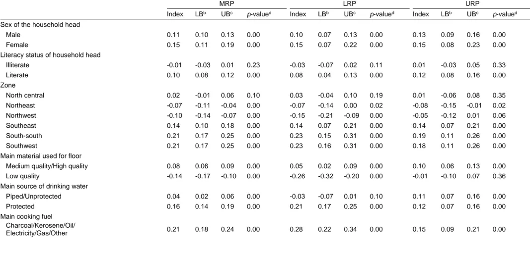
A similar conclusion can be drawn when looking at Table 7, which presents the set of relative polarization indices for each group defined by the covariates obtained by comparing their consumption distributions over time.13

If each of the group-specific polarization indices were close to 0, this would imply that after holding changes in the distributions of the covariates constant there is no residual polarization in consumption expenditures. The polarization we observe in the overall consumption distribution would then be due entirely to changing characteristics of the population over time. Instead, we see

13 _{Note that by comparing the sub-group distributions over time we are effectively controlling for the compositional}

13

a different scenario. Apart from the north central households and those with an illiterate head and no toilet facility, the estimates indicates a statistically significant increase of polarization in the sub-group distributions, except for households who reside in the northeast and northwest regions of the country and those with inadequate flooring in dwelling units, for whom some convergence toward the median is detected. The growth of polarization stems from a shift away from the median of both tails, and this seems to happen asymmetrically, as the LRP indices are in many cases more positive than the URPs—thus indicating more polarization in the lower than in the upper tail. Households headed by men, women or illiterates and households with good flooring material in dwellings, unsafe water and cooking with firewood, instead, are more polarized in the upper than in the lower tail of their consumption distribution—or at least they are so the same way. Overall, these patterns confirm that compositional shifts contributed little to the observed consumption polarization or, in other words, holding the changes in population characteristics constant does almost nothing to reduce overall polarization.14

The above conclusion suggests that the main drivers of polarization are to be found elsewhere, namely in the changes occurring over the decade in the consumption distributions of the groups defined by the covariates. While the covariate adjustment technique identifies the impact of changing population characteristics on the distribution of consumption expenditures, comparing the groups defined by the covariates directly makes it possible to analyse the changes within and between these groups’ consumption distributions. As already observed, many population sub-groups were both location-shifted (Tables 5 and 6) and more polarized (Table 7). To see what impact these location and shape shifts in the sub-groups’ distributions had on their relative positions within the overall consumption distribution, we compare the changes in deciles of the between-group relative distributions for 2003/04 and 2012/13 to the changes that would have occurred if only the medians or shapes of the groups had changed. More specifically, for each decile we decompose the absolute change:

(

:

) (

0 : 0

)

,

g C R −g C R ₍₁₁₎

into the marginal effect of the median shift from the 2003/04 relative density:

(

0L : 0L

) (

0: 0

)

,

g C R −g C R ₍₁₂₎

and those of the shape changes in the sub-groups’ consumption distributions:

(

0L :

) (

0L : 0L

)

,

g C R −g C R ₍₁₃₎

(

:

) (

0L :

)

,

g C R −g C R

(14) where g C R

(

:

)

and g C

(

0:R0

)

denote the relative density for comparison (C) to reference (R)

groups of the categorical variables in 2012/13 and 2003/04, respectively, whileR0 L and C0 L denote

14 _{This finding can also serve as a check of whether the observed changes in Nigerian consumption distribution are}

robust to sample size variations. That is, had the modifications in population characteristics been due to artefacts of the sample size, rather than to real population trends, our results would not be affected by them.

14

the distributions of the reference and comparison groups adjusted to have the same median as 2012/13 but with the same shape as 2003/04.1515 _{Summing up to the total difference given by}

Equation (11), these effects form a complete decomposition and allow us to determine what proportion of households were moved into or out of a decile of the overall distribution by changes in relative median- and group-specific shape.

The spatial distribution of household consumption expenditure definitely provided the most attractive results. Figure 6 presents the decomposition for each of the six Nigerian macro regions as compared to the rest of the country.

The solid bars show the total change by decile from Equation (11), and each of the lines represents one of the three components in the decomposition defined by Equations (12)-(14). We can see two ongoing distinctive patterns, both accentuating polarization. In the south-south and the southwest, relative to the rest of the country, residents tend to move out of the lower deciles of the distribution due to changes in the relative median. More precisely, had the location effect been the only one operating, we would have seen in both cases a clear transition of southeners from lower to upper deciles of the national distribution. However, the shape effect of both regions moved in the opposite direction, partially offsetting the positive impact of growth. Particularly in the lower deciles, the shape change is positive, indicating a clear trend of lower polarization in these areas that goes in the opposite direction vis-à-vis the national (residual) trend. This pattern is mirrored by what is going on in the upper deciles: a location effect higher than in the rest of the country (especially in the southwest) and an accentuated tendency to upper polarization in both regions. For what concerns the northeast and the northwest, the conflict-stricken areas, had the location effect been the only operating force we would have seen a disproportionate increase in people in these regions occupying the lower national deciles compared to the rest of the country— they basically lagged behind. The increase of polarization in the rest of the country helped to offset this effect, filling the lower deciles of households from other regions too, whereas for the rest of the distribution we observe in practice a generalized decline of the relative position of these regions in the national distribution. Finally, while the north central region improves relative to the rest of the country in lower deciles, the southeast region comes to show a more articulated pattern of distributional change.

Results for the other covariates (not shown here but available upon request) looked as expected: compared to 2003/04, households with an illiterate head or not having good cooking material, toilet, floor and safe water were all increasingly occupying the lower deciles of the distribution, and the gap in terms of consumption with the rest was increasing. Instead, the relative fraction of households headed by females in the upper deciles of the distribution was rising during the period, whereas male-headed households were moving into the deciles below the median. In spite of the fact that Nigerian society is mainly patriarchal, where men have better access to productive resources than women, poverty seems greater among men than women.

15 _{The decomposition follows the spirit of that presented in Bernhardt et al. (1995) and Handcock and Morris (1998,}

15

5 Concluding remarks

In the last two decades there have been two emerging narratives on Sub-Saharan Africa. The first paints a picture of an emerging continent where the middle classes are expanding, and prosperity is reaching large swaths of the population (African Development Bank 2011; Fine et al. 2012). The other narrative acknowledges the relatively robust growth in the past two decades, but points to slow reduction in poverty. According to this second narrative, the lack of faster reduction in poverty may be due, in part, to increasing disparities.

Nigeria, the most populous country in the African continent, experienced a stable and sustained growth over recent years but, despite this, the outcomes in terms of poverty reduction have not been satisfactory: while poverty seems to have declined in the coastal south and around the federal capital, Abuja, a large belt of northeastern states have experienced a clear stagnation in poverty reduction.

Our conjecture is that Nigeria in the last decade has also gone through significant changes in the distribution of economic resources that generated mainly, but not exclusively, a fast rise in inequalities. Inequality, we argue, represents just one aspect of the whole problem: the country is undergoing through a fast process of polarization. Polarization is increasingly becoming a concern in many developing countries. In income-polarized societies people cluster around group means and tend to be far from the mean/median of the overall distribution; as a consequence, the middle class in polarized societies struggles to consolidate its position. This has several economic consequences for the country, but also reflects in growing political instability.

Studies on polarization in Nigeria are surprisingly few and have tackled the topic with a narrow approach. This paper aims at filling this gap by undertaking an analysis that is innovative from different points of view. First, the period considered is a decade; the length of the time span, in absence of big shocks, is crucial if one wants to detect significant transformations in the welfare distribution. Second, the welfare measures compared (consumption per capita) are fully homogeneous. To obtain this we made use of survey-to-survey estimation techniques (Elbers et al. 2003) and tested their robustness using different methodologies and comparing results.

Finally, and most importantly, we employed the ‘relative distribution’ approach (Handcock and Morris 1998, 1999) to analyse changes in the Nigerian household consumption distribution in the period considered. The novelty of this method consists in providing a non-parametric framework for taking into account all of the distributional differences that could arise in the comparison of distributions over time and space. In this way, we have been able to summarize multiple features of the expenditure distribution that would not be detected easily from a comparison of standard measures of inequality and polarization.

The analysis reveals significant changes in the consumption distribution. Net of an average increase in consumption, a clear rise in polarization is detected, meaning that the distributional movements observed between 2003/04 and 2012/13 hollowed out the middle of the Nigerian household consumption distribution and increased concentration of the mass toward the highest and lowest deciles.

This pattern of distributional change, however, is not entirely homogeneous within the country, but varies from zone to zone. By means of covariates analysis, controlling by spatial characteristics of household head, we are able to highlight a relevant issue: in the south (southwest and

south-16

south) relative to the rest of the country lower deciles tend to be emptied accentuating the tendency to upper polarization in both regions. In the northwest and in the conflict-stricken northeast regions, had the growth effect been the only operating force, we would have seen a disproportionate increase in people of this region occupying the lower national deciles compared to the rest of the country.

These modifications occurred between 2003/04 and 2012/13 and describe a situation of accentuated polarization where households living in the north increasingly moved from the centre towards the bottom of the consumption distribution, while southern households increasingly moved upward. The overall impact was a generalized hollowing out of the distribution centre and a further accentuation of the north-south divide already characterizing the country.

Understanding the political and economic consequences of these sharp distributional changes is beyond the scope of this paper. However, some clear trends can already be foreseen. As mentioned, the non-consolidation of the middle class is the first and more obvious side effect of accentuated polarization. Second, and not so much explored in the context of developing countries, is the tendency of polarized society to be more conflict-prone. Recent episodes in Brazil, Egypt and Turkey suggest the existence of this link between polarization and conflict, yet so far no relevant empirical evidence has been produced to underpin the existing theoretical models (Esteban and Ray 1999, 2008, 2011). Nigeria is clearly an ideal candidate for such analysis, and our future research will be directed toward understanding how existing conflicts in Nigerian societies can be interpreted and linked to the patterns of polarization.

References

African Development Bank (2011). Annual Report. Tunis: Statistics Department of the African Development Bank Group.

Ahmed, F.C., C. Dorji, S. Takamatsu, and N. Yoshida (2014). ‘Hybrid Survey to Improve the Reliability of Poverty Statistics in a Cost-Effective Manner’. Policy Research Working Paper 6909. Washington, DC: World Bank.

Aigbokhan, B.E. (2000). ‘Poverty, Growth and Inequality in Nigeria: A Case Study’. AERC Research Paper 102. Nairobi: African Economic Research Consortium.

Araar, A. (2008). ‘On the Decomposition of Polarization Indices: Illustrations with Chinese and Nigerian Household Surveys’. Working Paper 08-06. Montréal: Centre Interuniversitaire sur le Risque, les Politiques Économiques et l’Emploi (CIRPÉE).

Araar, A., and J.-Y. Duclos (2013). User Manual for Stata Package DASP: Version 2.3. PEP, World

Bank, UNDP and Université Laval. Available at

http://dasp.ecn.ulaval.ca/modules/DASP_V2.3/DASP_MANUAL_V2.3.pdf (accessed 27 October 2014).

Awoyemi, T.T., and A. Araar (2009). ‘Explaining Polarization and its Dimensions in Nigeria: A DER Decomposition Approach’. Paper prepared for the 14th Annual Conference on ‘Econometric Modelling for Africa’, Abuja, Nigeria, 8-10 July 2009.

Awoyemi, T.T., I.B. Oluwatayo, and A. Oluwakemi (2010). ‘Inequality, Polarization and Poverty in Nigeria’. Working Paper 2010-04. Nairobi: Partnership for Economic Policy (PEP).

17

Beegle, K., J. De Weerdt, J. Friedman, and J. Gibson (2010). ‘Methods of Household Consumption Measurement through Surveys: Experimental Results from Tanzania’. Policy Research Working Paper 5501. Washington, DC: World Bank.

Bernhardt, A., M. Morris, and M.S. Handcock (1995). ‘Women’s Gains or Mens Losses? A Closer Look at the Shrinking Gender Gap in Earnings’. American Journal of Sociology, 101: 302-28. Birdsall, N. (2010). ‘The (Indispensable) Middle Class in Developing Countries; Or, the Rich and

the Rest, Not the Poor and the Rest’. Working Paper 207. Washington, DC: Center for Global Development.

Clementi, F., A.L. Dabalen, V. Molini, and F. Schettino (2014). ‘Economic Polarization: The Dark Side of Nigeria’. Paper presented at the IfW Centenary Conference ‘Fair and Sustainable Prosperity in the Global Economy’, Kiel, Germany, 13-14 June 2014.

Deaton, A., and M. Grosh (2000). ‘Consumption’. In M. Grosh, and P. Glewwe (eds), Designing

Household Survey Questionnaires for Developing Countries: Lessons from 15 Years of the Living Standards Measurement Study. Oxford: Oxford University Press.

Duclos, J.-Y., J.-M. Esteban, and D. Ray (2004). ‘Polarization: Concepts, Measurement, Estimation’. Econometrica, 72: 1737-72.

Easterly, W. (2001). ‘The Middle Class Consensus and Economic Development’. Journal of Economic

Growth, 6: 317-35.

Elbers, C., J.O. Lanjouw, and P. Lanjouw (2003). ‘Micro-Level Estimation of Poverty and Inequality’. Econometrica, 71: 355-64.

Esteban, J.-M., and D. Ray (1999). ‘Conflict and Distribution’. Journal of Economic Theory, 87: 379-415.

Esteban, J.-M., and D. Ray (2008). ‘Polarization, Fractionalization and Conflict’. Journal of Peace

Research, 45: 163-82.

Esteban, J.-M., and D. Ray (2011). ‘Linking Conflict to Inequality and Polarization’. The American

Economic Review, 101: 1345-74.

Ferreira, F.H.G., J. Gignoux, and M. Aran (2011). ‘Measuring Inequality of Opportunity with Imperfect Data: The Case of Turkey’. Journal of Economic Inequality, 9: 651-80.

Fine, D., A. van Wamelen, S. Lund, A. Cabral, M. Taoufiki, N. Dörr, A. Leke, C. Roxburgh, J. Schubert, and P. Cook (2012). ‘Africa at Work: Job Creation and Inclusive Growth’. Washington, DC: McKinsey Global Institute.

Fortin, N., T. Lemieux, and S. Firpo (2011). ‘Decomposition Methods in Economics’. In O. Ashenfelter, and D. Card (eds), Handbook of Labor Economics. North Holland: Elsevier.

Foster, J.E., and M.C. Wolfson (1992). ‘Polarization and the Decline of the Middle Class: Canada and the US’. OPHI Working Paper 31. Oxford: University of Oxford. [Now in Journal of

Economic Inequality, 8: 247-73].

Handcock, M.S. (2014). ‘Relative Distribution Methods’. Los Angeles, CA. Version 1.6-3. Project home page at www.stat.ucla.edu/~handcock/RelDist (accessed 27 October 2014).

Handcock, M.S., and M. Morris (1998). ‘Relative Distribution Methods’. Sociological Methodology, 28: 53-97.

18

Handcock, M.S., and M. Morris (1999). Relative Distribution Methods in the Social Sciences. New York: Springer-Verlag Inc.

Hao, L., and D.Q. Naiman (2010). Assessing Inequality. Thousand Oaks, CA: SAGE Publications. Jenkins, S.P., and P. Van Kerm (2005). ‘Accounting for Income Distribution Trends: A Density

Function Decomposition Approach’. Journal of Economic Inequality, 3: 43-61.

Morris, M., A.D. Bernhardt, and M.S. Handcock (1994). ‘Economic Inequality: New Methods for New Trends’. American Sociological Review, 59: 205-19.

Ogunyemi, O.I. (2013). ‘Gender, Market Participation and Income Polarisation among Farming and Non-Farming Households in Nigeria’. Paper presented at the World Bank Workshop on ’African Agriculture: Myths and Facts’, Washington, DC, 20-22 November 2013.

Ogunyemi, O.I., and O.A. Oni (2011). ‘Income Bipolarization and Poverty: Evidence from Rural Nigeria’. Journal of American Science, 7: 722-31.

Ogunyemi, O.I., O.A. Oni, T.T. Awoyemi, and S.A. Yusuf (2011). ‘Income Polarization and Bipolarization across Rural Households’ Socio-Economic Features in Nigeria’. World Rural

Observations, 3: 62-72.

Pressman, S. (2007). ‘The Decline of the Middle Class: An International Perspective’. Journal of

Economic Issues, 41: 181-200.

Stifel, D., and L. Christiaensen (2007). ‘Tracking Poverty over Time in the Absence of Comparable Consumption Data’. World Bank Economic Review, 21: 317-41.

Tarozzi, A. (2007). ‘Calculating Comparable Statistics from Incomparable Surveys, with an Application to Poverty in India’. Journal of Business & Economic Statistics, 25: 314-36.

Van Kerm, P. (2003). ‘Adaptive Kernel Density Estimation’. The Stata Journal, 3: 148-56. Wolfson, M.C. (1994). ‘When Inequalities Diverge’. The American Economic Review, 84: 353-58. World Bank (2013). ‘Nigeria. Where Has All the Growth Gone? A Poverty Update’. Washington,

19 Table 1: Regression results of POV_MAP imputation model

Dependent variable: log of consumption per capita in 2010 Naira spatially deflated

Explanatory variablea _Coefficientb _t-statistic

Number of people in household -0.06 *** -7.23 Population age less than 15 years and population aged over 64 years -0.03 *** -4.07 Children between 0 and 4 years old -0.07 *** -3.56

Adult females -0.02 -1.52

Number of females 65 years and above -0.03 -1.36 Age of household head 0.00 -0.22 Age of household head squared 0.00 -1.37 Marital status of household head 0.07 *** 7.10 Marital status of household head is polygamous marriage 0.03 0.67 Sex of household head 0.04 0.96 Number of years of education for household head 0.01 *** 6.96

Literacy status of household head 0.09 ** 2.37

Self-employed in non-agricultural sector 0.05 *** 3.08 Sector of activity by broad group of household head -0.04 -0.93 Ownership of dwelling unit 0.12 *** 3.72 Area of residence (in square meters) 0.08 *** 4.82 Ownership of radio 0.06 *** 4.98 Ownership of television 0.08 *** 4.34 Ownership of refrigerator 0.07 *** 3.62 Ownership of motorcycle 0.02 0.66 Ownership of sewing machine -0.01 -0.33

Ownership of stove 0.00 -0.01 Ownership of bicycle 0.14 ** 2.02 Ownership of car 0.25 *** 6.39 Ownership of generator 0.12 *** 3.36 Ownership of iron 0.02 0.64 Ownership of fan -0.03 -0.88

Ownership of bed or mattress 0.01 0.21 Main material used for floor - Low quality -0.06 *** -3.12 Main material used for floor - Medium quality -0.08 *** -4.91 Main source of drinking water - Protected 0.07 1.62 Main source of drinking water - Unprotected 0.12 ** 2.56

Main cooking fuel - Firewood -0.22 *** -4.11

Main cooking fuel - Kerosene/Oil -0.10 * -1.88

Main cooking fuel - Other -0.18 *** -2.86

Main toilet facility - No facility -0.01 -0.24

Main toilet facility - Flush toilet 0.07 * 1.95 Garbage and trash disposal -0.01 * -1.92

_cons 11.58 *** 92.23

2

R 0.46

Notes: (a) state level dummies (Lagos state omitted) and zone interacted variables (southwest zone omitted) not reported; (b) *** p<0.01, ** p<0.05, * p<0.10.

20

Table 2: Mean and standard deviation of relative polarization indices over R =50 simulation runs for three alternative imputation techniques MRPa _LRPb _URPc POV_MAPd Mean 0.13 0.12 0.13 Standard deviation 0.00 0.01 0.01 MI_REGe Mean 0.11 0.14 0.09 Standard deviation 0.01 0.02 0.01 MI_PMMf Mean 0.11 0.11 0.11 Standard deviation 0.01 0.02 0.01

Notes: (a) MRP = median relative polarization index; (b) LRP = lower relative polarization index; (c) URP = upper relative polarization index; (d) POV_MAP = multiple imputation method using Equation (1); (e) MI_REG = Gaussian normal regression imputation method; (f) MI_PMM = predictive mean matching imputation method.

21

Table 3: Summary measures of Nigerian household total consumption expenditure per capita

2003/04 2012/13 Mean 84,874 99,084 Median 71,168 76,193 Standard deviation 58,707 122,250 Skewness 2.48 39.32 Kurtosis 15.55 2,818.97 Consumption shares Bottom 5% 1.05 0.93 Bottom 10% 2.64 2.29 Bottom 20% 6.90 5.97 Top 20% 41.14 45.45 Top 10% 25.43 29.52 Top 5% 15.35 18.97 Inequality measures Gini 0.34 0.39 Theil 0.20 0.29 Polarization measuresa Foster-Wolfson 0.30 0.35 Duclos-Esteban-Ray 0.21 0.24

Notes: (a) the Duclos-Esteban-Ray index has been computed with the polarization sensitivity parameter α set at 0.5. Source: Authors’ calculation based on 2012/13 GHS panel data and imputed 2003/04 NLSS data.

22 Table 4: Relative polarization indicesa

Index Value LBb _UBc _p-valued

MRP 0.12 0.11 0.13 0.00

LRP 0.11 0.08 0.14 0.00

URP 0.13 0.10 0.16 0.00

Notes: (a) MRP = median relative polarization index, LRP = lower relative polarization index, URP = upper relative polarization index; (b) lower bound of the 95 per cent confidence interval; (c) upper bound of the 95 per cent confidence interval; (d) refers to the null hypothesis of no change with respect to the reference distribution, i.e. that the index equals 0.

23

Table 5: Summary measures for Nigerian household consumption expenditure by population subgroups, 2003/04 and 2012/13

2003/04 2012/13

Mean Median Pop. share Cons. share Gini Theil Mean Median Pop. share Cons. share Gini Theil

Sex of the household head

Male 83,692 69,897 0.90 0.88 0.34 0.20 97,125 74,340 0.90 0.88 0.39 0.29

Female 95,049 81,550 0.10 0.12 0.32 0.18 116,276 90,664 0.10 0.12 0.39 0.29

Literacy status of household head

Illiterate 76,980 65,113 0.64 0.58 0.33 0.19 76,391 60,686 0.34 0.26 0.38 0.33 Literate 98,741 83,335 0.36 0.42 0.34 0.19 110,838 86,203 0.66 0.74 0.38 0.26 Zone North central 79,120 67,318 0.14 0.13 0.34 0.19 86,507 74,273 0.14 0.12 0.33 0.18 Northeast 86,745 74,290 0.12 0.13 0.33 0.18 78,168 65,903 0.14 0.11 0.35 0.22 Northwest 72,003 59,182 0.25 0.21 0.35 0.21 70,037 53,134 0.25 0.18 0.38 0.40 Southeast 93,147 74,442 0.12 0.13 0.37 0.23 111,485 80,006 0.12 0.13 0.43 0.33 South-south 85,468 70,298 0.17 0.17 0.34 0.19 114,467 87,784 0.15 0.18 0.38 0.25 Southwest 98,279 86,632 0.20 0.23 0.30 0.15 140,493 118,426 0.20 0.28 0.32 0.19

Main material used for floor

Medium quality/High quality 94,154 79,889 0.61 0.67 0.33 0.19 103,085 80,192 0.91 0.95 0.39 0.29

Low quality 70,616 59,955 0.39 0.33 0.33 0.18 58,794 45,057 0.09 0.05 0.36 0.24

Main source of drinking water

Piped/Unprotected 84,337 71,298 0.62 0.62 0.34 0.19 94,766 70,509 0.46 0.44 0.39 0.32

Protected 85,761 71,025 0.38 0.38 0.35 0.20 102,709 81,482 0.54 0.56 0.39 0.27

Main cooking fuel

Charcoal/Kerosene/Oil/

Electricity/Gas/Other 112,935 94,852 0.25 0.34 0.32 0.17 157,614 129,633 0.26 0.41 0.34 0.21

Firewood 75,369 64,282 0.75 0.66 0.33 0.18 78,857 64,111 0.74 0.59 0.36 0.26

Main toilet facility

Flush toilet/Improved pit latrine/Uncovered pit latrine/Other

86,957 72,732 0.83 0.85 0.34 0.20 105,467 81,057 0.78 0.83 0.40 0.30

No facility 74,782 64,066 0.17 0.15 0.32 0.17 75,919 63,770 0.22 0.17 0.34 0.20