DOTTORATO DI RICERCA IN MATEMATICA
XVI CICLO
Silvia Rensi
Analyzing complex choices
through generalized spectral
analysis: preference formation.
Relatore
This Thesis deals principally with an application of the so–called generalized spectral analysis to a problem of economic science: preference formation. The needed mathematical framework is based on group representation theo-ry, isotypic projections, spectral analysis on group.
The basic purpose of the whole is essentially efficient data analysis; this is obtained through the application of generalized spectral analysis (a genera-lization of classical spectral analysis, the one used in time series analysis, for example) to group theory . This kind of approach is very strong and allows to detect in data particular effects which are not appreciable from a direct analysis of data.
Our work is modeled on some recent results of M. E. Orrison and B. L. Law-son who applied generalized spectral analysis to political science; their work provides a sistematic way to detect influential coalitions in a political voting process.
In Chapter 1 we recall some mathematical background in order to reach a deeper comprehension of spectral analysis and its applications. The content of the chapter develops through some basic notion on group representation theory, a brief account on the representation theory of the symmetric group, the concept of Fourier transform and the techniques of the Fast Fourier trans-form and finally spectral analysis and its applications.
Section 1.1 is given up to a brief account on group representation theory; it is nothing else that a recall of the concept of representations, characters, irreducible representations and so on.
can be decomposed in what is the so–called isotypic decomposition.
In section 1.3 we recall briefly the construction of all irreducible represen-tations of the symmetric group and the decomposition of the permutation module.
Section 1.4 is given up to Fourier transform on groups. Originally discovered by Gauss and later made famous by Cooley and Tukey, the Fast Fourier trans-form may be viewed as an algorithm which efficiently computes the Fourier Transform. Recently, there has developed a growing literature related to the construction of algorithms which generalize the FFT from the point of view of the theory of group representations. These sort of generalizations are “natural” as mathematical constructs, but in point of fact they too have been motivated by applications, such as, as in our context, efficient data analysis.
Section 1.5 is the core of Chapter 1 and provides an account on generali-zed spectral analysis. Spectral analysis is a non–model based approach to data analysis, formulated in general group theoretic setting by Diaconis; it extends the classical spectral analysis of time series. The idea of spectral analysis is that often data has natural symmetries, encapsulated in the exi-stence of a symmetry group for the domain of the data. The organizing principle of spectral analysis is the understanding of data trough its decom-position according to these symmetries.
If X is a finite set, G a group acting on X and L(X) the vector space of complex–valued functions on G, then L(X) may be decomposed as an or-thogonal direct sum of G-invariant subspaces
L(X) = V1⊕ · · · ⊕ Vh,
called the isotypic decomposition. Spectral analysis takes the form of com-puting the projections of the data onto these subspaces and judging which projections are significant. The use of generalized FFTs for spectral analysis is the efficient computation of the projections.
Of particular interest is the analysis of ranking problems. Data sometimes come in the form of rank of preferences. Most anyone who analyzes such data looks at simple averages, such as the proportion of times each item was ranked first and the average rank for each item. There are first order
on the number of times items i and j are ranked in position k and l. Similarly there are third and higher order statistics of various type.
Diaconis underlines the crucial point od spectral analysis: “a basic idea of data analysis is this: if you’ve found some structure, take it out and look at what is left. Thus, to look at second order statistic it is natural to substract away the observed first order structure. This leads to a natural decomposition of the original data into orthogonal pieces”.
Chapter 2 is given up to the exposition of some recent works of M. E. Orri-son and B. L. LawOrri-son (see [22], [23] and [24]) on noncommutative harmonic analysis applied to political voting.
Diaconis extended the classical spectral analysis of time series to a non–time series subject, for the analysis of discrete data which has a noncommutative structure. New efforts have been made in order to apply spectral analysis to a non–time series subject in political science, above all in the analysis of voting. Spectral analysis has been already used in political science to identify cycles in time series data.
Orrison and Lawson introduced a generalization of spectral analysis as a new instrument for political scientist; they used the powerful machinery of spectral analysis to analyze political voting data. In particular, they analyzed votes of the nine judges of the United States Supreme Court and detected influential coalitions. With this theory political scientist can use spectral analysis as a method for identifying substantively important dynamics in politics, rather then just as a diagnostic tool.
The idea followed by Orrison and Lawson is to consider political voting data as elements of a mathematical framework; then the features of that framework can be used to work out natural interpretations of the data. The mathema-tical framework corresponding to voting data has many components, each of which encapsulates information on particular coalition effects; the decompo-sition of data with respect to these components provides the identification of influential coalitions.
application of generalized spectral analysis to preference formation.
Our context can be summarized as follows. We interpret the decision to vote for a party as a process of delegation to decision makers having a simplified system of preferences. Each person in a population votes for the political party that place priority on one or more issues that they consider important. On the basis of a survey on preferences of population, we have simulated a delegation procedure which chart the selection process of a particular party. Making use of noncommutative harmonic analysis, we decomposed the dele-gation function and isolated the effect of a particular affinity, or a combination of either the pair of items that characterize a party.
To be more precise, our construction bases itself on these considerations. Individuals facing a choice are often not able to make a full comparison bet-ween alternatives. Even if they are able to pin down their preferences for certain characteristics of an object (for instance, a car), they would proba-bly be able to compare only a few of them. In the case of a car, one person would take into account room and safety, while somebody else’s order ranking would be based on speed and acceleration. We can interpret this evaluation imagining that our “complete” selves delegate choices to a sort of simplified self.
In public choice theory, political parties present themselves as decision ma-kers committed to following a given preference order when faced with future choices. Parties collect delegations from people having similar preferences. Traditionally parties have a complete system of preferences and they collect a delegation from the people having an order of preferences “not far” from the one expressed by the party.
Here instead of following this traditional path, we adopt a similar approach to the one presented in “car choice”. We describe parties as simplified systems of preferences and the process of delegation as giving the power of choice to parties that correspond to this simplified prefe-rence order.
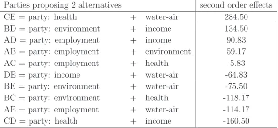
to which they attach more importance, it could be that the items chosen complement themselves well, being able to attract a large share of voters, or alternatively the two items could reciprocally depress their power of attrac-tion. When facing a simplified set of options, the right combination could be of fundamental importance.
I would like to thank my advisor, prof. Andrea Caranti, who introduced me to the variegated world of the subject of this Thesis.
I would like to give my heartfelt thanks to prof. Enrico Zaninotto, who helped me for almost all the period of my work and has been supportive and helpful through various difficult times.
Preface iii
Acknowledgements ix
1 Spectral analysis and group representation theory 1
1.1 Representation theory . . . 2
1.2 Isotypic projections . . . 3
1.3 Representations of the symmetric group . . . 7
1.3.1 Tableaux, tabloids and Young subgroups . . . 7
1.3.2 Specht modules . . . 10
1.3.3 The decomposition of Mλ . . . 12
1.4 Fourier transform on groups . . . 16
1.4.1 Fourier transform on the symmetric group . . . 18
1.5 Spectral analysis on groups . . . 20
1.5.1 Time series analysis . . . 21
Example 1: Time series analysis. . . 21
1.5.2 Spectral analysis of full and partially ranked data . . . 22
Example 2: Full rankings. . . 23
Example 3: Full rankings (again). . . 26
1.5.3 General considerations . . . 29
Example 4: Partial rankings. . . 30
2 Spectral analysis and voting 35 2.1 Noncommutative harmonic analysis of voting in committees . 35 2.2 Coalitions . . . 37
2.3 A five people committee . . . 38
2.3.1 One person in the minority. . . 39
2.4 Analysis of the Supreme Court . . . 43
3 Spectral analysis and preference formation 45 3.1 Introduction . . . 46
3.2 Individual preferences, parties and public choice . . . 47
3.3 Voting for incomplete parties and the power of combination . 51 3.4 Detecting the power of combination . . . 52
3.4.1 Preferences combination . . . 52
3.5 An application to a survey . . . 54
3.5.1 Transitivity of preferences . . . 55
Total orders . . . 56
Consistent preference systems . . . 59
3.5.2 Generalized spectral analysis . . . 61
First order effects . . . 63
Second order effects . . . 64
Interpretation: Mallow’s method . . . 65
Significance . . . 68
3.6 Conclusions . . . 69
1
Spectral analysis and group
representation theory
As explained in the Preface and examined carefully in Chapter 3, our work want to be an application of the so–called generalized spectral analysis in the field of economic science.
Spectral analysis is a non–model based approach to data analysis, formu-lated in general group theoretic setting by Diaconis (see [9], [10]); it extends the classical spectral analysis of time series. The idea of spectral analysis is that often data has natural symmetries, encapsulated in the existence of a symmetry group for the domain of the data. The organizing principle of spectral analysis is the understanding of data trough its decomposition ac-cording to these symmetries.
In order to reach a deeper comprehension of spectral analysis and its ap-plications, we need some theoretical backgrounds. In this Chapter first of all we will recall some basic notation and terminology of group representation theory. It will follow a brief account on the representation theory of the sym-metric group: we need the construction of all irreducible representations of
Sn and the decomposition of the permutation module. In our exposition it
will be of great importance the concept of Fourier transform and the tech-niques of the Fast Fourier Transform. The core of the chapter will be spectral analysis and its applications.
1.1
Representation theory
We recall some general terminology and notation about group representation theory that will be useful in the following. Representation theory can be couched in terms of matrices or in the language of modules; we will occasio-nally consider both approaches. We will follow Serre (see [42]).
Let G be a finite group and V a finite dimensional vector space over C. Let GL(V ) be the group of automorphisms of V . A representation of G is a group homomorphism ρ : G −→ GL(V ). If the homomorphism ρ is under-stood, then we also say that V is a representation of G. In the language of modules, V is also called a G–module. We call dρ := dim V the degree of
the representation ρ.
Two representations ρ1 and ρ2 of a group G on V1 and V2 are said to
be isomorphic if there exists an isomorphism T : V1 −→ V2 such that
ρ1(s) = T−1◦ ρ2(s) ◦ T , for all s ∈ G. In other words, in matrices language,
two representations are isomorphic if they differ only by a change of basis, i.e. there exists an invertible matrix A such that ρ1(s) = A−1ρ2(s)A.
The character of ρ is the function χ : G −→ C where χ(s) is the usual trace of ρ(s). Note that the character of a representation of G is constant on the conjugacy classes of G.
A subspace W of V is invariant if ρ(s)(w) ∈ W , for all s ∈ G, w ∈ W . A representation is said to be irreducible if it contains no non–trivial in-variant subspaces. If C1, . . . , Ch are the distinct conjugacy classes of G, then
there are h distinct irreducible representations W1, . . . , Wh of G (up to
iso-morphisms). Irreducible representations are the fundamental blocks of all representations of a finite group. More precisely, any representation is iso-morphic to a direct sum of irreducible representations.
1.2
Isotypic projections
As we will see, spectral analysis applied to group representation theory is strongly based on the fact that any representation of a finite group can be decomposed in what is the so–called isotypic decomposition. Serre (see [42]) gives a complete description of the decomposition, while Diaconis and Rock-more (see [12]) and Maslen, Orrison and RockRock-more (see [29]) provide efficient algorithms for the computation of isotypic projections.
Let G be a finite group and X = {x1, . . . xn} a finite set. Suppose that
G acts transitively on X; X is called a homogeneous space for G. Let L(X) denote the vector space of all complex-valued functions on X. Then L(X) naturally admits a representation ρ of G defined by
ρ : G −→ GL(L(X)) ρ(s) = ρs
where
ρs : L(X) −→ L(X)
ρs(f )(x) = f (s−1x)
for each s ∈ G, x ∈ X and f ∈ L(X).
The vector space L(X) has a natural basis {δx}x∈X, where
δx(x′) =
½ 1 if x = x′
0 otherwise.
We will refer to {δx}x∈X as the delta basis of L(X). Note that dim L(X) =
|X| := dX. By choosing a basis for L(X), we may identify each linear
trans-formation on L(X) with a dX × dX matrix. Thus, we will assume that each
linear transformation on L(X) is written as a matrix with respect to the delta basis of L(X). In particular, if s ∈ G, then ρs corresponds to a dX× dX
matrix with one 1 in each row and column and zeros elsewhere.
The representation ρ obtained by L(X) is a permutation representation of G. We recall the following
DEFINITION 1.2.1 Let G be a finite group acting on a finite set X and V a vector space with a basis {ex}x∈X indicized by the elements of X. The
per-mutation representation associated to X is the representation ϕ defined by ϕ : G −→ GL(V ), ϕ(s) = ϕs, where
ϕs: V −→ V
ϕs(ex) = esx
for each s ∈ G and x ∈ X.
Now, ρs(δx) : X −→ C x′ 7→ δx(s−1x′) but δx(s−1x′) = ½ 1 if x = s−1x′ 0 otherwise = ½ 1 if sx = x′ 0 otherwise = ρsx(x ′),
which shows indeed that ρ is a permutation representation of G.
We recall that, if X = {x1, . . . , xn} is a finite set, for any xi ∈ X, Stab(xi)
denote the stabilizer of xi in G, that is the subgroup of elements of G which
fix xi. The representation ρ of G naturally defined by L(X) is precisely the
permutation representation of G on the quotient space G/ Stab(xi), for any
i. Equivalently, it is the representation obtained by inducing the trivial rep-resentation from Stab(xi) to G.
As a representation space for G, L(X) has a basis indipendent decompo-sition into G-invariant subspaces, known as isotypic subspaces. Following Serre (see [42]), the so–called isotypic decomposition of L(X) may be ex-plained as follows.
Let ρ1, . . . , ρh be a complete set of non-isomorphic irreducible
representation space for G, so can be decomposed into a direct sum of irre-ducible G-invariant subspaces. That is
L(X) =
m
M
j=1
Uj.
where ρ(s)Uj = Uj, for each Uj 6= 0, and no trivial subspace of Uj has this
property. For each j = 1, . . . , m, ρ(s) restricted to Uj gives an irreducible
representation of G. In this decomposition of L(X) there will be isomorphic copies of Uj, so we can define Vi as the subspace of L(X) given by the
direct sum over all Uj which define representations isomorphic to ρi, for each
i = 1, . . . , h. So the isotypic decomposition of L(X) is
L(X) =
h
M
i=1
Vi, (1.1)
where Vi is called the i-isotypic subspace of ρ. (Note that some of the Vi
may be zero).
Given an arbitrary f ∈ L(X), we may compute the projection of f onto each isotypic subspace of L(X). So, if f ∈ L(X), f may be written uniquely as
f = f1+ · · · + fh, (1.2)
where fi is called the isotypic projection of f onto the isotypic subspace
Vi.
There is a classical theorem which allows to calculate the projection of a group representation V onto its isotypic subspaces (Serre [42], theorem no. 8, pag. 21).
THEOREM 1.2.1 (see Serre, [42]) Let G be a finite group and ϕ : G −→ GL(V ) a representation of G. Let ϕ1, . . . , ϕh be a complete set of
non-isomorphic irreducible representations of G and σ1, . . . , σh the corresponding
each i = 1, . . . , h, define pi as the projection of V on Vi. Then pi = deg(ϕi) |G| X s∈G σi(s)ϕ(s) (1.3)
for each i = 1, . . . , h, where σi(s) is the conjugate of σi(s).
In our particular case, where the representation is the permutation represen-tation ρ obtained by L(X), more can be said.
THEOREM 1.2.2 Let G be a finite group acting on a finite set X. Let ρ be the associated permutation representation of G in L(X), let ρ1, . . . , ρh
be a complete set of non-isomorphic irreducible representations of G and χ1, . . . , χh the corresponding characters.
For each f ∈ L(X), let f1+ · · · + fh be the isotypic decomposition of f .
Then fi(x) = deg(ρi) |G| X s∈G χi(s)f (sx) (1.4)
for each x ∈ X and i = 1, . . . , h.
Proof. We calculate fi(x) = pi(f (x)) = = deg(ρi) |G| X s∈G χi(s) (ρ(s)f ) (x) = = deg(ρi) |G| X s∈G χi(s)f (s−1x) = = deg(ρi) |G| X s∈G χi(s−1)f (s−1x) = = deg(ρi) |G| X g∈G χi(g)f (gx).
where we used the elementary property χi(s) = χi(s−1).
1.3
Representations of the symmetric group
In this section we recall briefly the construction of all irreducible representa-tions of the symmetric group Sn. Sagan (see [41]) gives a very nice exposition
of the construction and James (see [18]) and James and Kerber (see [19]) pro-vides an encyclopedic account with many references.
We know that the number of irreducible representations of Sn is equal to the
number of conjugacy classes of Sn(see Serre [42]), which is also the number of
partions of n. It is not obvious how to associate an irreducible representation of Sn with each partition λ = (λ1, . . . , λk) of n, but is quite easy to find a
corresponding group Sλthat is an isomorphic copy of Sλ1×Sλ2×· · · Sλk inside
Sn. The right number of irreducible representations of Sn may be produced
by inducing the trivial representation on each Sλ up to Sn.
1.3.1
Tableaux, tabloids and Young subgroups
Let λ ⊢ n be a partition of n; this means that λ = (λ1, . . . , λk)
with λ1 ≥ · · · ≥ λk> 0 and λ1+ · · · + λk = n. In this case k = h(λ) is called
the length of λ. We can visualize λ as follows.
DEFINITION 1.3.1 Let λ = (λ1, . . . , λk) ⊢ n be a partition of n. A
Young diagram of shape λ is a left-justified array of square boxes with λi
boxes in row i, with 1 ≤ i ≤ k.
DEFINITION 1.3.2 A Young tableau t of shape λ is a Young diagram of shape λ with integers 1, . . . , n placed without repetition in its boxes. For example, a Young tableau of shape (4, 3, 1, 1) is
t =
3 1 2 4 5 6 8 7 9
Obviously there are n! tableaux of a fixed shape.
DEFINITION 1.3.3 Two Young tableaux t1 and t2 of shape λ are said to
be equivalent if they differ only by permuting the entries within a given row. An equivalence class of Young tableaux of a fixed shape is called a tabloid of the same shape.
For example, two equivalent Young tableaux of shape (4, 3, 1, 1) are
t1 = 1 2 3 4 5 6 7 8 9 , t2 = 2 1 3 4 7 5 6 8 9 .
We may think of a tabloid as a tableau with unordered row entries. A given tabloid is denoted by forming the representative Young tableau and removing the internal vertical lines. For example, the tabloid of shape (4, 3, 1, 1)
{t} = 9 8 5 1 6 7 2 3 4
represents the equivalence class of the t1 and t2 of the previous example.
If λ = (λ1, . . . , λk) ⊢ n, then the number of tableaux in any given equivalence
Now we wish to associate with a partition λ a subgroup of Sn.
DEFINITION 1.3.4 Let λ = (λ1, . . . , λk) ⊢ n be a partition of n. The
Young subgroup of Sn corresponding to λ is
Sλ = S{1,2,...,λ1}× S{λ1+1,λ1+2,...,λ1+λ2}× · · · × S{n−λk+1,n−λk+2,...,n}
where S{i,j,...,l} means the subgroup of Sn permuting only the integers in the
brackets.
These subgroups are named in honor of the Reverend Alfred Young, who was among the first to construct the irreducible representations of Sn. For
example,
S(3,3,2,1)= S{1,2,3}× S{4,5,6}× S{7,8}× S{9}
∼= S3× S3× S2× S1.
In general S(λ1,λ2,...,λk) and Sλ1× Sλ2 × · · · × Sλk are isomorphic as groups.
Now π ∈ Sn acts on a tableau t = (ti,j) of shape λ ⊢ n as follows
π(t) = (π(ti,j)) For example, if π = (1, 2, 3), π 1 2 3 = 2 3 1 This induces an action on tabloids by letting
π{t} = {πt}.
This is well defined because it is independent of the choice of t.
Let Xλ denote the set of tabloids of shape λ. As we said, S
n acts
tran-sitively on Xλ by permuting the entries in the tabloids. In particular we
observe that the Young subgroup Sλ is the subgroup of Sn stabilizing any
DEFINITION 1.3.5 The permutation representation associated to the ac-tion of Sn on Xλ is a vector space with basis
© e{t}ª
{t}∈Xλ.
This space is denoted by Mλ and called the permutation module
corre-sponding to λ. As a representation ρλ :Sn −→ GL(Mλ) π 7→ ρλ(π) where ρλ(π) :Mλ −→ Mλ e{t} 7→ eπ{t}
This representation is reducible and contains all the irreducible representa-tions of Sn we are looking for.
1.3.2
Specht modules
We now look for all the irreducible modules of Sn. These are the so–called
Specht modules Sλ.
Any Young tableau naturally determines certain isomorphic copies of Young subgroups in Sn.
DEFINITION 1.3.6 Let λ = (λ1, . . . , λk) ⊢ n. Suppose that a tableau t
has rows R1, R2, . . . , Rk and columns C1, C2, . . . , Cm. Then
Rt = SR1 × · · · × SRk
and
Ct= SC1 × · · · × SCm
For each tableau t, define et:=
X
π∈Ct
sgn(π) · eπ{t}.
This is a linear combination of basis vectors of Mλ, thus e
t ∈ Mλ. We call
such an element a polytabloid.
DEFINITION 1.3.7 For any partition λ ⊢ n, the corresponding Specht module Sλ is the subspace of Mλ
spanned by the polytabloids {et} , where t
is a tableau of shape λ.
Sλ is an invariant subspace of Mλ under the action of S
n; indeed it is not
difficult to check that σ(et) = eσ(t), for each σ ∈ Sn and t tableau of shape
λ; so for each f ∈ Sλ, then σ(f ) ∈ Sλ.
THEOREM 1.3.1 (Submodule theorem, see Sagan [41] pag. 65) Let U a submodule of Mλ. Then
Sλ
⊆ U or U ⊆ Sλ⊥.
In particular, when the field is C, the Sλ are irreducible.
At this stage, we have one irreducible representation for each partition λ of n. As already observed, the number of irreducible representations of Sn equals
to the number of conjugacy classes, which equals the number of partitions of n. Showing that all the Sλ are non–isomorphic, we prove that they are all
the irreducible representations of Sn. This is proved by
THEOREM 1.3.2 (see Sagan [41] pag. 66) For any λ ⊢ n, the Sλ are
1.3.3
The decomposition of M
λThe representation theory of Sn is studied by decomposing in a
systema-tic way the permutation representation Mλ. Within each Mλ there is a
uniquely determined irreducible subspace Sλ and letting λ running through
all partitions of n accounts for all irreducible representations of Sn, without
multiplicity.
Let λ = (λ1, λ2, . . . , λk) and µ = (µ1, µ2, . . . , µm) be two partitions of n.
Then λ dominates µ, written λ ¥ µ, if λ1+ λ2+ · · · λi ≥ µ1+ µ2+ · · · + µi,
for all i ≥ 1.
An easy corollary of theorem (1.3.2) is the following
THEOREM 1.3.3 (see Sagan [41] pag. 66) Let µ ⊢ n be a partition of n. The permutation module Mµ decomposes as
Mµ= M λ ¥ µ λ ⊢ n
mλµSλ (1.5)
where mλµ:= dim Hom(Sλ, Mµ), and mµµ = 1.
We need to understand better how the Mλ decompose into irreducible
sub-spaces. The coefficients mλµ have a nice combinatorial interpretation, which
is explained in terms of semistandard tableaux.
DEFINITION 1.3.8 Let λ ⊢ n. A generalized Young tableau of shape λ is an array T obtained by replacing the nodes of λ with positive integers, repetitions allowed.
We call type or content of T the composition µ = (µ1, . . . , µm), where µi
equals the number of i’s in T . Note that in a Young tableau (not generalized) entries may not be repeated. Let
Tλµ =
½ T generalized Young tableau: T has shape λ and content µ
¾ .
DEFINITION 1.3.9 A generalized tableau is said to be semistandard if its entries are nondecreasing across rows and increasing down columns. Let
Tλµ0 =
½ T semistandard tableau: T has shape λ and content µ
¾ .
The Kostka numbers count semistandard tableaux.
DEFINITION 1.3.10 Let λ, µ ⊢ n. The Kostka numbers are Kλµ = |Tλµ0 |
The following is well known
THEOREM 1.3.4 (Young’s rule, see Sagan [41] pag. 85) The multi-plicity of Sλ in Mµ is equal to the number of semistandard tableaux of shape
λ and content µ, i.e.
Mµ ∼
=M
λ
KλµSλ (1.6)
Is not difficult to see that we can restrict this direct sum to λ ¥ µ.
For example, suppose that µ = (2, 2, 1). Then the possible λ ¥ µ and the associated semistandard tableaux of shape λ and content µ are
(2, 2, 1) (3, 1, 1) (3, 2) (4, 1) (5) 1 1 2 2 3 1 1 2 2 3 1 1 2 2 3 1 1 2 2 3 1 1 2 2 3 1 1 3 2 1 1 1 2 3 2 Thus M(2,2,1)∼= S(2,2,1)⊕ 2S(3,3,1)⊕ 2S(3,2)⊕ S(4,1)⊕ S(5).
Theorem (1.3.4) gives the isotypic decomposition of Mλ. It is a
decompo-sition into (possibly) reducible components no one of which have any irre-ducible components in common. For the isotypic decomposition we can write
Mµ=M
λ
Iλµ (1.7)
where Iλµ is the isotypic component corresponding to the partition λ, then
Iλµ ∼= KλµSλ. (1.8)
Young’s rule (see theorem (1.3.4)) tell us that the multiplicity of Sλ in Mµ
equals the number of semistandard tableaux of shape λ and content µ. A case in particular is very important for a peculiar class of examples of interest. Suppose that µ = (n − k, k), with k ≤ n
2. We are looking for the
decomposition of M(n−k,k); we need to know the possible shapes of λ allowed by Young’s rule. They are
n−m z }| { 1 1 . . . 1 m z }| { 2 . . . 2, n−m z }| { 1 1 . . . 1 m−1 z }| { 2 . . . 2, . . . 1 1 . . . 1 1 1 . . . 1 2 2 2 . . . 2 2
Each occurs once only. So the isotypic decomposition of M(n−k,k) (see [41],
[18] and [11]) is
THEOREM 1.3.5 The isotypic decomposition of M(n−k,k), with k ≤ n 2, is
given by
M(n−k,k)= S(n)⊕ S(n−1,1)⊕ · · · ⊕ S(n−k,k) where S(n−j,j) is an irreducible representation of S
n of dimension dim S(n−j,j) =µ n j ¶ − µ n j − 1 ¶ .
We can translate this decomposition into an interpretation for what we call the best of k out of n problem or data; under this point of view the sub-spaces S(n−k,k)have this interpretations (this concept will be better explained
in section 1.5 and Chapter 2 and 3):
S(n) corresponds to the grand mean or the number of
people in sample
S(n−1,1) the effect of item i, 1 ≤ i ≤ n
S(n−2,2) the effect of items {i, j}, adjusted for
the effect of i and j ...
S(n−k,k) the effect of a subset ok k items,
adjusted for lower order effects.
The meaning of these statistical interpretation will be clearer in section 1.5 dedicated to spectral analysis.
1.4
Fourier transform on groups
The Fast Fourier Transform has a long and interesting history. Originally discovered by Gauss and later made famous by Cooley and Tukey (see [7]), it may be viewed as an algorithm which efficiently computes the Discrete Fourier Transform (DFT). Recently, there has developed a growing litera-ture related to the construction of algorithms which generalize the FFT from the point of view of the theory of group representations (see [5], [11], [26] and [30]). These sort of generalizations are “natural” as mathematical constructs, but in point of fact they too have been motivated by applications, such as, as in our context, efficient data analysis (see Diaconis [9] and [10]).
DEFINITION 1.4.1 Let n ∈ N. The DFT (Discrete Fourier Trans-form) is a function F : Cn −→ Cn sending (x 0, . . . , xn−1) to (X0, . . . , Xn−1) where Xk:= n−1 X j=0 xj ωjk (1.9)
with k = 0, . . . , n − 1 and ω = e2πin .
We call FFT (Fast Fourier Transform) the family of algorithms which make the calculation of the DFT fast.
We observe that the DFT can be rewritten as a function F : Cn −→ Cn,
F (f (0), . . . , f (n − 1)) = ( ˆf (0), . . . , ˆf (n − 1)), where ˆf (k) = Pnj=0−1f (j)ωjk.
Let G = Z/nZ, let χk be an irreducible character of G. Thus χk = ωjk, so
the DFT for the cyclic group of order n is ˆ
f (k) =X
j∈G
f (j)χk(j), (1.10)
that is a combination of the irreducible characters of G and the function f on G. The natural link between the classical definition of DFT and group representation theory is now clear. We can generalize to the following defi-nition.
DEFINITION 1.4.2 Let G be a finite group and f : G −→ C a complex– valued function on G. Let ρ : G −→ GL(V ) be a representation of G. Then the Fourier transform of f at ρ is
ˆ
f (ρ) =X
s∈G
f (s)ρ(s). (1.11)
Similarly the Fourier transform of f at the matrix coefficient ρij is
the scalar sum
ˆ f (ρij) =
X
s∈G
f (s)ρij(s).
A Fourier transform determines f through the Fourier inversion formula (see [10]).
PROPOSITION 1.4.1 (Fourier inversion formula) Let G be a finite group, f a complex-valued function on G and R a set of irreducible rep-resentations of G. Then f (s) = 1 |G| X ρ∈R dρTrace ³ ˆ f (ρ) ρ¡s−1¢´ where dρ is the degree of ρ.
In this generalized context the term FFT can be used in the same way to denote the collection of algorithms which make the calculation of the Fourier transform on finite groups efficient.
DEFINITION 1.4.3 Let G be a finite group. Let R be a set of represen-tations of G. We define the complexity of the Fourier Transform for the set R as
TG(R) := min # operations needed to compute the Fourier
transform of f on R via a straight-line program
and the complexity of the group G as
C(G) := min TG(R)
where R varies over all complete sets of non–isomorphic irreducible repre-sentations of G.
We observe that a direct computation of the Fourier transform on a finite group requires |G|2 operations, because a matrix–vector multiplication is
in-volved. Many algorithms have been produced to improved this bound for certain classes of groups. We can summarize the current state of affair for some finite groups in the following table and list a large and growing biblio-graphy (see [1], [2], [5], [11], [26], [27], [31], [38] and [39]),
G C(G)
abelian groups O(|G| · log |G|) (see [5]) symmetric groups O(|G| · log2|G|) (see [2]) wreath product of symmetric groups O(|G| · logc|G|) (see [38]) supersolvable groups O(|G| · log |G|) (see [1])
It is conjectured that there is an O(|G| · logc|G|) upper-bound for all finite groups; this is one of the most important open problems in the field of Fourier transforms on finite groups.
1.4.1
Fourier transform on the symmetric group
The computation of Fourier transform on symmetric groups was first studied by Clausen (see [5]), then by Diaconis and Rockmore (see [11]) and Maslen (see [27]).
THEOREM 1.4.1 (see Clausen, [5]) Let Sn be the symmetric group.
Then
C(Sn) <
1 2(n
3+ n2)n!
Since log(n!) is of order n · log n, this result can be reformulated as C(Sn) = O(|Sn| · log3|Sn|).
Diaconis and Rockmore (see [11]) obtained this general result: THEOREM 1.4.2 (see Diaconis and Rockmore, [11])
Let Snbe the symmetric group. Let T (n) be the number of operations required
to compute the Fourier transform of a function on Sn at all irreducible
rep-resentations. Then
T (n) ≤ B · (n!)a2 · n · e−(a−2)c
√n 2
where B is a positive computable constant, a > 2 is the exponent for matrix multiplication (i.e. multiplying d × d takes da operations), c = 0.1156.
Currently the best theoretical result for a is a = 2.38 (see [8]).
Maslen (see [27]) obtained a refinement of Clausen’s bound; he replaced the matrix multiplications in Clausen’s algorithm with sums indexed by combi-natorial objects that generalize Young tableaux.
THEOREM 1.4.3 (see Maslen, [27]) Let f be a complex function on Sn.
Then the Fourier transform of f at a complete set of irreducible representa-tions in Young’s orthogonal form may be computed in no more than
3n(n − 1) 4 |Sn| multiplications and the same number of additions. This result can be reformulated as
1.5
Spectral analysis on groups
Spectral analysis is a non–model based approach to data analysis, formulated in general group theoretic setting by Diaconis (see [9] and [10]); it extends the classical spectral analysis of time series and for this reason it is called also generalized spectral analysis. Often data are presented as a function f (x) defined on some index set X. If X is connected to a group, the function f can be Fourier expanded and one may try to interpret its coefficients. More precisely, the idea of spectral analysis is that often data has natural symme-tries, encapsulated in the existence of a symmetry group for the domain of the data. The organizing principle of spectral analysis is the understanding of data trough its decomposition according to these symmetries.
We recall from section 1.2 that if X is a finite set, G a group acting on X and L(X) the vector space of complex–valued functions on G, then L(X) may be decomposed as an orthogonal direct sum of G-invariant subspaces
L(X) = V1⊕ · · · ⊕ Vh, (1.12)
called the isotypic decomposition. Spectral analysis takes the form of com-puting the projections of the data onto these subspaces and judging which projections are significant. The effect is to represent the data vector f as the sum
f = f1+ · · · + fh, (1.13)
where fi is the projection of f on Vi. The normalized length of a given
projection indicates its influence on the data; a large projection may suggest that further investigation is merited.
In general the theme is that under the assumption of a natural symmetry group for the domain of the data, group theory can be used to decompose the data as well as to indicate expansions of the data which will help in its interpretations. The use of generalized FFTs for spectral analysis is the efficient computation of the projections.
1.5.1
Time series analysis
This very general principle encompasses various standard approach to data analysis. A widely studied example is the analysis of time series (see [6] and [36]).
In this situation the goal is to analyze some function of time, say the Dow Jones average, seismograph data, or the number of babies born in Rome each day, by expanding the observed function into sum of sines and cosines. The expansion obtained is precisely the Fourier expansion and analysis proceeds by looking for the large Fourier coefficients, i.e. the large projections. Com-putation requires a discretization and truncation of the data and in so doing the expansion is computed as a discrete Fourier transform and it is performed efficiently by the abelian Fast Fourier Transform.
Example 1: Time series analysis.
Diaconis (see [9]) provides a simple but clarifier example. Suppose to have the data on the number of babies born daily in New York City over a five year period. Here X = {1, . . . , n} where n = 365 × 5 + 1. The data are represented as a function
f (x) = number of born on day x.
Izenman and Zabell carried out these studies in 1978 (see [17]); inspecting the data given by the function f (x) they found strong periodic phenomena: about 450 babies were born on each week day and about 350 on each day of the weekend. There might be also monthly and quarterly effects.
To examine such a phenomena, we may pass from the original data f (x) to its Fourier transform
ˆ f (y) = n−1 X x=0 f (x)e2πixyn .
Fourier inversion formula (see proposition (1.4.1); here it is in its classical abelian version) gives
f (x) = 1 n n−1 X y=0 ˆ f (y)e−2πixyn .
It sometimes happens that a few values of ˆf (y) are much larger than the rest and determine f in the sense that f is closely approximated by the function defined by using only the large Fourier coefficients in the inversion formula. When this happens, we have f approximated by few simple periodic functions on x, e−2πixyn , and may feel to understand the situation.
The hunting and interpretation of periodicities is one use of spectral analysis.
1.5.2
Spectral analysis of full and partially ranked data
Data sometimes come in the form of rank of preference. For example, tions are sometimes based on ranking (this happens in some Australian elec-tions, for instance).
Most anyone who analyzes such data looks at simple averages, such as the proportion of times each item was ranked first (or last) and the average rank for each item. There are first order statistics: they are linear combina-tions of the number of times item i was ranked in position j. There are also natural second order statistics, based on the number of times items i and j are ranked in position k and l; these come in ordered and unordered modes: for example, the number of times items i and j are ranked either 12 or 21 is an unordered second order statistic. Similarly there are third and higher order statistics of various type.
Diaconis in [9] underlines this crucial point: “a basic idea of data analy-sis is this: if you’ve found some structure, take it out and look at what is left. Thus, to look at second order statistic it is natural to substract away the observed first order structure. This leads to a natural decomposition of the original data into orthogonal pieces”.
Suppose that individuals are given a list of items and asked to rank them or some subset of them in terms of preference. The requested ranking may be full, in the sense that the respondent is asked to reorder the entire list, or partial, meaning that only a subset is to be chosen for ranking.
Example 2: Full rankings.
Diaconis (see [9]) illustrates how the Fourier analysis may work in a full ranking problem.
Suppose that people are asked to rank where they want to live: in a city, suburbs or country. They are asked to rank these three items. Suppose the rankings are
π city suburbs country #
id 1 2 3 242 (23) 1 3 2 28 (12) 2 1 2 170 (132) 3 1 2 628 (123) 2 3 1 12 (13) 3 2 1 359 Here X = S3 and
f (x) = number of people choosing π.
In order to have the Fourier expansion of f , we need to know the irreducible representations of S3. They are the trivial, the sign-representation and a two–
dimensional representation ρ. The Fourier inversion formula (see proposition (1.4.1)) gives f (π) = 1 6 h ˆ f (triv) + sgn(π) ˆf (sgn) + 2 Tr(ρ(π−1) ˆf (ρ))i.
Expanding the trace gives a spectral analysis of f as a sum of orthogonal functions.
To facilitate comparisons between functions in this basis, let us choose an orthogonal version of ρ. Thus
π id (12) (13) ρ(π) µ 1 0 0 1 ¶ µ −1 0 0 1 ¶ 1 2 µ 1 √3 √ 3 −1 ¶ π (23) (123) (132) ρ(π) 12 µ 1 −√3 −√3 −1 ¶ 1 2 µ −1 −√3 √ 3 −1 ¶ 1 2 µ −1 √3 −√3 −1 
They are arrived choosing w1 = 12(e1− e2) and w2 = √16(e1+ e2− 2e3) as an
orthogonal basis for {v ∈ R3 : v
1+ v2+ v3 = 0}. The matrices ρ(π) give the
action of π in this basis.
Now ˆ f (triv) = 1439 ˆ f (sgn) = 242 − 28 − 170 + 628 + 12 − 359 = 325 ˆ f (ρ) = Ã −54.5 285√3 2 −947√3 2 −101.5 !
Define four functions on S3 by
√
2ρ(π−1) =µ a(π) b(π) c(π) d(π)
With this definition, the functions id, sgn(π), a(π), b(π), c(π), d(π) are or-thogonal and have the same length.
Expanding the trace in Fourier inversion formula gives
f (π) = 1 6 " 1429 + 325 sgn(π) − 54.5√2a(π) − 947 r 3 2b(π)+ +285 r 3 2c(π) − 101.5 √ 2d(π) # = = 1 6[1439 + 325 sgn(π) − 77a(π) − 1160b(π) + 349c(π) − 144d(π)] .
As a check, when π = id, this becomes 242 = 1
6[1439 + 325 − 109 − 203].
The largest non–constant coefficient is 1160 and multiplies b(π). This is the function π id (12) (13) (23) (123) (132) b(π) 0 0 q 3 2 − q 3 2 q 3 2 − q 3 2 or b(π) = −q3
2 if cities are ranked 3rd (π(1) = 3)
0 if country is ranked 3rd (π(3) = 3) q
3
2 if suburbs are ranked 3rd (π(2) = 3)
Spectral analysis gives fresh insight into thus little data set: after the con-stant, the best single predictor of f is what people rank last.
Now b(π) enters with a negative coefficient. This means that people hate the city most, the suburbs least and the country in between. Going back to the data,
#{π(1) = 3} = 981 #{π(2) = 3} = 40 #{π(3) = 3} = 412 so the effect is real.
Example 3: Full rankings (again).
Rockmore in [39] proposes another very enlightening example. A movie stu-dio is interested in current viewing trends. Respondent are presented with the list of movie
1. The Lord of the Rings: The Return of the King 2. Spiderman II
3. Lost in translation 4. Pulp Fiction 5. Hidalgo
and asked to rank them in order of preference. A possible response may be 1-2-5-3-4, equivalent to the choice of permutation 12534. If many people are asked, then a function
f : S5 −→ Z
f (π) = number of respondent with preference order π is determined.
Let X be the set of items to be ranked, G = S5 and L(X) the vector space
of all complex–valued functions on S5. L(X) decomposes into the direct sum
of seven subspaces
L(X) = V1⊕ V2⊕ · · · ⊕ V7 (1.14)
where the dimensions of the Vi’s are
V1 V2 V3 V4 V5 V6 V7
dim Vi 1 16 25 36 25 16 1
There are natural statistics to compute from data f (π).
The first thing to be computed is the mean, or average response. This is precisely the projection of the data onto V1, the one-dimensional space of
constant functions. It is given by the constant vector all of whose entries are equal to 1 |S5| X π∈S5 f (π).
Restarted in terms of representation theory, this is essential the Fourier trans-form of the data at the trivial representation.
Next a first order summary of the data is obtained by counting how many respondents ranked movie i in position j. Notice that this is precisely the content of the Fourier transform of the data at the defining representation of S5. That is, define
ρij : S5 −→ Z
ρij(π) :=
½ 1 if π(i) = j 0 otherwise Then the Fourier transform of f at ρij is
ˆ f (ρij) =
X
π∈S5
f (π)ρij(π)
= the number of respondent ranking movie i at position j
The term ρij(π) is the (i, j)-entry of the matrix corresponding to the
represen-tation ρ(π), which is the represenrepresen-tation of S5 assigning to π the
correspond-ing “permutation matrix”. The first order analysis consists of computcorrespond-ing the Fourier transform ˆf (ρ).
In this case we have the projection of the data on V2, which is called the
space of first order functions. A general first order function has the form
5
X
i,j=1
aijρij(π)
where the coefficients aij must satisfy P5i,j=1aij = 0 (to get a direct sum
decomposition).
Similarly higher order summaries can be obtained by computing Fourier transforms at other representations of S5. A higher order effect attempt to
account for interactions in the data. Relevant functions for these higher order projections would be
ρ{i,j},{k,l} : S5 −→ Z
ρ{i,j},{k,l}(π) :=½ 1 if π({i, j}) = {k, l} 0 otherwise
or their “ordered version”
ρ(i,j),(k,l) : S5 −→ Z
ρ(i,j),(k,l)(π) :=
½ 1 if π((i, j)) = (k, l) 0 otherwise
In this case we have the projection of the data on V3, the space of unordered
second order functions and on V4, the space of ordered second order functions.
A typical unordered second order function may be
5
X
i,j,k,l=1
aijklρ{i,j},{k,l}(π)
with aijkl chosen such that V3 is orthogonal to V1⊕ V2.
A typical ordered second order function may be
5
X
i,j,k,l=1
aijklρ(i,j),(k,l)(π)
with aijkl chosen such that V4 is orthogonal to V1⊕ V2⊕ V3.
ˆ
f (ρ{i,j},{k,l}) records the number of people ranking movies i and j in position k and l, where order is not important, while in ˆf (ρ(i,j),(k,l)) the order is
important.
Implicit here is the computation of Fourier transforms for functions on the symmetric group at well–known reducible representations given by actions on Young tableaux.
1.5.3
General considerations
As we shown in section 1.3, the representation theory of Sn is studied by
decomposing in a systematic way the permutation module Mλ.
The discussion in Example 3 shows that the Fourier transforms at matrix coefficients of the representations on the reducible module Mλ are easily
in-terpreted.
However, a spectral analysis representation rewrites the function in terms of Fourier transforms at irreducible matrix coefficients. The claim is that the Fourier trasforms at the matrix coefficients for a given Sλ encode the pure
interactions specified by λ.
Consider, for example, the representation M(n−1,1) given by the
symmet-ric group Sn acting on Young tableaux of shape (n − 1, 1).
Any such Young tableau is determined by the entry in the second row, and thus, may be identified with the action of Sn on the standard basis e1, . . . , en
given by ρ(π)(ei) = ρπ(i), which is the defining representation of Sn.
For any fixed i, the matrix coefficients {ρi1, . . . , ρin} span an Sn-invariant
subspace of L(Sn). This follows from the fact that π(ρij(σ)) = ρij(π−1σ),
implying that π(ρij) = ρi,π(j).
Thus, the set of matrix coefficients {ρi1, . . . , ρin} do themselves span a copy
of M(n−1,1), thereby providing n easily identified isomorphic copies of the
space M(n−1,1).
According to theorem (1.3.4), the representation space M(n−1,1) decomposes
as
M(n−1,1)= S(n)⊕ S(n−1,1)
where S(n)denotes the trivial representation, spanned by the subspace of
vec-tors with constant coordinates, while S(n−1,1) denotes its (n − 1)-dimensional
orthogonal irreducible complement of those vectors whose coordinates sum to zero. These copies of M(n−1,1)are mutually orthogonal. For example, each
contains the same copy of the trivial representation.
Also, notice that any one of the first order statistics { ˆf (ρi1), . . . ˆf (ρin)} is
determined by knowing all the others. In fact, the matrix coefficients span a space of dimension ((n − 1)2+ 1).
Herein lies the connection between the Fourier transform ˆf (ρ) and the de-composition of the original data vector.
The entire vector space L(Sn) has the isotypic decomposition
L(Sn) =
M
λ⊢n
Iλ (1.15)
where each subspace Iλ is equivalent to d
λ copies of Sλ.
The space of matrix coefficients ρij span a subspace of L(Sn) that has an
Sn-irreducible decomposition isomorphic to
S(n)⊕ S(n−1,1)
and the computation of ˆf (ρ) is equivalent to computing the projection of f onto the trivial representation, as well as the isotypic component of L(Sn)
which corresponds to the irreducible representation S(n−1,1), denoted as I(n−1,1)
in (1.15). The projections are the Fourier transforms at the corresponding irreducible representations and in this case, the projection onto I(n−1,1)
en-codes the first order information about f .
A similar argument holds true for higher order statistics as well.
Thus, the summary is that, for each partition λ fo n, there is a permutation representation Mλ. The matrix coefficients do themselves give a
representa-tion and the Fourier transform of the data computes the projecrepresenta-tion of the data onto this invariant subspaces. In the natural basis of the represenation, the corresponding Fourier transform at this basis computes certain frequency counts, but this information is both coarse and redundant. Obtaining the pure higher order effect (as represented by λ) is equivalent to the compu-tation of the projection of the data onto the Sλ-isotypic, which is the same of
computing the Fourier transform of the data at the irreducible representation corresponding to λ.
Example 4: Partial rankings.
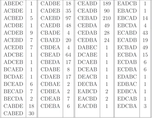
Rockmore in [39] re-discusses from a spectral theory point of view the data obtained by Thompson (see [43]) from the Catholic Charities Organitazion.
Catholic Charities sent out a questionairre to a sample of its members, ask-ing each participant to choose in order three of eleven possible charitable directions, that is an ordered 3–set from a 11–set.
To analyze such a study, many questions arise. Are people mainly choosing a favorite or two and then “randomly” choosing the rest? These would be first order considerations. Or are people’s choices driven by commonalities among the options? These are higher order effects.
We will explain in some part the spectral analysis approach to this data, which seeks to analyze the data as element of M(8,1,1,1), a representation
space of S11.
Let µ = (n − 1, 1). Then the Kostka numbers are Kλµ = h(λ) − 1, so,
according to Young’s rule (see theorem (1.3.4), Iλ,(n−1,1)∼= (h(λ)− 1)S(n−1,1).
The first row of the Young diagram of shape (n − 1, 1) can contain any string of nondecreasing entries, so that the only nonpermissible entry in the second row is 1. Thus, the various semistandard tableaux are determined by the entry in the second row which can be among 2, . . . , h(λ).
For example, for µ = (8, 1) and λ = (4, 2, 1, 1), we have Kλµ = 3, indeed
1 1 1 1 2 2 3 4 2 1 1 1 1 2 2 2 4 3 1 1 1 1 2 2 2 3 4 . So we have 3 copies of S(8,1) in M(4,2,1,1).
It is useful to give an illustration of the (n −1, 1) isotypic in terms of relevant characteristics of partially ranked data.
Partially ranked data of shape λ = (λ1, . . . , λk) can be viewed as frequencies
of respondents picking out their favorite λk items, then their favorite λk−1
items, and so on, all the way up to their least favorite λ items. Note that such a choice is determined by making only the first k − 1 sets of choices. Consider the following functions
∆(j)i (t) =½ 1 if t ranks i among the j
th favorites 0 otherwise Then ∆(j)i = 1 cij X δt
where cij is an appropriate normalization constant and the sum runs over all
It is not difficult to see that the functions {∆(j)1 , . . . , ∆ (j)
n } span a subspace
isomorphic to M(n−1,1). Following theorem (1.3.4), we have
M(n−1,1)∼= S(n)⊕ S(n−1,1).
S(n)is the subspace of constant functions and S(n−1,1) is its orthogonal
com-plement consisting of those functions whose values sum to 0.
Letting j vary from 1 to (n−1), we construct (n−1) subspaces which only in-tersect in the one–dimensional subspace of constant functions. These various subspaces of individual ranked popularity are naturally viewed as subspaces of the first order effects.
Data analysis. Spectral analysis may in general proceed into two steps: (1) first of all the coarse decomposition of the data vector f into its isotypic
components is considered
Having done (1), the lengths of the projection are considered. If a given projection has a large relative contribution then
(2) it is further investigated by considering some irreducible decomposition of particular isotypic.
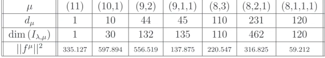
We are interested in the analysis of data of the shape (8, 1, 1, 1). Let f denote the original data vector. Theorem (1.3.4) gives us the decomposition of M(8,1,1,1) in
M(8,1,1,1) = S(11)⊕ 3S(10,1) ⊕ 3S(9,2)⊕ 3S(9,1,1)⊕ S(8,3)⊕ 2S(8,2,1)⊕ S(8,1,1,1) Analyzing data of the Catholic Charities, Rockmore obtained table (1.1) (see Rockmore, [39])
The isotypic decomposition indicates where the interesting projections are.
The large size of the (10, 1) projections suggests that this projection merits further analysis. We recall that this space measures the individual effects of the attraction (or repulsion) of individual charities.
To proceeds Rockmore follows the so–called Mallow’s method, which con-siders inner products of the projection with naturally interpretable functions
µ (11) (10,1) (9,2) (9,1,1) (8,3) (8,2,1) (8,1,1,1) dµ 1 10 44 45 110 231 120 dim (Iλ,µ) 1 30 132 135 110 462 120 ||fµ ||2 335.127 597.894 556.519 137.875 220.547 316.825 59.212 Table 1.1: Results
in the isotypics of interest (this method will be largely explained in Chapter 2. For references see [25]).
For the (10, 1)–isotypic one natural set of spanning functions are the ∆(j)i defined by
∆(j)i (t) =½ 1 if i is ranked in position j 0 otherwise
The following table gives the inner products of the (10, 1)–isotypic projection with {∆(j)i : i = 1, 2, 3, j = 1, . . . , 11} j 1 2 3 4 5 6 7 8 9 10 11 i 1 -37.4 -10.4 5.6 149.6 0.6 -12.4 -51.4 -6.4 -45.4 3.6 3.6 2 -28.4 9.6 28.6 59.6 10.6 -8.4 -43.4 -16.4 -42.4 43.4 -13.4 3 -34.4 22.6 37.6 8.6 7.6 -5.4 -31.4 -10.4 -31.4 28.6 7.6
Table 1.2: Results of Mallow’s method
A quick inspection of the entries of table (1.2) shows a very large (1, 4) entry, indicating that many respondents fell strongly about choosing charity 4 first. If we refer back to table (1.1), we notice that the counts for 3–tuples which first entry 4 are by and large the greatest.
Entries (3, 2), (2, 3), (3, 3), (2, 4), (2, 10), (3, 10) are of the next scale, indi-cating strong interest in charities 2, 3 and 10.
2
Spectral analysis and voting
Our work, exposed in Chapter 3, is an application of generalized spectral analysis to economic science and in particular to preference formation. It is modeled on some recent works of M. E. Orrison and B. L. Lawson (see [22], [23] and [24]) on noncommutative harmonic analysis of political voting. In this Chapter we want to illustrate this political application.
2.1
Noncommutative harmonic analysis of
vo-ting in committees
The kind of spectral analysis analyzed in section 1.5 of Chapter 1 is called generalized spectral analysis or also noncommutative harmonic analysis because it is a generalization of classical spectral analysis. Spectral analysis is the discrete Fourier analysis and it is basic for time series analysis and other types of analysis in the computational science, engineering and natural sciences. Diaconis (see [9] and [10]) extended the classical spectral analysis of time series to a non–time series subject, for the analysis of discrete data which has a noncommutative structure.
New efforts have been made in order to apply spectral analysis to a non– time series subject in the political sciences, above all in the analysis of voting.
Spectral analysis has been already used in political science to identify cy-cles in time series data. For example, spectral analysis was used to test if presidential popularity in the United State and the concentration of interna-tional power have periodic components.
Recently, M. E. Orrison and B. L. Lawson (see [22] and also [23], [24] with David T. Uminsky) introduced a generalization of spectral analysis as a new instrument for political scientist; they used the powerful machinery of spec-tral analysis to analyze political voting data. In particular, they analyzed votes of the nine judges of the United States Supreme Court (Warren Court 1958– 1962, Burger Court 1967–1981, Renquist Court 1994–1998) and de-tected influential coalitions.
With this theory political scientist can use spectral analysis as a method for identifying substantively important dynamics in politics, rather then just as a diagnostic tool.
The idea followed by Orrison and Lawson is to consider political voting data as elements of a mathematical framework; then the features of that framework can be used to work out natural interpretations of the data. The mathema-tical framework corresponding to voting data has many components, each of which encapsulates information on particular coalition effects; the decompo-sition of data with respect to these components provides the identification of influential coalitions.
2.2
Coalitions
Let X = {x1, . . . , xn} be a finite set and f : X −→ C a complex–valued
function on X. Let M be the vector space of all complex–valued functions on X and Sn the symmetric group of order n.
As already explained in section 1.2, M may always be decomposed into a direct sum
M = M0⊕ · · · ⊕ Mh (2.1)
for some positive integer h, where each Mi is an invariant subspace of M .
In particular, each function f ∈ M may be written uniquely as a sum f = f0+ · · · + fh (2.2)
with fi ∈ Mi and π(fi) ∈ Mi, for all π ∈ S.
There are many ways to decompose M as the direct sum of invariant sub-spaces; the idea behind spectral analysis is to choose the decomposition of M that provides invariant subspaces that encapsulate important properties of the data.
Suppose that X = {X1, . . . , Xn} is a set of n voters. Assume we have the
results of N non–unanimous votes and that each person casts a ballot on each vote. They define
X(n−k,k) = the set of k-elements subsets of the voters of X (2.3) with 1 ≤ k ≤ n
2 and denote with f(n−k,k) a function on X(n−k,k) defined as
f(n−k,k)(ω) = the number of times that ω is in the minority (2.4) for each ω ∈ X(n−k,k). Define
We observed that the permutations of Sn act on X, but also on the subsets
in X(n−k,k), for each k. Then, as outlined in equation (2.1), M(n−k,k) may be
decomposed as a direct sum
M(n−k,k) = M0⊕ M1⊕ · · · ⊕ Mk (2.5)
where each Mi is a subspace of M(n−k,k) invariant with respect to the action
of Sn. The space M0 is said to be corresponding to the mean response,
that is the average number of times an element of M(n−k,k)is in the minority.
M1 corresponds to the so–called first order effects, whereas Mi is related
to higher order effects, called coalition effects.
Spectral analysis focuses on the computation of the decomposition of each function f ∈ M(n−k,k) onto the components of (2.5), that is
f = f0+ · · · + fk. (2.6)
2.3
A five people committee
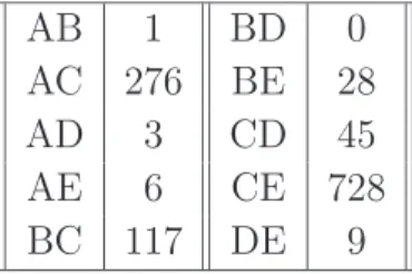
Let X = {A, B, C, D, E} be a committee of five people and suppose we have the results of 128 non–unanimous votes. Data is viewed as a function f defined on the subsets of X; in particular we have
f(4,1) = the number of times one person of X is in the minority. f(3,2) = the number of times two people of X are in the minority. Suppose that f(4,1) = 10 9 3 2 1 A B C D E and f(3,2) = 22 21 24 11 5 2 10 2 1 5 AB AC AD AE BC BD BE CD CE DE
This means that, in this example, A is in the minority against the other four people for 10 times, whereas AB are in the minority against the other three for 22 times, and so on.
Let M be the vector space of the complex–valued functions on X(4,1) and X(3,2); M may be naturally decomposed as
M = M(4,1)⊕ M(3,2),
where M(4,1) is the subspace of the functions on X(4,1) and M(3,2) on X(3,2). These two subspaces may be again decomposed into invariant subspaces
M(4,1)= M0(4,1)⊕ M1(4,1) (2.7) M(3,2)= M0(3,2)⊕ M1(3,2)⊕ M2(3,2). (2.8) We may project the functions f(4,1) and f(3,2) onto these invariant subspaces
and obtain
f(4,1) = f0(4,1)+ f1(4,1) (2.9) f(3,2) = f0(3,2)+ f1(3,2)+ f2(3,2). (2.10)
2.3.1
One person in the minority.
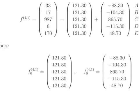
Going back to the example, according to decomposition (2.9), we get
f(4,1) = 10 9 3 2 1 = 5 5 5 5 5 + 5 4 −2 −3 −4 A B C D E where f0(4,1) = (5, 5, 5, 5, 5) f1(4,1) = (5, 4, −2, −3, −4)
The number of votes in which one person is in the minority is 25, so the average of the individual minority is 5 = 25/5; then f0(4,1)is the mean response
function. The function f1(4,1) shows the first order effect, which counts the
number of votes in which each person differs from the mean. In this case the interpretation of the first order effects doesn’t yield new information in relation to the initial data; the largest value is for A, that is most often in the minority, and the smallest value is for E, that is less often in the minority.
2.3.2
Two people in the minority.
We can appreciate the power of spectral analysis in the analysis of higher order effects. According to decomposition (2.10), we obtain
f(3,2) = 22 21 24 11 5 2 10 2 1 5 = 10.3 10.3 10.3 10.3 10.3 10.3 10.3 10.3 10.3 10.3 + 11.53 8.20 9.53 7.53 −4.80 −3.47 −5.47 −6.80 −8.80 −7.47 + 0.17 2.50 4.17 −6.83 −0.50 −4.83 5.17 −1.50 −0.50 2.17 AB AC AD AE BC BD BE CD CE DE where f0(3,2)= (10.3, 10.3, 10.3, 10.3, 10.3, 10.3, 10.3, 10.3, 10.3, 10.3) f1(3,2)= (11.53, 8.20, 9.53, 7.53, −4.80, −3.47, −5.47, −6.80, −8.80, −7.47) f2(3,2)= (0.17, 2.50, 4.17, −6.83, −0.50, −4.83, 5.17, −1.50, −0.50, 2.17) The function f0(3,2) is the mean response function; the number of votes in which two people are in the minority is 103, then the average of the minority of pairs is 10.3 = 103/10. The functions f1(3,2) and f2(3,2) capture the first order and second order effects. In order to interpret these effects, Orrison and Lawson [22] suggest to use Mallow’s method (see [25]).
2.3.3
Interpretation: Mallow’s method
To interpret the first order effects, for each subset of voters H, define a function fH ∈ M(3,2) which identifies the elements of f(3,2) “containing” H
with 1 and those “not containing” H with 0. In particular, fA= (1, 1, 1, 1, 0, 0, 0, 0, 0, 0)
fB = (1, 0, 0, 0, 1, 1, 1, 0, 0, 0)
fC = (0, 1, 0, 0, 1, 0, 0, 1, 1, 0)
fD = (0, 0, 1, 0, 1, 0, 0, 1, 0, 1)
fE = (0, 0, 0, 1, 0, 0, 1, 0, 1, 1)
The inner product between f1(3,2) and fH describes how much f (3,2)
1 lies in
the direction of H. Computing the inner products we get
fA fB fC fD fE
f1(3,2) 36.79 -2.21 -12.20 -8.21 -14.21
We observe that the first order effect lies most in the direction of A, being often in the minority with other voters, but lies least in the direction of E, being only occasionally in the minority of the pairs.
To interpret the second order effects, for each pair HK of X, define functions according to the criterion already explained, that is fHK ∈ M(3,2) identifies
the elements of f(3,2) which “contain” HK with 1 and the others with 0. So
fAB = (1, 0, 0, 0, 0, 0, 0, 0, 0, 0)
fAC = (0, 1, 0, 0, 0, 0, 0, 0, 0, 0)
fAD = (0, 0, 1, 0, 0, 0, 0, 0, 0, 0) etc.
fAE = (0, 0, 0, 1, 0, 0, 0, 0, 0, 0)
Computing the inner products between f2(3,2) and fHK we get the exact data
vector f2(3,2)
fAB fAC fAD fAE fBC fBD fBE fCD fCE fDE
f2(3,2) 0.17 2.50 4.17 -6.83 -0.50 -4.83 5.17 -1.50 -0.50 2.17 These results represents the pure second order effects, namely the pair’s weight in the minority, after removing the mean effects and the effects of the individual. The values of
f2(3,2) = 0.17 2.50 4.17 −6.83 −0.50 −4.83 5.17 −1.50 −0.50 2.17 AB AC AD AE BC BD BE CD CE DE represent the pair’s weight in the voting process.
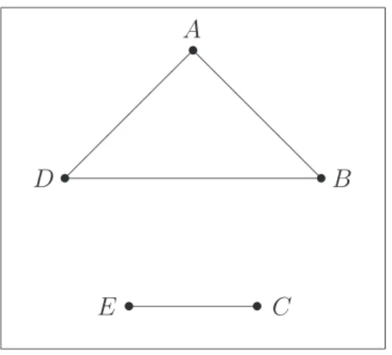
We observe that the second order effect lies most in the direction of BE and least in the direction of AE.
Through this analysis we may point out particular coalition effects that do not arise from a direct analysis of data; for example, the pair DE has a quite high second order effect, whereas D and E have low values in the first order effects of the minority related to the individual (f1(4,1)). This means that D and E are seldom in the minority alone, while they are often in the minority of the pairs.
2.4
Analysis of the Supreme Court
In [22] Orrison and Lawson used noncommutative harmonic analysis to de-tect and analyze coalitions in the United State Supreme Court.
This application seems very interesting because shows the power of the ma-chinery of generalized spectral analysis in detecting coalitions.
The United State Supreme Court has nine justices. So let X = {A1, . . . , A9}
be the set of the nine voters. The function f is defined on k-element subsets of X, with 1 ≤ k ≤ 4; this covers all cases since at most four justices can dissent on any given case. Unanimous cases are not considered.
Following the example of five people committee, if M is the vector space of all complex–valued functions on X, M decomposes into the direct sum of subspaces
M = M(8,1)⊕ M(7,2)⊕ M(6,3)⊕ M(5,4) These subspaces decompose into invariant subspaces
M(8,1) = M0⊕ M1
M(8,1) = M0⊕ M1⊕ M2
M(8,1) = M0⊕ M1⊕ M2⊕ M3
M(8,1) = M0⊕ M1⊕ M2⊕ M3⊕ M4
The difference with the example of section 2.3 is that here we have in addi-tion the projecaddi-tion on the subspaces M3 and M4; M3 contains information
about triples of justices and M4 contains information about groups of four
justices.
Orrison and Lawson analyzed voting of various Court: Warren Court from 1958 to 1962, Burger Court from 1967 to 1981, Renquist Court from 1994 to 1998. The analysis of these data is too long to be presented here; we refer to [22].