Università degli Studi di Sassari
Dipartimento di Agraria
Corso di Dottorato in Scienze Agrarie
Curriculum
Monitoraggio e controllo degli ecosistemi agrari e forestali
in ambiente mediterraneo
XXXI
C
ICLOInvestigation on lateral saturated soil hydraulic conductivity
evaluated at different spatial scales in a Mediterranean hillslope
Dott. Roberto Marrosu
Coordinatore del Corso Prof. Ignazio Floris Referente di Curriculum Prof. Alberto Satta Docente Guida Dott. Mario Pirastru Docenti Tutor Prof. Marcello Niedda
This dissertation is dedicated to Maria, who has encouraged me, loved and believed in me during the many years leading to this research dissertation.
Acknowledgments
This work would not have been possible without the dedication and support of numerous people.
First of all, I would like to thank my advisor Dott. Mario Pirastru and my tutor Dott. Mirko Castellini for the efforts that they have made to guide me during the doctoral studies.
My deep gratitude goes out to Prof. Marcello Niedda for giving me the opportunity to join the doctoral programme. “You are gone but your belief in me has made this journey possible”.
I especially would like to acknowledge Simone di Prima who spent many hours planning, digging and discussing site instrumentation, data analysis and data interpretation.
I also want to thank Ph.D. Ana Helena Dias Francesconi for her English teaching and precious advises.
A huge thanks goes out to my colleagues and friends Maria Grazia Farbo, Maria Teresa Tiloca, Angela Scanu, Elisa Campus and last, but not least, Giovanni Ragaglia for the support, endless patience and encouragements in this hard period. Each of them has left a mark in my life and for this I offer my very sincere gratitude to everyone. I wish them all the success, happiness, and joy in life.
Thesis index
Introduction 1
2. Objectives and thesis outline 5
3. References 7
Chapter 1
Subsurface flow and large-scale lateral saturated soil hydraulic conductivity in a
Mediterranean hillslope with contrasting land uses 12
1. Introduction 14
2. Material and Methods 17
2.1. Site description 17
2.2. Measurement of lateral subsurface flow 18
2.3. Estimation of the lateral saturated soil hydraulic conductivity 19
3. Results 20 3.1. Natural rainfall 20 3.2. Sprinkling experiment 26 4. Discussion 28 5. Conclusions 32 6. References 33 Chapter 2
Lateral saturated hydraulic conductivity of soil horizons evaluated in large-volume soil
monoliths 38
1. Introduction 40
2. Material and Methods 42
2.1. Location 42
2.2. Soil monolith preparation 43
2.3. Instrumentation 44
2.4. Drainage experiments 45
2.5. Ks,l calculation 46
4. Discussion 51
4.1. Benefits of the proposed field soil Ks,l assessment tool 51
4.2. Ks,l values of individual soil horizons 54
5. Conclusions 57
6. References 58
Chapter 3
In situ characterization of preferential flow by combining plot- and point-scale
infiltration experiments on a hillslope 63
1. Introduction 65
2. Material and Methods 69
2.1. Study site description 69
2.2. Soil sampling 69
2.3. In-situ block method 71
2.4. Modified cube method 74
2.5. BEST method 76
2.6. Dual-permeability approach 77
2.7. Data analyses 78
3. Results and discussion 79
3.1. In-situ and laboratory small-scale measurements 79
3.2. Comparing plot- and point-scale measurements 83
3.3. Lateral preferential flow 84
4. Conclusions 87
5. References 88
Chapter 4
Dependency of lateral saturated soil hydraulic conductivity from the investigation
spatial scale 97
1. Introduction 98
2. Methods 99
3. Results 100
List of figures
Fig. 1.1. View of the experimental hillslope, with location of the interceptor drains (ID) and spatial disposition of the piezometers at the FG and HM sites. The setup is not to scale. 17 Fig. 1.2. Boxplots of the water table depth in each well at the FG site for the years 2014 and 2015.
Only periods of natural rainfall are considered in the analysis. The boxes determine the 25th
and 75th percentiles, the whiskers are the 10th and 90th percentiles, the horizontal lines within
the boxes indicate the means. The dashed lines indicate the depth of the impeding layer as documented during well drilling. 21 Fig. 1.3. Boxplot of the hydraulic gradient, dZ/ds, values measured near the drain at the FG site for the
years 2014 and 2015. The statistical spread of mean hydraulic gradient used in Eq. (1) is also showed. The boxes determine the 25th and 75th percentiles, the whiskers are the 10th and 90th
percentiles, the horizontal lines within the boxes indicate the means. The dashed line indicates the local topographic gradient. 22 Fig. 1.4. a) Observed rainfall and b) observed drain outflow at the FG site and observed water table
depths in the wells C1, C2 and C3 during the natural rainfall events occurring from 2 to
5 February 2014. 23
Fig. 1.5. Water flow per unit width of drain, q, vs. water table depth, WTD3, values measured in the C3
and D3 wells of FG site for the natural rainfalls occurring in 2014–2015 years. The fitted exponential curve is also showed. 25 Fig. 1.6. a) Lateral saturated hydraulic conductivity, Ks,l, vs. water table depth values, WTD3, for the
natural rainfall occurring in 2014–2015 years. Average values of Ks,l computed for selected
water table depths are shown, together with the fitted exponential curve. b) Coefficients of variation (CV) of Ks,l for selected water table depths. 25
Fig. 1.7. Time series of the drain outflow observed during the sprinkling experiments in the FG and HM sites; circles indicate the end of water supply. 26 Fig. 1.8. a) Water flow per unit width of drain, q, vs. water table depth, WTD3, values measured in the
HM site during the transient and steady-state phases of the sprinkling experiments; b) lateral saturated hydraulic conductivity, Ks,l, vs. WTD3 estimated for the sprinkling experiments in
the HM site; c) q vs. WTD3 values measured in the FG site during the transient and
steady-state phases of the sprinkling experiment; d) Ks,l vs. WTD3 estimated for the sprinkling
experiment in the FG site. The continuous lines are the exponential functions fitted to the
q(WTD3) and Ks,l(WTD3) data estimated for the sprinkling experiments at the HM and FG
sites. The dashed line in the Figure 1.8d is the exponential function fitted to the Ks,l(WTD3)
data determined for the natural rainfall periods at the FG site, already shown in the
Figure 1.6a. 27
Fig. 1.9. Lateral saturated hydraulic conductivity, Ks,l, vs. water flow per unit width of drain, q, for
(a) the natural rainfall events of years 2014–2015 and the sprinkling experiment in the FG site, and (b) the sprinkling experiments in the HM site. 31 Fig. 1.10. Absolute percentage errors introduced in the estimate of the lateral saturated hydraulic
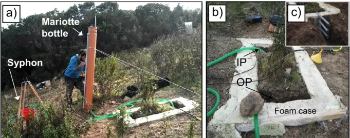
Fig. 2.1. Field equipment to determine lateral saturated soil hydraulic conductivities in the monoliths MA, MB and MC; (b) soil monolith encased with polyurethane foam, with signed inflow (IP) and outflow (OP) pits; (c) spillway pipes inserted in the OP foam of the monolith MD to set the water level and collect the drainage. 43 Fig. 2.2. Experimental design to estimate the lateral saturated hydraulic conductivity of soil horizons
from drainage of large-volume soil monoliths. The sketch represents the syphon system used in the MA, MB and MC monoliths to set the water levels and collect the drainage. 45 Fig. 2.3. (a,b) Time series of the inflow and outflow rates measured during the experiments in the soil
monoliths MA and MC; (c,d) computed differences between outflows and inflows. Note the difference in flow rate scale in the graphics. Numbers in squares indicate the following experiment stages: (1) soil saturation; (2) Mariotte bottle refilling; (3) water-level depth
transition. 49
Fig. 2.4. Computed specific Ks,l values in the A horizon and in the upper and lower layers of the
B horizon. The shaded area is the soil B horizon. 51 Fig. 3.1. Schematic diagram of a drainage experiment carried out on a soil block. Measured flows per
unit width of the block (qWTD) and thickness of the flow zones (TWTD) for different water table
depths (WTDs), distances along the sloping bed (s), and water table elevation from an
arbitrary datum (ΔZ). 72
Fig. 3.2. (a) Photo and (b) schematic view of the experimental setup of a drainage experiment carried
out on a soil block. 72
Fig. 3.3. Inflow (IF, open symbols) and outflow (OF, solid symbols) rates vs. time measured on the four soil blocks (SBs) at a water table depth (WTD) of 5 (blue rhombus), 15 (green circles)
and 25 cm (red triangles). 73
Fig. 3.4. Successive steps during the in situ extraction of the soil cube: (a) carving out the soil prism, (b) placing the wooden box to contain lateral foam expansion, (c) injecting polyurethane expandable foam between the box and the exposed soil and on the soil surface, and (d) positioning wood and a weight to prevent top foam expansion. 75 Fig. 3.5. (a) Cumulative empirical frequency distributions of the log-transformed saturated soil
hydraulic conductivity data, ln(Ks–BEST), obtained by the Beerkan method at the depths of 0, 5,
10, and 20 cm, and (b) ln(Ks–BEST) values plotted against the clay content (in %). The Pearson
correlation coefficient, r, is also reported. 80 Fig. 3.6. Impact of the fast-flow fraction, wf (-), on the saturated hydraulic conductivity for the
fast-flow region, Ks,f (mm h-1), estimated at different water table depths (WTDs) on the four soil
blocks (SBs). The reported wf values range from 0.05 to 0.1. 86
Fig. 4.1. Relationships between the investigated soil characteristic lengths and the median Ks,l values
List of tables
Table 2.1. Dimensions of the soil monoliths sampled in the drainage experiments. 44 Table 2.2. Arithmetic means of the outflow and inflow rates calculated over the last 30 min of the stages for each prescribed water-level depth. Inflows are in parentheses. The rates are in
mL·min−1·m−1. 48
Table 2.3. Lateral saturated soil hydraulic conductivities, Ks,l (mm·h−1), estimated from the drainage
experiments in the four soil monoliths for the water-level depths (WLD) of 5 cm, 15 cm and
25 cm from the soil surface. 50
Table 3.1. Clay (%), silt (%) and sand (%) content (U.S. Department of Agriculture classification), geometric mean particle diameter, dg (mm), dry soil bulk density, ρb (g cm−3), initial soil
water content, θi (cm3 cm−3), and saturated soil water content, θs (cm3 cm−3), for the four
sampled soil depths. The coefficients of variation (%) are listed in parentheses. 70 Table 3.2. Sample size, N, minimum, Min, maximum, Max, geometric mean, mG, standard deviation,
SD, and coefficient of variation, CV (%) of the saturated soil hydraulic conductivity,
Ks-BEST (mm h–1). All values were obtained using the Beerkan method at the depths of 0, 5,
10, and 20 cm. 80
Table 3.3. Sample size, N, minimum, Min, maximum, Max, geometric mean, mG, standard deviation,
SD, and coefficient of variation, CV (%) of the vertical, Ks,v–MCM (mm h-1) and horizontal,
Ks,h–MCM (mm h-1) saturated soil hydraulic conductivity values obtained by the constant-head
laboratory permeameter method on soil cubes (Klute and Dirksen, 1986). 81 Table 3.4. Geometrical dimensions and estimated saturated hydraulic conductivity, Ks–SB (mm h–1)
values for the four soil blocks. 84 Table 3.5. Estimated values of the saturated hydraulic conductivity for the fast-flow region,
Ks,f (mm h-1), for the lower (0.05) and upper (0.1) range values of the void ratio occupied by
the fast-flow region, wf (-), for the four soil blocks. 86
Table 4.1. Median values of lateral saturated soil hydraulic conductivity, Ks,l, determined for different
spatial scales of investigation for the A soil horizon , and for the upper (B1) and lower part
Introduction
The present research work focuses mainly on the estimation of the lateral saturated soil hydraulic conductivity, Ks,l, and on the quantification of lateral saturated subsurface flow
generated in a Mediterranean hillslope. The Ks,l is the key property governing groundwater
flow and the runoff generation process by saturation excess in steep shallow soils of watersheds. The most common initiation mechanism of lateral saturated subsurface flow (also known as subsurface stormflow) in a hillslope is the transient saturation of a vertical soil profile portion (Weiler et al., 2005). A perched water table originates from infiltrating rainwater that is hindered from deep downward percolation by a soil-bedrock interface or another layer of low permeability beneath the soil surface. Once the water table is formed, the water starts to flow laterally in direction to the toe of the slope. The spatial-temporal dynamics of the water table are mainly driven by the downslope water transfer velocities in the soil. The Ks,l, thus, is the soil hydraulic property that mostly determines the lateral
transmission rates of this saturated subsurface flow. As a consequence, the knowledge of reliable values of Ks,l is a prerequisite for properly interpreting the soil hydrological dynamics
related to subsurface flow. Consistent determinations of Ks,l are important in studies
evaluating the contribution of the subsurface stormflow to the volume of runoff discharge, or the transport of labile nutrients and pollutants from hillslope to the streams, surface reservoirs and aquifers (McGlynn and McDonnell, 2003; Tsuboyama et al., 1994; Zegre, 2003). Furthermore, subsurface flow is also reported as able to establish a positive pore water pressure in steep hillside (Montgomery and Dietrich, 2002; Schneider et al., 2014; Uchida et al., 2002, 2001, 1999; Wu and Sidle, 1995), which in turn can be a potential hydrological trigger for shallow landslides (Iverson, 2000; Montgomery et al., 1997; Schneider et al., 2014; Van Asch et al., 1999; Weiler et al., 2005). As these processes are intimately linked to the subsurface water flow velocities in the saturated soil, adequately Ks,l characterizing is of great
interest in hillslope hydrology.
Investigations on Ks,l and on the lateral saturated subsurface flow process in general, have
been undertaken mostly in watersheds of humid regions with steep slopes and shallow and conductive soils, where the subsurface flow often is acknowledged as the main mechanism of storm runoff production occurring on hillslopes. Conversely, in arid and semiarid regions this
process has received little attention, although recent studies have suggested that it plays a key role on hillslope hydrology even in these areas, including the Mediterranean ones (Maneta et al., 2008; Pirastru et al., 2014; van Schaik et al., 2014; Niedda et al., 2014). This was probably because in these environments lateral subsurface flow has traditionally been considered less important than surface hydrologic processes, since it is thought to occur only under certain extreme conditions (high rainfall depth and/or high antecedent soil moisture). Another reason is that measuring runoff in semiarid regions, compared to the humid temperate areas, faces more formidable challenges due to the particular climate features. In the former regions, in fact, the runoff producing events are rare and short-term; accordingly, time required for effectively characterizing runoff is relatively long-lasting, and occasions to make up for flawed monitoring strategy or equipment failures might be few and far between.
The Ks,l is the most important parameter in many numerical models that simulate water
flow processes both at hillslope and catchment scales (Dusek and Vogel, 2016; Hilberts et al., 2005). That models are used both for testing hydrological theories and for practical applications, such as assessing the effects of land-use or climate change scenarios on catchment hydrology. Successful numerical simulations require a good representation of the main processes affecting the dynamics of the hydrological system as well as reliable value estimates of model parameters. The Ks,l, as also pointed out by Flanagan and Nearing (1991),
is generally one of the most sensitive parameters in predicting runoff. For this reason, efforts should be directed towards a proper identification of this soil property value. Despite the fact that a number of methods are available for estimating the Ks,l in field and in laboratory, a
common practice among modellers is to calibrate the parameter value without attempts to experimentally estimate it. The main reason is that it is difficult to obtain representative values of Ks,l for large spatial scales (e.g., hillslope scale), which are generally those of
practical interest for distributed model applications, due to the high spatial variability that the saturated hydraulic conductivity exhibits (Warrick, 1998). Because of this variability, the experimental estimate of the soil Ks,l can vary over several orders of magnitude depending on
the sampled soil volume in the individual measurement (Chapuis et al., 2005). For instance, Vepraskas and Williams (1995) compared hydraulic conductivities measured on three different kinds of sample that differed in volume, namely undisturbed detached cores (3.5 x 10⁻⁴ m3), in situ columns (6.3 x 10⁻³ m3), and in situ drain fields (6.8 x 10⁻¹ m3) and
found that mean conductivity increased by about one order of magnitude passing from the small soil cores to the columns. However, Ks,l values obtained from the drain measurements
did not significantly differ from the column ones. Chappell and Lancaster (2007) determined Ks,l applying six field methods (i.e., slug test, constant- and falling-head borehole
permeameter, ring permeameter, and two types of trench tests). The large-scale Ks,l values
determined by the trench percolation tests were, on average, 37 times larger than the conductivity values obtained by slug tests made in wells placed near the trenches. The large-scale influence of soil structure, macropore flow and soil heterogeneity, were considered the main factors leading to these Ks,l discrepancies. In fact, when great soil volumes are
investigated a number of short and initially discontinuous preferential flow features (macropores, cracks, soil pipes, and root channels) are included in the soil sample. When the soil is then saturated, the soil matrix provides the connection between these discrete preferential features, organizing them into a more complex network (Anderson et al., 2008; Sidle et al., 2001). Such circumstance promotes fast lateral transfer of water and, consequently, high Ks,l values are determined through these measurements. Conversely, in
investigations performed on small volume soil samples such complex mechanism of macropore network activation may not become completely effective and, therefore, Ks,l values
lower than those detected in large sized soil samples are generally found. This suggests possible limitations in the usability of Ks,l determinations from small-size core-based
laboratory methods and near-point field infiltrometric techniques to characterize large hydrological units such as the hillslopes. For the same reasons, model users should be cautious when using Ks,l values measured in small soil samples without properly evaluating its
representativeness for large-scale modelling (Pachepsky et al., 2014). For example, Grayson et al. (1992) found that the base flow coming out of the Wagga Wagga catchment in New South Wales could be most accurately simulated by the THALES model by using an average Ks,l 10 times larger than the average measurement made with a disc permeameter. Wigmosta
et al. (1994) found that the ‘‘effective’’ lateral Ks,l determined by calibrating the DHSVM
model on the Middle Fork Flathead River basin in north-western Montana was 100 times the vertical soil conductivity estimated from pedo-transfer functions. Vertessy et al. (1993) demonstrated that the TOPOG_Yield was not able to accurately simulate streamflow without using a lateral Ks,l value roughly 10 times larger than the mean vertical Ks measured using
constant-head well permeameter. Once again, these discrepancies were attributed to the large-scale effects of macropore flow, which were not considered in the small-large-scale measurements. However, as Sherlock et al. (2000) suggested, calibrated Ks,l values greater than the
small-scale derived ones might also depend on compensations for the uncertainty of other calibrated hydrologic parameters in the model or could be linked to offsetting effects due to the simplified conceptual structure of the model. This indicates the need for identifying the most representative Ks,l value of the soil through appropriate experimental methods. The scale of
measurement should be comparable with the spatial discretization scale of the model, usually from tens to hundreds of meters of grid spatial resolution. Moreover, in order to elucidate scale-effects affecting the Ks,l determination in hillslope soils, measurement techniques and
strategies operating over a wide range of spatial scales have to be developed or improved. Experiments that seem to have a great potential for properly characterizing the hydrologic properties of large (square meters) to very large areas (tens of square meters) consist of excavating open trenches or installing drains to collect and measure the saturated subsurface flow moving above a confining layer in a hillslope. The reason is that the intercepted outflow integrates the hydrological response of the hillslope soil, which mostly depends on the flow through soil macropores (Beven and Germann, 2013; Chappell, 2010). On the other hand, these methodologies are too costly, time-consuming and difficult to conduct, thus remaining rare in literature. Whipkey (1965) measured hillslope-scale lateral flow and calculated Ks,l by
a trench experiment in an isolated hillslope. The Ks,l for the saturated soil was determined by
using Darcy’s law with reference to transient wetted cross-sectional area, the length of the saturated area, and the changes in hydraulic head over the entire saturated length. Similarly, Montgomery and Dietrich (1995) estimated the large-scale lateral Ks,l based on the discharge
from a gully cut which showed evidence of macropore flow. The authors observed that these determinations were comparable with the greatest conductivity obtained by falling-head tests in piezometers. Brooks et al. (2004) estimated the hillslope-scale Ks,l as a function of the
water table depth below the soil surface using drainage measurements performed on a 18-m wide isolated sloped land, reporting a hillslope-scale Ks,l values 3.2–13.7 times greater than
the available small-scale measurements.
Another possible way to determine representative Ks,l for large areas is to perform
impermeable material. For example, Day et al. (1998), who measured lateral water flow on a 3.38 m3 soil block, sealed the vertical faces of the block using bentonite, sand, and lumber.
Field procedures for evaluating the Ks,l in large soil samples are also reported by
Blanco-Canqui et al. (2002) and Mendoza and Steenhuis (2002). The latter developed and tested a device called “hillslope infiltrometer” by which the lateral drainage from each horizon of a layered soil was collected, and the specific lateral Ks,l values of the soil horizons
computed. Due to the increased exploited soil volume in the experimental approaches of Day et al.(1998), Blanco-Canqui et al. (2002) and Mendoza and Steenhuis (2002), an improved representation of the effects of soil heterogeneities compared with other near-point measurements would be expected. However, so far, only few cases of comparative analyses between Ks,l measurements performed in small soil samples (near-point spatial scale) and
those conducted in large volume soil blocks (plot scale) have been shown in literature (Blanco-Canqui et al., 2002). Furthermore, no comparative assessments of the Ks,l determined
at the plot scale and at the hillslope scale have been accomplished. Performing such comparisons could increase confidence in the measurements carried out by soil monolith approaches, like those of Day et al.(1998), Blanco-Canqui et al. (2002) and Mendoza and Steenhuis (2002), when these are used for large-scale applications.
2. Objectives and thesis outline
The main goal of the dissertation research was to investigate the changes of the lateral saturated soil hydraulic conductivity value estimations as a function of soil volume sampled with a given measurement technique. Indeed, different methods for the Ks,l determination
often yield substantially different Ks,l values because this soil property is extremely sensitive
to the sample size owing to heterogeneities of physical and hydrological soil characteristics. Comparing methodologically similar techniques, but dissimilar in involved measurement spatial scales, allows to better establish the usability of a given method for interpreting or modelling hydrological processes with reference to a specific scale of interest. By applying several methods involving diverse observational scales, the Ph.D. research is mainly aimed at gathering reliable Ks,l estimates that are representative for the hillslope scale. Moreover,
efforts are devoted to assessing the influence of the spatial scale of investigation on Ks,l
knowledge of representative Ks,l along the soil profile is an essential pre-requisite to
consistently simulate the spatio-temporal hydrological dynamics in soils.
The dissertation is structured in four chapters, three of them report research works published in international peer-reviewed journals.
Chapter 1 contains the manuscript titled “Subsurface flow and large-scale lateral saturated soil hydraulic conductivity in a Mediterranean hillslope with contrasting land uses”, which was published in Journal of Hydrology and Hydromechanics in 2017. The paper focuses on the lateral subsurface flow process characterization in two contiguous areas of a hillslope. An area was covered with natural maquis, the other one with grass. A continuous monitoring of the lateral saturated subsurface flow, collected at the footslope by drains, and of the water table levels, recorded in wells, was performed for two years. The investigation was mostly undertaken under natural rainfall regime, but also artificial rainfall experiments were carried out. Following the methodology introduced by Whipkey (1965) and Brooks et al. (2004) the hydrological data were used for computing Ks,l values along the
saturated soil profile. These values were considered representative for the large hillslope spatial scale, because the measured outflow by drains integrated the heterogeneous hydrological response of the hillslope soil. The specific objective of the research was to investigate the dependence of subsurface flow response from the soil use and to determine hillslope scale Ks,l values of the two sampled areas.
Chapter 2 reports the paper entitled “Lateral saturated hydraulic conductivity of soil horizons evaluated in large-volume soil monoliths” that was published in Water in 2017. The manuscript explores the suitability of drainage experiments performed on large volume soil monoliths to determine representative Ks,l values for macroporous steep soils. The monoliths
had an average soil volume of 0.12 m³, thus the sampled soil sizes were larger than the commonly sampled sizes by laboratory and field techniques, but smaller when compared to large scale, controlled drain experiments. The study aimed to refine a field technique to determine spatially representative Ks,l values of each soil horizon in the experimental
hillslope. Specific objectives were: i) to investigate the Ks,l variability along soil profile, and
ii) to evaluate spatial representativeness of Ks,l determined on monoliths at the studied site.
Chapter 3 reports the paper titled “In situ characterization of preferential flow by combining plot- and point-scale infiltration experiments on a hillslope”, published in
Journal of Hydrology in 2018. The paper proposes a new experimental approach to determine reliable parameters describing the hydraulic properties of the soil in both matrix and preferential flow (or fast-flow) regions. For this purpose, it was considered the dual permeability approach (i.e., the concomitance of fast- and matrix- flow in soils) and was computed Ks,l parameters for both flow regions. That was by coupling data from two kinds of
infiltration experiments performed at the near-point (Beerkan method and modified cube method) and at plot spatial scale (Ks,l measures by the soil monolith method). The aim was to
quantify the related contribution of the soil matrix and of the macropore network to the total lateral saturated subsurface flow.
Chapter 4 provides a comprehensive comparison of all the Ks,l determinations obtained at
different spatial scales by each methodology employed during the research work. The objective was to identify scale dependency relations of Ks,l as a function of the soil volume
sampled by the applied measurement techniques. Moreover, in this part insights are given about the technique for attaining, with the most sustainable experimental effort, representative Ks,l for the hillslope scale. Finally, concluding remarks of the dissertation research are
outlined.
3. References
Ameli, A.A., Amvrosiadi, N., Grabs, T., Laudon, H., Creed, I.F., McDonnell, J.J., Bishop, K., 2016. Hillslope permeability architecture controls on subsurface transit time
distribution and flow paths. Journal of Hydrology 543, 17–30.
https://doi.org/10.1016/j.jhydrol.2016.04.071
Anderson, A.E., Weiler, M., Alila, Y., Hudson, R.O., 2008. Dye staining and excavation of a lateral preferential flow network. Hydrology and Earth System Sciences Discussions, European Geosciences Union 5, 1043-1065.
Beven, K., Germann, P., 2013. Macropores and water flow in soils revisited. Water Resources Research 49, 3071–3092. https://doi.org/10.1002/wrcr.20156
Blanco-Canqui, H., Gantzer, C.J., Anderson, S.H., Alberts, E.E., Ghidey, F., 2002. Saturated Hydraulic Conductivity and Its Impact on Simulated Runoff for Claypan Soils. Soil
Science Society of America Journal 66, 1596–1062.
Brooks, E.S., Boll, J., McDaniel, P.A., 2004. A hillslope-scale experiment to measure lateral saturated hydraulic conductivity. Water Resour. Res. 40, W04208. https://doi.org/10.1029/2003WR002858
Chappell, N.A., 2010. Soil pipe distribution and hydrological functioning within the humid tropics: a synthesis. Hydrological processes 24, 1567–1581.
Chappell, N.A., Lancaster, J.W., 2007. Comparison of methodological uncertainties within
permeability measurements. Hydrological Processes 21, 2504–2514.
https://doi.org/10.1002/hyp.6416
Chapuis, R.P., Dallaire, V., Marcotte, D., Chouteau, M., Acevedo, N., Gagnon, F., 2005. Evaluating the hydraulic conductivity at three different scales within an unconfined sand aquifer at Lachenaie, Quebec. Canadian Geotechnical Journal 42, 1212–1220. Day, R.L., Calmon, M.A., Stiteler, J.M., Jabro, J.D., Cunningham, R.L., 1998. Water balance
and flow patterns in a fragipan using in situ soil block. Soil science 163, 517–528. Dusek, J., Vogel, T., 2016. Hillslope-storage and rainfall-amount thresholds as controls of
preferential stormflow. Journal of Hydrology 534, 590–605.
https://doi.org/10.1016/j.jhydrol.2016.01.047
Flanagan, D., Nearing, M., 1991. Sensitivity analysis of the WEPP hillslope profile model. Am. Soc. Agric. Eng. Paper.
Grayson, R.B., Moore, I.D., McMahon, T.A., 1992. Physically based hydrologic modeling: 1. A terrain-based model for investigative purposes. Water Resources Research 28, 2639–2658. https://doi.org/10.1029/92WR01258
Hilberts, A.G.J., Troch, P.A., Paniconi, C., 2005. Storage-dependent drainable porosity for
complex hillslopes. Water Resources Research 41:W06001.
https://doi.org/10.1029/2004WR003725
Iverson, R., M., 2000. Landslide triggering by rain infiltration. Water Resour. Res. 36, 1897– 1910. https://doi.org/10.1029/2000WR900090
Maneta, M., Schnabel, S., Jetten, V., 2008. Continuous spatially distributed simulation of surface and subsurface hydrological processes in a small semiarid catchment. Hydrological Processes 22, 2196–2214. https://doi.org/10.1002/hyp.6817
McGlynn, B.L., McDonnell, J.J., 2003. Role of discrete landscape units in controlling catchment dissolved organic carbon dynamics. Water Resources Research 39. https://doi.org/10.1029/2002WR001525
Mendoza, G., Steenhuis, T.S., 2002. Determination of hydraulic behavior of hillsides with a hillslope infiltrometer. Soil Science Society of America Journal 66, 1501–1504.
Montgomery, D.R., Dietrich, W.E., 2002. Runoff generation in a steep, soil-mantled
landscape. Water Resources Research 38(9), 1168.
https://doi.org/10.1029/2001WR000822
Montgomery, D.R., Dietrich, W.E., 1995. Hydrologic Processes in a Low-Gradient Source Area. Water Resources Research 31, 1–10. https://doi.org/10.1029/94WR02270
Montgomery, D.R., Dietrich, W.E., Torres, R., Anderson, S.P., Heffner, J.T., Loague, K., 1997. Hydrologic response of a steep, unchanneled valley to natural and applied rainfall. Water Resources Research 33, 91–109. https://doi.org/10.1029/96WR02985 Niedda, M., Pirastru, M., Castellini, M., Giadrossich, F., 2014. Simulating the hydrological
response of a closed catchment-lake system to recent climate and land-use changes in semi-arid Mediterranean environment. Journal of Hydrology 517, 732–745. https://doi.org/10.1016/j.jhydrol.2014.06.008
Pachepsky, Y.A., Guber, A.K., Yakirevich, A.M., McKee, L., Cady, R.E., Nicholson, T.J., 2014. Scaling and Pedotransfer in Numerical Simulations of Flow and Transport in Soils. Vadose Zone Journal 13. https://doi.org/10.2136/vzj2014.02.0020
Pirastru, M., Niedda, M., Castellini, M., 2014. Effects of maquis clearing on the properties of the soil and on the near-surface hydrological processes in a semi-arid Mediterranean
environment. Journal of Agricultural Engineering 45, 176–187.
https://doi.org/10.4081/jae.2014.428
Schneider, P., Pool, S., Strouhal, L., Seibert, J., 2014. True colors–experimental identification of hydrological processes at a hillslope prone to slide. Hydrology and Earth System Sciences 18, 875–892. https://doi.org/10.5194/hess-18-875-2014
Sherlock, M.D., Chappell, N.A., McDonnell, J.J., 2000. Effects of experimental uncertainty on the calculation of hillslope flow paths. Hydrological Processes 14, 2457–2471. Sidle, R.C., Noguchi, S., Tsuboyama, Y., Laursen, K., 2001. A conceptual model of
preferential flow systems in forested hillslopes: evidence of self-organization. Hydrological Processes 15, 1675–1692. https://doi.org/10.1002/hyp.233
Tsuboyama, Y., Sidle, R.C., Noguchi, S., Hosoda, I., 1994. Flow and solute transport through the soil matrix and macropores of a hillslope segment. Water Resources Research 30, 879–890. https://doi.org/10.1029/93WR03245
Uchida, T., Kosugi, K., Mizuyama, T., 2002. Effects of pipe flow and bedrock groundwater on runoff generation in a steep headwater catchment in Ashiu, central Japan. Water Resources Research 38. https://doi.org/10.1029/2001WR000261
Uchida, T., Kosugi, K., Mizuyama, T., 2001. Effects of pipeflow on hydrological process and its relation to landslide: a review of pipeflow studies in forested headwater catchments. Hydrological Processes 15, 2151–2174. https://doi.org/10.1002/hyp.281 Uchida, T., Kosugi, K., Mizuyama, T., 1999. Runoff characteristics of pipeflow and effects of
pipeflow on rainfall-runoff phenomena in a mountainous watershed. Journal of Hydrology 222, 18–36. https://doi.org/10.1016/S0022-1694(99)00090-6
Van Asch, T.W.J., Buma, J., Van Beek, L.P.., 1999. A view on some hydrological triggering systems in landslides. https://doi.org/10.1016/S0169-555X(99)00042-2
van Schaik, N.L.M.B., Bronstert, A., Jong, S.M. de, Jetten, V.G., Dam, J.C. van, Ritsema, C.J., Schnabel, S., 2014. Process-based modelling of a headwater catchment in a semi-arid area: the influence of macropore flow. Hydrological Processes 28, 5805–5816. https://doi.org/10.1002/hyp.10086
Vepraskas, M.J., Williams, J.P., 1995. Hydraulic Conductivity of Saprolite as a Function of Sample Dimensions and Measurement Technique. Soil Science Society of America Journal 59, 975–981. https://doi.org/10.2136/sssaj1995.03615995005900040003x Vertessy, R.A., Hatton, T.J., O’Shaughnessy, P.J., Jayasuriya, M.D.A., 1993. Predicting water
yield from a mountain ash forest catchment using a terrain analysis based catchment model. Journal of Hydrology 150, 665–700. https://doi.org/10.1016/0022-1694(93)90131-r
Warrick, A.W., 1998. Spatial variability. In: D. Hillel, Editor. Environmental Soil Physics, San Diego: Academic Press, 655–675
Weiler, M., McDonnell, J.J., Meerveld, I.T., Uchida, T., 2005. Subsurface Stormflow, in:
Encyclopedia of Hydrological Sciences. American Cancer Society.
https://doi.org/10.1002/0470848944.hsa119
Whipkey, R.Z., 1965. Subsurface stormflow from forested slopes. Hydrological Sciences Journal 10, 74–85.
Wigmosta, M.S., Vail, L.W., Lettenmaier, D.P., 1994. A distributed hydrology-vegetation model for complex terrain. Water Resources Research 30, 1665–1679. https://doi.org/10.1029/94WR00436
Wu, W., Sidle, R.C., 1995. A Distributed Slope Stability Model for Steep Forested Basins. Water Resources Research 31, 2097–2110. https://doi.org/10.1029/95WR01136 Zegre, N.P., 2003. The hillslope hydrology of a mountain pasture: The influence of
subsurface flow on nitrate and ammonium transport. Virginia Polytechnic Institute and State University.
CHAPTER 1
Subsurface flow and large-scale lateral saturated soil
hydraulic conductivity in a Mediterranean hillslope with
contrasting land uses
Mario Pirastru1, Vincenzo Bagarello2, Massimo Iovino2, Roberto Marrosu1, Mirko Castellini3,
Filippo Giadrossich1, Marcello Niedda1
1 Dipartimento di Agraria, Università degli Studi di Sassari, Viale Italia 39, 07100, Sassari, Italy
2 Dipartimento di Scienze Agrarie e Forestali, Università degli Studi di Palermo, Viale delle Scienze, 90128,
Palermo, Italy
3 Consiglio per la ricerca in agricoltura e l’analisi dell’economia agraria – Unita di ricerca per i sistemi
colturali degli ambienti caldo-aridi (CREA–SCA), Via Celso Ulpiani 5, 70125, Bari, Italy
Published in: J. Hydrol. Hydromech., 2017, 65(3), 297-306.
Abstract. The lateral saturated hydraulic conductivity, Ks,l, is the soil property that mostly
governs subsurface flow in hillslopes. Determinations of Ks,l at the hillslope scale are
expected to yield valuable information for interpreting and modeling hydrological processes since soil heterogeneities are functionally averaged in this case. However, these data are rare since the experiments are quite difficult and costly. In this investigation, that was carried out in Sardinia (Italy), large-scale determinations of Ks,l were done in two adjacent hillslopes
covered by a Mediterranean maquis and grass, respectively, with the following objectives: i) to evaluate the effect of land use change on Ks,l, and ii) to compare estimates of Ks,l
obtained under natural and artificial rainfall conditions. Higher Ks,l values were obtained
under the maquis than in the grassed soil since the soil macropore network was better connected in the maquis soil. The lateral conductivity increased sharply close to the soil surface. The sharp increase of Ks,l started at a larger depth for the maquis soil than the
grassed one. The Ks,l values estimated during artificial rainfall experiments agreed with those
obtained during the natural rainfall periods. For the grassed site, it was possible to detect a stabilization of Ks,l in the upper soil layer, suggesting that flow transport capacity of the soil
pore system did not increase indefinitely. This study highlighted the importance of the experimental determination of Ks,l at the hillslope scale for subsurface modeling, and also as
a benchmark for developing appropriate sampling methodologies based on near-point estimation of Ks,l.
Keywords: subsurface runoff, drain, pore connectivity, sprinkling experiments, land use
1. Introduction
Lateral saturated subsurface flow is the dominating runoff generation mechanism in most hillslopes or catchments of the humid temperate climates (Weiler et al., 2005) but it also occurs in many semiarid regions (Newman et al., 1998; Niedda and Pirastru, 2013; Van Schaik et al., 2008).
The most suitable approach for studying the mechanisms that govern the subsurface response of vegetated hillslopes consists of excavating open trenches or installing drains to intercept and measure directly the saturated subsurface flow moving above an impeding layer. The reason is that the measured outflow integrates the heterogeneous hydrological response of the soil in the hillslope, which can be governed by flow through the spatially and temporally variable soil macropores (Beven and Germann, 2013; Chappel, 2010). The primary role of the macropores in determining timing, peak and volume of the generated subsurface flow has been demonstrated in different large-scale investigations, that were primarily carried out in humid or temperate climates (Anderson et al., 2009; Dusek et al., 2012; Jost et al., 2012; Uchida et al., 2004). For example, Anderson et al. (2009) found that the hydraulic connectivity of the preferential flow network at the hillslope scale was an important factor governing subsurface flow, and they were able to determine relationships between lateral flow, hillslope length and various storm indicators. Uchida et al. (2004) found that hillslope discharge during storms was mainly due to macropore flow, which was strongly related to the cross-sectional area of the upslope saturated layer.
In semi-arid regions, subsurface processes have traditionally been considered less important than surface flow for discharge production. However, models which explicitly simulate lateral saturated subsurface flow in hillslopes (Maneta et al., 2008; Niedda and Pirastru, 2015; Van Schaik et al., 2014) suggest that subsurface flow plays a key role on catchment-scale hydrology even in semi-arid regions. In any case, little information is still available about the dominant mechanism of subsurface flow generation in many semiarid environments, including the Mediterranean ones. For these regions, there is the need to sample subsurface flow in natural hillslopes and to establish sources of spatial and temporal variability.
lateral water transport in hillslopes and it is a key parameter in many numerical models that simulate hydrological processes both at the hillslope (Dusek and Vogel, 2016; Hillbert et al., 2005) and catchment (Maneta et al., 2008; Matonse and Kroll, 2013; Niedda et al., 2014) scales. For example, Ks,l has to be known to estimate soil erosion with the modified
Morgan-Morgan-Finney model by Morgan and Duzant (2008). The Ks,l data used for modeling
purposes should be determined in agreement with the considered flow direction. In fact, anisotropy can determine saturated conductivity differing, even greatly (four orders of magnitude or more), with the considered direction (e.g., Bathke and Cassel, 1991; Beckwith et al., 2003; Bouma and Dekker, 1981; Dabney and Selim, 1987). This circumstance is relevant for interpreting soil hydrological processes (Montgomery and Dietrich, 1995).
A variety of approaches can be found in the literature to determine Ks,l. For example,
approximate criteria, based on soil textural characteristics alone (e.g., Ks,l = 2100 mm h-1 for a
sandy loam soil according to Morgan and Duzant, 2008), can be used. However, these values should be used with caution, being unverified. Various experimental techniques have been applied for small-scale estimates of Ks,l. These techniques include constant- and falling-head
borehole permeameter techniques specifically developed for radial flow (Reynolds, 2010; 2011) and measurements on soil monoliths (Baxter et al., 2003; Blanco-Canqui et al., 2002; Chappell and Lancaster, 2007). Other methodologies have been developed with the specific objective to sample large to very large (dozens of m2) areas, but only a few investigations of
such a type can be found in the literature (Brooks et al., 2004; Chappell and Lancaster, 2007; Montgomery and Dietrich, 1995). The Ks,l determinations obtained with large-scale
experiments can be expected to allow an improved representation of heterogeneity effects on the hillslope hydrological response as compared with near-point measurements. The scarcity of large-scale investigations is due to the fact that the experiments are expensive and difficult to conduct. Brooks et al. (2004) determined the hillslope-scale Ks,l as a function of the water
table depth below the soil surface using drainage measurements performed on a 18 m wide isolated sloped land. These authors found that Ks,l increased abruptly near the surface, due to
the activation of flow in the near-surface macropores of biological origin. The reported hillslope-scale estimation of Ks,l was 3.2–13.7 times greater than the available small-scale
measurements. Montgomery and Dietrich (1995) estimated the large scale Ks,l based on the
were comparable with the greatest conductivity obtained by falling-head tests in piezometers. Chappell and Lancaster (2007) applied six field methods (i.e., slug test, constant- and falling-head borehole permeameter, ring permeameter, as well as two types of trench tests) to determine Ks,l. The large-scale Ks,l values determined by the trench percolation tests were, on
average, 37 times larger than the mean conductivity obtained by slug tests made in piezometers adjacent to the trenches.
Greater values of Ks,l, even by several orders of magnitude as compared with those
determined at the point-scale, can be found when hydrological models are calibrated using the observed hydrologic response of the catchment (Blain and Milly, 1991; Chappell et al., 1998; Grayson et al., 1992). These discrepancies were generally attributed to the large-scale effects of macropore flow. However, Sherlock et al. (2000) also suggested that the differences between the measured and calibrated hydraulic conductivities could be linked to offsetting effects of the conceptual simplifications of the applied hydrological model, as well as to error effects of the other parameters involved.
In summary, our experimental knowledge of lateral subsurface flow processes in semi-arid environments is still incomplete notwithstanding that there are signs that these processes can be relevant even in these environments. Large-scale experiments are rare in general although they represent an efficient way to obtain directional soil hydraulic properties functionally averaging local heterogeneities.
This study focuses on the lateral subsurface flow processes in a hillslope with a different vegetation cover in the semiarid Mediterranean climate. A continuous monitoring of the lateral saturated subsurface flow and of the water table levels was carried out for two years in two contiguous areas, one covered with natural maquis and the other covered with grass established after the maquis clearing. The specific objective was to determine the subsurface flow response and the lateral saturated soil hydraulic conductivity of the two sampled hillslopes under both natural and artificial rainfall.
2. Material and Methods
2.1. Site description
The study was performed in the Baratz Lake catchment (Giadrossich et al. 2015; Niedda et al., 2014; Pirastru and Niedda, 2013), in North-West Sardinia, Italy. The climate is semiarid Mediterranean, with a mild winter, a warm summer and a high water deficit between April and September. The mean annual temperature is 15.8 °C and the mean relative humidity is 78.7%. The minimum and maximum mean daily temperatures are 3 °C and 29 °C, respectively. The average annual precipitation is about 600 mm, and this falls almost all from autumn to spring. The potential evapotranspiration is around 1000 mm year-1.
The experimental area was on the steep side of a hill (Figure 1.1). It has a mean elevation of 63 m a.s.l. and it is about 60 m long. The sloped surface is roughly planar, faces north and has a mean gradient of 30%. In the upper part, the incoming overland and subsurface flows are diverted by the ditches alongside a road. At the foot, the hillslope is drained by the incised stream of the main river of the catchment area.
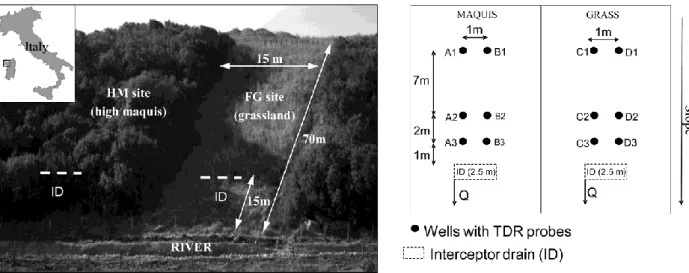
Fig. 1.1. View of the experimental hillslope, with location of the interceptor drains (ID) and spatial disposition of the piezometers at the FG and HM sites. The setup is not to scale.
Two adjacent sites in the hillslope were selected for the research. One site is covered with a well-developed Mediterranean maquis (hereafter named HM site). It consists of a very dense growth of evergreen trees and shrubs with a height of 2–4 m composed by
Myrtus Communis L., Arbutus unedo L., Erica arborea L., Phillirea latifolia L. and Pistacia lentiscus L. A litter at least 10 cm thick overlies the mineral soil at this site.
The other site is an unmanaged area covered with spontaneous grass (hereafter named FG site). This area developed about 15 years ago, after maquis clearing and mouldboard ploughing to create a 15 m wide firebreak.
The soil in the hillslope is Lithic Haploxerepts. It is about 0.4–0.5 m deep and overlies a grayish, altered substratum of Permian sandstone, which is very dense. This impeding layer limits deep water percolation. The soil texture is sandy-loam according to the USDA standards.
Field observations at the sites indicate that macropores due to grass or tree roots and animal burrows are mainly present near the surface. Detailed information about the hydraulic characteristics of the soils in the HM and FG sites are reported in Castellini et al. (2016) and Pirastru et al. (2014).
2.2. Measurement of lateral subsurface flow
Continuous hydro-meteorological data were collected at the experimental site from January 2014 to December 2015. The gross rainfall was measured every 5 minutes by a tipping bucket rain gauge (0.2 mm of resolution) in an automatic weather station 500 m away from the studied hillslope. The lateral saturated subsurface flow above the impeding layer was collected by two 2.5 m long French drains that were installed 15 m from the slope foot, as shown in Figure 1.1. At the FG site, the drain was installed centrally to the grassed area, and at the HM site it was about 10 m far from the lateral maquis border. Outflow from each drain was routed in a plastic box which outlet is a 60° V-notch weir. The water head over the V-notch was measured by a stand-alone pressure transducer every 5 minutes, and related with the flow rate by the weir formula. The outgoing flow from the box dropped into an automated tipping bucket (about 2·10-3 l/tip), thus providing a more accurate measure of the flow rate
when this was smaller than 0.4 l min-1.
Twelve piezometers were hand-drilled until the impeding layer was reached (Figure 1.1). On each hillslope, six wells were grouped in two adjacent transects positioned upslope and perpendicular to the drain. Within a transect, three wells were spaced at a distance of 1, 3 and 10 m from the drain. As a convention, the transects were denoted by the letters from A to D
and the wells in each transect were progressively numbered from the top to the bottom (Figure 1.1). Each well had a diameter of 80 mm and it was screened by 0.3 m above the top of the impeding layer. The depth of the soil, as documented when drilling the wells, ranged from 0.35 to 0.45 m at the FG site, and from 0.38 to 0.44 m at the HM site. The wells were equipped with automated TDR probes (Campbell Scientific Inc. CS216 Water Content Reflectometers, two-rod model, 0.3 m rod-length and 32 mm spacing), standing vertically in the wells, whose output was recorded every 5 minutes. As the probe rods were short compared to the soil thickness, they were periodically moved up or down in the wells to maintain them always partially submerged. The relationship between the TDR output and the percentage of rod submergence was calibrated in the laboratory. This relationship, with the reference depth of the probe, was used to determine water table depths. These data were validated through manual measurements of water table depths collected in the field during site visits. The mean absolute error between the values of water level estimated by the calibrated TDR output and those measured manually in the field was less than 1 cm, and this error was considered negligible for the purposes of the investigation.
On April 2014, artificial rainfall was applied once at the FG site and twice at the HM site. In each site, a network of irrigation sprinklers was arranged in an area about 12 m long and 8 m large, located immediately upslope of the interceptor drain and including all the monitoring wells. At the HM site, irrigation water was applied below the trees to exclude interception by tree canopy.
In this site, a steady rainfall of 40 mm h-1 was applied for about 2.75 h on April 1. This
irrigation was mainly made with the aim of increasing the soil moisture of the irrigated plot to a level comparable to that observed at the FG site. Two days after, a steady rainfall of 60 mm h-1 was applied for 2.7 hours at both the FG and HM sites.
2.3. Estimation of the lateral saturated soil hydraulic conductivity
The observed groundwater levels and the drained subsurface flow were used to estimate the lateral saturated soil hydraulic conductivity, Ks,l [L T-1], according to Childs (1971) and
Brooks et al. (2004). In particular, Childs (1971) presented a solution to groundwater flow to a transverse ditch or tile line over a sloping impermeable bed. Brooks et al. (2004) applied the Childs (1971) solution to compute Ks,l at an isolated sloping plot 35 m long and 18 m wide.
Assuming that the groundwater flow lines are parallel to the bed, following the Dupuit-Forchheimer approximation, flow of water per unit width of the drain, q [L2T-1], can
be modelled by means of the Darcy’s law:
− = ds dZ T K q s,l (1)
where T [L] is the thickness of the saturated layer, measured perpendicular to the impermeable bed, Z [L] is the water table elevation from an arbitrary datum, and s [L] is the distance along the hillslope. In this investigation, q, T, and dZ/ds were measured during field monitoring or determined using simple geometry. In this way, Eq. (1) can be solved directly to obtain a relation between Ks,l and the water table depth below the soil surface.
3. Results
3.1. Natural rainfall
Cumulative rainfall was 550 mm in 2014 and 528 mm in 2015. For the analysis, rainfall events were considered distinct if they were separated by at least 6 hours without rain, and events with less than 3 mm in six hours were disregarded. About eighty events, ranging in depth from 3.2 to 91 mm, occurred between January 2014 and December 2015. At the FG site, subsurface flow was observed during 80% of these events, mainly occurring during the autumn and spring periods. The maximum and the mean outflow volumes were about 3.6 m3
and 1.3 m3, respectively, and the maximum outflow rate was 11.7 l min-1. At the HM site,
drainage was less frequent than at the FG site and the collected water volumes were scarce. In particular, the drain intercepted subsurface flow for 40% of the rain events. The maximum and the mean collected water volumes were 0.3 and 0.05 m3, respectively, and the maximum
outflow rate was 2 l min-1. Therefore, only few information about K
s,l were obtained for the
maquis soil. Considering the weak hydrological response of the HM site under natural rainfall, the hydraulic characterization of this site was only based on the artificial rainfall experiments.
At the FG site, a water table developed in autumn and spring only as a consequence of the greatest rainfall events. In winter, with high rainfall and low evapotranspiration, a water table steadily formed in the hillslope and, due to the high soil wetness, even small rainfall
events caused piezometer responses. Figure 1.2 shows a boxplot of the observed water table depths at the FG site. On the contrary, the piezometer responses were almost absent at the HM site throughout the monitored period. For consistency of the analysis, only periods when all instruments were simultaneously functioning were considered. Lack of data was due to malfunctioning of some device or to water level fluctuations greater than those measurable by the TDR probes. Data from all instruments were simultaneously available for the 80% of the time during the period of occurrence of drain outflow.
Fig. 1.2. Boxplots of the water table depth in each well at the FG site for the years 2014 and 2015. Only periods of natural rainfall are considered in the analysis. The boxes determine the 25th and 75th
percentiles, the whiskers are the 10th and 90th percentiles, the horizontal lines within the boxes indicate
the means. The dashed lines indicate the depth of the impeding layer as documented during well drilling.
The water table in the C3 well was the deepest on both years whereas the water levels in the D2 and D3 wells were the closest to the soil surface. The observed similarity between the two years of observation suggests that there was a temporal stability in the groundwater spatial dynamics in the hillslope. The piezometer responses were consistent between wells
located at the same elevation in the hillslope. On both years, the lowest Spearman correlation coefficients, ρ, were detected with reference to the water levels in the C2 and D2 wells (ρ = 0.81 in 2014 and ρ = 0.92 in 2015) whereas the highest ρ values were obtained for the C3 and D3 wells (ρ = 0.96 and 0.95, respectively).
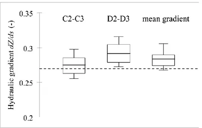
Figure 1.3 shows a boxplot of the hydraulic gradients, dZ/ds, estimated from the water levels in the wells located 1 and 3 m far away the drain along the two established transects. The gradients used for Ks.l calculation (Eq.1) were computed as the arithmetic mean of the
hydraulic gradients along the two transects near the drain. Only the wells near the drain were considered in order to have a more accurate estimate of the gradients that effectively drove the drain response. Figure 1.3 shows the statistical spread of the dZ/ds values. Generally, the hydraulic gradients were close to the topographic gradient, and deviations from this latter did not exceed 5% in most cases.
Fig. 1.3. Boxplot of the hydraulic gradient, dZ/ds, values measured near the drain at the FG site for the years 2014 and 2015. The statistical spread of mean hydraulic gradient used in Eq. (1) is also showed. The boxes determine the 25th and 75th percentiles, the whiskers are the 10th and 90th percentiles, the
horizontal lines within the boxes indicate the means. The dashed line indicates the local topographic gradient.
The relationship between water table depth and outflow was investigated in detail by checking the hydrological response of the hillslope during a sequence of distinct rainfall events. Figure 1.4b shows the response of the drain and the water levels in the three wells of transect C for the period from February 2 to February 5, 2014. Data from a single transect were considered for this analysis due to the detected consistence between well data for the
two transects and also because similar results to those reported in Figure 1.4b were obtained by either considering transect D or averaging the two transects (data not shown). Lateral subsurface flow was almost absent on February 2, when 5 mm of rainfall caused a large fluctuation of the water table close to the C3 well but levels in the C1 and C2 wells varied by only a few centimeters. Seven and 8 mm of rainfall fell on February 3 and 4, respectively. The water level in the C3 well fluctuated and peaked, with a behavior similar to that observed for the previous event. For the C1 and C2 wells, water levels closer to the soil surface were observed. Both amount and peak of the outflow showed a variation between events larger than the variation in fallen rain. Therefore, a rise in water level in the C3 well alone was not enough to collect significant subsurface runoff volumes. Instead, the water table rise close to the soil surface in the drained area was a necessary condition for generation of considerable subsurface flow. A possible physical interpretation of this finding is that higher water levels increased hydraulic connectivity of the soil pore system.
Fig. 1.4. a) Observed rainfall and b) observed drain outflow at the FG site and observed water table depths in the wells C1, C2 and C3 during the natural rainfall events occurring from 2 to 5 February 2014.
The time correspondence between water table level fluctuations and drain outflow response was also detected when peaks in both drain outflow and water table rise were well identifiable (Figure 1.4b). In general, the increase of water table started simultaneously in all wells and the time when levels peaked also coincided among wells. The drain outflow dynamics closely followed the water table dynamics. In fact, outflow started to increase when water table began to respond, and the outflow and water table levels peaked at the same time.
To establish the best estimate of the saturated layer thickness, T, to be used in Eq. (1), an estimate of the water table depth, WTD, at a given elevation along the hillslope was obtained by averaging the two water level values and the correlation between q and WTD was checked. The lowest correlation between q and WTD (ρ = 0.86) was found for the 2014 data and the wells farther away from the drain (C1 and D1). The highest correlation was obtained by considering the closest wells to the drain (WTD3, i.e., the average of the C3 and D3 well
levels), since ρ was close to 0.93 on both years. Therefore, WTD3 was used for the calculation
of T in Eq. (1).
Taking into account the similarity of the relationships between q and WTD3 for the two
monitored years, a single q(WTD3) relationship was developed by considering the q(WTD3)
data of both years. This relationship was clearly non-linear (Figure 1.5). Above the depth of about 0.17 m (small thickness of the saturated layer), q varied by 2×10⁻⁴ l s-1m-1 per
centimeter of WTD fluctuation. Below this depth (thicker saturated layer), q variation per unit change in water table depth was 25 times greater. This result suggested that Ks,l greatly
increased in the upper soil layer.
The highest estimated Ks,l values were close to 3000 mm h-1 for a WTD of about 0.1 m
(Figure 1.6a). Similar results (i.e., Ks,l = 3600 mm h-1) were obtained by Montgomery and
Dietrich (1995) in a soil presenting the evidence of macropore flow. The rate of change of Ks,l
with WTD increased by more than one order of magnitude in the passage from small (i.e., WTD > 0.17 m) to large saturated soil layers. Figure 1.6b shows that the Ks,l data were more
prone to uncertainty (higher coefficients of variation, CV) for small water table levels (high WTD values). This result was a consequence of the relatively poor correlation between q and WTD for the high WTD values (Figure 1.5). A low correlation between the trench outflow and the water table depth for low subsurface flow regimes was also observed in other experimental hillslopes (Anderson et al., 2009; Uchida et al., 2004). The observed trend of Ks,l
as a function of WTD3 was satisfactorily modelled by an exponential function (Figure 1.6a).
This model is in agreement with the assumption of many hydrological models, such as TOPMODEL (Ambroise et al., 1996), that the soil transmissivity exponentially increases with the thickness of the saturated soil layer.
Fig. 1.5. Water flow per unit width of drain, q, vs. water table depth, WTD3, values measured in the
C3 and D3 wells of FG site for the natural rainfalls occurring in 2014–2015 years. The fitted exponential curve is also showed.
Fig. 1.6. a) Lateral saturated hydraulic conductivity, Ks,l, vs. water table depth values, WTD3, for the
natural rainfall occurring in 2014–2015 years. Average values of Ks,l computed for selected water
table depths are shown, together with the fitted exponential curve. b) Coefficients of variation (CV) of
3.2.Sprinkling experiment
At the HM site, the first sprinkling experiment (rainfall intensity = 40 mm h-1) was
carried out on an initially dry soil. The drain took about one hour to respond to the rainfall input. The outflow increased throughout the duration of the experiment, until q = 0.085 l s-1 m-1 was reached at the end of the experiment (Figure 1.7). The total collected
water volume was 1.6 m3 and the runoff coefficient was 0.5. Surface runoff did not occur
during the experiment.
Fig. 1.7. Time series of the drain outflow observed during the sprinkling experiments in the FG and HM sites; circles indicate the end of water supply.
The second, more intense (rainfall intensity = 60 mm h-1) sprinkling experiment was
carried out while the drain was slowly leaking. The drain responded about 30 minutes after irrigation started. Subsurface flow increased for an hour up to a steady rate of about 0.12 l s-1 m-1, which did not vary during the subsequent hour. The collected subsurface water
volume was 2.25 m3, which represented about 51% of the total supplied water volume.
Surface runoff generated during this experiment, and its water volume was about 8% of the supplied water volume.
The two sprinkling experiments at the HM site yielded similar q(WTD3) relationships
(Figure 1.8a). A complete saturation of the soil layer was never achieved, being 0.08 m the minimum reached water table depth. For a water table depth greater than about 0.25 m the drain response was almost absent while above this depth the outflow was highly responsive to