Implementation of a sort-last volume rendering using 3D textures

UNIVERSIT `

A DI PISA

Facolt`a di Scienze Matematiche, Fisiche e Naturali Corso di Laurea Specialistica in Informatica

Implementation of a sort-last

volume rendering using 3D textures

Master Thesis

Author:

Matteo Salardi

Advisors:

Prof. Thilo Kielmann

Dr. Paolo Cignoni

Acknowledgements

The main part of the implementation described in this work was accomplished at the Vrije Unversiteit of Amsterdam. I am extremely grateful to Prof. Thilo Kielmann, for the great opportunity he gave to me. I am grateful to Tom van der Schaaf, for his endless patience and skillful support. I thank the Vrije Universiteit, since for several months i used its facilities. I wish to thank Dr. Paolo Cignoni and the Department of Computer Science of Pisa, which allowed me to prepare my master thesis abroad.

The University of Pisa supported this thesis with a scholarship. The rest was provided by my parents and my gung-ho grandmothers. I am deeply grateful to all of them.

1 Introduction 1

2 Volume rendering 5

2.1 Introduction and indirect techniques . . . 5

2.1.1 Overview . . . 5

2.1.2 Volume slicing . . . 7

2.1.3 Indirect volume rendering . . . 8

2.2 Direct volume rendering . . . 10

2.2.1 Ray casting . . . 10

2.2.2 Splatting and cell projection . . . 12

2.2.3 Shear-warp . . . 14

2.2.4 Texture-based rendering . . . 14

2.3 State of the art . . . 16

2.3.1 Hybrid methods . . . 16

2.3.2 Unstructured grids . . . 18

2.3.3 Large and dynamic data set . . . 20

2.4 Software . . . 23

2.4.1 OpenGL and 3D textures . . . 23

Contents ii

2.4.2 Aura and 3D textures . . . 25

3 Parallel volume rendering 29 3.1 Parallel rendering . . . 29

3.1.1 Clusters of commodity components . . . 29

3.1.2 Molnar’s taxonomy . . . 30

3.1.3 Sort-first . . . 31

3.1.4 Sort-middle . . . 33

3.1.5 Sort-last . . . 35

3.2 State of the art . . . 36

3.2.1 Complex hierarchical structures . . . 36

3.2.2 Out-of-core and multi-threaded approach . . . 38

3.2.3 Hybrid sort-first/sort-last approach . . . 40

3.3 Software for parallel rendering . . . 42

3.3.1 Chromium . . . 42

3.3.2 Parallel rendering with Chromium . . . 44

3.3.3 Parallel rendering with Aura . . . 46

4 Implementation of a sort-last rendering in Aura 49 4.1 Code design . . . 49

4.1.1 Aura internals . . . 49

4.1.2 OpenGL buffers . . . 52

4.1.3 Read and write operations on buffers . . . 54

4.1.4 Project structure . . . 56

4.1.5 Aura SortLastProcessor . . . 58

4.1.7 DisplayServer . . . 60

4.2 Slicing and compositing . . . 60

4.2.1 Slicing algorithm . . . 60

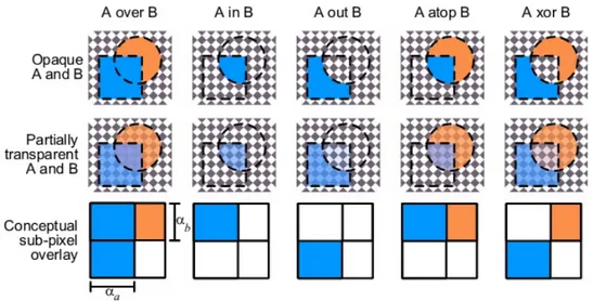
4.2.2 Alpha compositing . . . 61

4.2.3 OpenGL alpha blending . . . 65

4.2.4 3D compositing via stencil buffer . . . 66

4.2.5 3D compositing without depth information . . . 68

4.3 Parallel compositing . . . 69

4.3.1 Parallelism at the compositing phase . . . 69

4.3.2 Direct send . . . 70 4.3.3 Parallel pipeline . . . 70 4.3.4 Binary swap . . . 71 5 Validation 74 5.1 Analysis . . . 74 5.1.1 Overall analysis . . . 74

5.1.2 Parallel compositing analysis . . . 76

5.2 Tests . . . 77

5.2.1 Cluster overview . . . 77

5.2.2 Tests . . . 78

Chapter 1

Introduction

The present work describes an implementation of a parallel volume rendering, accomplished by extending an existing graphics library, Aura, and employ-ing the OpenGL API. The volume renderemploy-ing is a field belongemploy-ing to the more general area of computer visualization, that is the efficient rendering onto a display of a certain data set, in order to better understand and investigate properties and structures of the data set. The branch of visualization tech-niques concerning volumetric data set is the volume rendering. This work is implemented using the 3D texture method, that is a volume rendering technique which takes advantage of the new hardware facilities of modern graphics boards. This approach is coherent with state of the art works, since a truly interactivity can be achieved only exploiting the underlying hardware. The reason to adopt a parallel solution is the need for processing data set that are larger than the ones supported by a standard graphics board. A cluster of PCs was used to test the volume rendering, according with recent research trends. Actually clusters are preferred to customized high-end workstations,

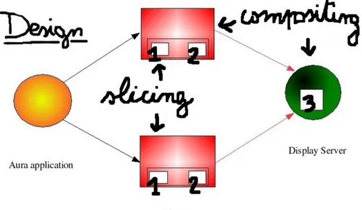
basically because clusters of commodity components are cheaper and inher-ently easier to upgrade. Sort-last is the parallel model adopted, that is the original 3D texture is distributed among the nodes of the cluster, and it is splitted in a slicing phase. Each node is in charge of rendering its part of the volume, then the framebuffer of each node is read and sent to a node which performs the final compositing phase. Special cares are necessary if the final compositing also requires alpha blending. A binary swap algorithm among the nodes is implemented too. The binary swap allows to reduce the compositing bottleneck that is generated when all the entire framebuffers are sent to the same final node.

Chapter 2 exposes the main techniques in volume rendering. In sec-tion 2.1 a short overview is provided, where the main applicasec-tion fields are pointed out. It is introduced the first and simplest technique, the volume slicing. Section 2.1.3 is about the indirect volume rendering, where the data set is first fitted with geometric primitives and then is rendered. The aim is to approximate with the geometry a certain iso-surface of interest, then the rendering is achieved feeding the graphics board with the geometric primi-tives. The basic algorithm for performing an indirect volume rendering is the marching cubes. Section 2.2 presents the other main class of algorithms for volume rendering, that is the direct volume rendering. The main difference with the indirect techniques is that the data set rendering is achieved without any intermediate geometry. The main techniques are ray casting, splatting, cell projection, shear-warp and finally the hardware based texture mapping. Section 2.3 describes the state of the art. Recent research trends tend to ex-ploit the new GPUs features and to achieve volume rendering for large data

3

set. Thus an algorithm is presented which intensively use the programmable shaders to perform an hybrid method made up of texture mapping and ray casting. Furthermore, the main issues related to irregular data set, out-of-core algorithm and dynamic data set are presented. Section 2.4 shortly describes the OpenGL API and its functions to create a 3D texture. Finally the Aura graphics library is introduced.

Chapter 3 deals with parallel volume rendering, since several techniques have been proposed to exploit hardware made of multiple computational nodes. Section 3.1 presents an overall analysis of parallel rendering, first com-paring the hardware support given by high-end graphics workstations with clusters of commodity components. The Molnar’s taxonomy, a landmark for classification of parallel rendering algorithms, is introduced, followed by a deeper description of its three main classes: first , middle and sort-last. Section 3.2 points out state of the art techniques and research trends in parallel rendering. Hierarchical data structures are a preferred way to man-age large data set, especially when it has to be distributed among several nodes. The multi-threaded approach is also widely employed. An hybrid algorithm which fall into both sort-first and sort-last classes is described. Its performance overcomes the traditional sort-first or sort-last algorithms in many cases. Section 3.3 presents software related to the parallel render-ing. The Chromium library is widely accepted as the outstanding software for parallel rendering. Aura, used for our work, also supports the parallel rendering.

Chapter 4 concerns our implementation of a sort-last volume rendering using the Aura library. Section 4.1 is about the design choices taken to

add the new components to Aura. First an overview of the Aura internal structure is given. The OpenGL buffers system and the read and write operations on buffers are described. The project design is motivated and the new components are introduced. Section 4.2 is about the slicing strategy adopted in our work and the compositing phase. The alpha compositing theory is introduced, according to the Porter and Duff results. OpenGL implementation of the alpha compositing is given. Alpha compositing in the 3D domain is generally achieved using the stencil buffer. However our implementation can avoid the use of the stencil buffer. Section 4.3 deals with the parallel compositing issue. The need for parallelism at the compositing phase is pointed out. Three algorithms are proposed: direct send, parallel pipeline and binary swap. The latter is the one adopted in our work.

Chapter 5 gives validation results. Chapter 6 presents the final consider-ations and gives suggestions for future works.

Chapter 2

Volume rendering

2.1

Introduction and indirect techniques

2.1.1

Overview

Scientific visualization of volumetric data is required in many different fields of interest. Medical applications are an obvious example. Several tools are nowadays available to obtain image data from different angles around the human body and to show cross-sections of body tissues and organs. The pur-pose is to support the physician diagnosing internal disorders and diseases. The computed tomography (CT) scanner consists of a large machinery with a hole in the center, where a table can slide into and out. Inside the machine an x-ray tube on a moving gantry fires an x-ray beam through the patient body, while rotating around it. Each tissue absorbs the x-ray radiation at a different rate. On the opposite side of the gantry a detector records this 1D projection, after a 360-degrees rotation around the body a computer can

compose all the projections to reconstruct a 2D cross-sectional view of the body, or slice. The table advances and the same procedure is repeated for the new section, until the interesting area is completely scanned and a set of 2D slices is ready. Besides CT, magnetic resonance (MR) and ultrasound imaging are widespread methods to produce a digital representation of the human internals.

There are also other scientific areas which require to handle huge amounts of image data. The goal is still to improve the knowledge of the data set achieving a high-quality rendering and allowing a flexible and efficient ma-nipulation. Numeric simulations in physics as computational fluid dynamics are a good example. In sophisticated molecular modeling, oceanographic experiments or meteorological simulations the parameters needed to be in-vestigated are associated with shades of gray or, more commonly, with RGBA colors. Generally speaking, all the areas concerning the study of a scalar field can find an important support representing the 3D domain as a volumetric data set:

f : D1 ⊂ <3 → D2 ⊂ <

Using a different and more convenient terminology, the data set is rep-resented as a 3D array of scalar values, or voxel grid. Each of the elements of the array is called voxel. The function which describes how the voxels are spaced determines the grid type. The simplest case is of course the constant function, where each voxel is regularly spaced (i ∗ d, j ∗ d, k ∗ d or i ∗ dx, j ∗ dy, k ∗ dz) and thus the grid is called regular. Otherwise the grid is curvilinear (x[i], y[j], z[k] or also x[i, j, k], y[i, j, k], z[i, j, k]). The grid is referred to as unstructured if no function can be given to describe the voxels

2.1. Introduction and indirect techniques 7

position.

Since real world data sets are usually generated and stored using the scale of greys, it is necessary to map each voxel to a RGBA color, in order to highlight the wished elements of the data set. This task is accomplished using one or more transfer functions, which associate a RGBA value to a grey one. For instance, the skin of a human hand has a certain constant value on the scale of greys. The transfer function can be used to highlight the skin, associating to its value a bright RGBA color. If we prefer to investigate the hand internals the skin can be mapped to a transparent color (i.e, the alpha value is set to zero). In the next paragraphs a short taxonomy of the main techniques adopted in the volume rendering field is provided.

2.1.2

Volume slicing

The main task of a visualization application is to reduce the volumetric data set to a 2D image, since the output is usually displayed on a 2D surface. The simplest way to achieve such result is to extract a planar 2D slice from the volume and to directly show it onto the screen, I(x, y). Of course with this technique the data loss is enormous, all the advantages to exploit the spatial organization of the data is lost. A method to partially overcomes this problem is to show several slices simultaneously, or in a temporal sequence

I(x, y, t) = f (α1x, α2y, t)

In this case time replaces the missing spatial coordinate. Otherwise it’s possible to display several slices at the same time, using also orthogonal

cut-ting to allow the user to mentally reconstruct the three dimensional relations of the volume. Orthogonal slices can also be embedded together to improve the general comprehension of the volume.

2.1.3

Indirect volume rendering

A second approach is represented by the indirect volume rendering (IVR), also referred to as surface rendering. Data are converted in a set of polygons, and then rendered using the standard graphics hardware, typically able of efficient rendering for geometric primitives. Here the main task is to detect the surfaces of interest, and then to fit the volume with the appropriate prim-itives. The surface is usually identified with a constant value, or iso-value, so only the voxels of our volumetric data set with this value are displayed.

f (x, y, z) = k, k constant

Cuberilles was one of the first widely used methods for this purpose [12], the basic idea is to use a binary segmentation to determine which voxels belong to the surface and which do not. All the voxels of the object are then joined together to approximate the final surface. If the number of voxels is not large enough the final image can look like it’s made up of squared bricks. To improve the image quality the original data set can be re-sampled increasing the number of voxels, but this implies at the same time to increase the computation time.

The well-known marching cubes algorithm is an important evolution of this technique, proposed by [21]. In this case the volume is organized in

2.1. Introduction and indirect techniques 9

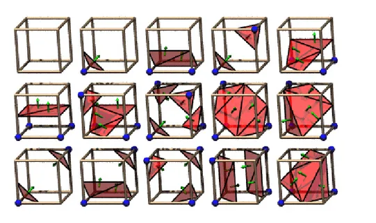
Figure 2.1: Marching cubes basic combinations. Source: http://groups.csail.mit.edu/graphics/classes/6.838/F01/lectures/Smooth Surfaces/0the s047.html

cubes made up of 8 voxels. The goal is to detect which ones of the 8 voxels of each cube belongs to the iso-surface, and then to create the appropriate triangular patches which divide the cube between regions within the iso-surface and regions outside. At each step a cube is classified with an index for the values of its corners, potentially the combinations are 256 but a strong simplification exploiting symmetries gets only 15 combinations. The index is used to look up a precalculated table and to obtain the correct patches, then vertexes are interpolated and the normal is calculated. Finally, the surface representation is obtained by connecting the patches from all cubes.

Although marching cubes is a standard and wide used method for IVR, many improvements were proposed to overcome unexpected behaviors due to ambiguous cases. One way is to add 6 new combinations to the original 15 to remove ambiguities. Another way is the marching tetrahedra algorithm,

where tetrahedra are used instead of cubes to detect surfaces. A finer detail is provided and the arising of ambiguous cases is avoided.

2.2

Direct volume rendering

2.2.1

Ray casting

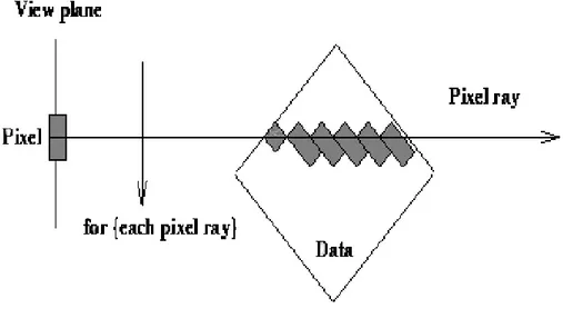
Another approach is the direct volume rendering, also simply known as vol-ume rendering. The data set is directly projected onto the 2D viewing plane without fitting visible geometric primitives to the samples. The data set is represented as a kind of 3D cloud. The basic styles are ray casting, splat-ting, cell projection, shear-warp projection and texture-based mapping, but it’s common to combine these ground techniques to obtain hybrid methods. Ray casting [19] is a special case of the more complex ray tracing method. A ray is fired from every pixel in the image plane into the data volume, and for this reason ray casting is classified as an image-order approach. Along the intersection of the ray with the volume shading algorithms are performed to obtain the final color of the pixel, using a back-to-front order for the final composition. The contribution of each data sample to the pixel depends on a set of optical properties, like color, opacity, light sources, emission and reflection model. A first advantage compared to the IVR is that the vol-ume shading is free of any classification of the voxels, while only the voxels detected as belonging the surface are rendered in the IVR, resulting in fre-quent false positives (spurious surfaces) or false negatives (unwished holes in surfaces).

2.2. Direct volume rendering 11

Figure 2.2: A ray is fired through the volume. Source: http://smohith.tripod.com/proj/vhp/thesis/node92.html

opacity value. But ray casting is an extremely computation intensive process, that’s why many improvements have been proposed to increase the perfor-mance. The main remark is there are usually many transparent regions (i.e., opacity is zero) inside the volume, they do not give any contribute to the final image but they are processed as significant ones. Transparent regions can be skipped modifying the ray casting algorithm with the hierarchical spacial enumeration [20]. An additional pyramidal data structure is required. All the voxels are grouped together into cells of different sizes, the minimum with the same size of a single voxel and the maximum with the size of the entire volume. Each cell also contains links to parents and children cells and a value set to one if there are children of the cell with an opacity greater then zero, zero otherwise. So when a ray is cast the pyramidal structure is traversed starting from the biggest cell and at each step the cell value is tested. The

voxels on the base are reached and shaded only if all the cell parents get a one as result, if a zero is encountered it means there is a transparent region. Another optimization can be accomplished avoiding inner regions with an high opacity coefficient when the ray has already accumulated an opacity value close to one processing the data. A threshold is set and if it is reached the ray can be terminated, further voxels would not be visible.

Ray casting is also employed to implement a different technique which does not belong to the DVR algorithms, the maximum intensity selection (MIP). The basic concept is to select the maximum value along with each ray, in such a way only a little subset of voxels contribution to the final image. This can be useful to depict a specific structure from the volume ignoring the rest, as blood vessels in a data set produced by a MR scanner. MIP exists in many variants as local MIP, where the first value above a given threshold is selected. Furthermore, MIP can be joined with a DVR technique to obtain a hybrid method.

2.2.2

Splatting and cell projection

Splatting, first proposed by [38], is an object-order approach, either back-to-front or back-to-front-to-back; pixel values are accumulated by projecting footprints of each data sample onto the drawing plane. This method processes only objects existing in the volume, avoiding transparent regions. It’s particularly efficient for sparse data sets. To skip opaque inner regions is more difficult, because a voxel which doesn’t contribute to a certain footprint can contribute to another one.

2.2. Direct volume rendering 13

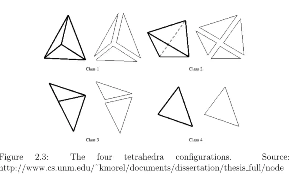
Figure 2.3: The four tetrahedra configurations. Source: http://www.cs.unm.edu/˜kmorel/documents/dissertation/thesis full/node 28.html

as the projected tetrahedra of [31]. The volume is first decomposed in tetra-hedrical cells which are then classified according with the viewpoint vector. Tetrahedrons were chosen as the cell-shape because they are the simplest possible polyhedron (4 vertices, 6 edges and 4 faces) and because they are simple (non self-intersecting) and convex. Any kind of simple polyhedron can be decomposed in a set of tetrahedrons. Furthermore, a tetrahedron projected onto a plane can be broken into triangles, only four configurations are possible. Thus once a tetrahedron is classified it can be decomposed with triangles, values are linearly interpolated and then the triangles are rendered. All the above methods are high quality methods with similar performance, with a better behavior of splatting for sparse volumes and with an easier parallel implementation for ray casting. The next methods have a lower quality but they are faster.

2.2.3

Shear-warp

A third method is shear-warp [16]. It is a hybrid technique which traverses both image and object space at the same time. Unlike ray casting, the pro-jection of the data set onto the surface is splitted in two different steps, a shearing along the axis of the volume and a final 2D warp operation. The sheared volume is projected on a base plane, normal to an axis of the volume coordinate; the goal of the shearing phase is to simplify the projection op-erations, that usually represent the computational bottleneck in many algo-rithms, like ray casting. Finally the warp step corrects the image distortion, due to the angle between the base plane and the viewing plane. To accelerate the shear-warp rendering usually run-length encoding is used for sequences of voxels with similar properties, for example for transparent regions. All the pixels covered by the projection of a run are treated equally, increasing the performance.

2.2.4

Texture-based rendering

Texture-based methods are a last approach, which takes advantage of the texture mapping hardware. Although all the above basic methods can reach important results and many efforts have been done to further improve their performances, a truly real time DVR cannot be achieved only via a software solution. If only 2D textures are available, we consider three axis aligned sets of slices of the volume, each applied as 2D texture; the set that is most perpendicular to the viewing direction is selected and alpha-blended in a back-to-front order. Otherwise, if 3D textures are supported, only one set

2.2. Direct volume rendering 15

Figure 2.4: 3D texture. Source: [14]

of slices is necessary. They are constructed aligned in the object space or, more likely, in the image space (i.e., perpendicular to the viewing direction) and placed within the volume. Slices are then rendered using a trilinear interpolation for the slices coordinates, using color and opacity values from the volume loaded into the texture memory. To achieve the final rendering the slices are blended together, again in a back-to-front order.

Since its first introduction the hardware based approach could overcome long term performance issues related to volume rendering. In order to fully understand its success it is worth noting that nowadays the power of GPUs is increasing faster then the power of CPUs, thus there is a huge availability of cheap and powerful graphics boards. However, data set size is also increasing fast, and the texture memory available on a graphics board represents a strong constraint to the hardware based approach. Moreover, this method produces several fragments which may not contribute to the final image, as seen for other techniques such as ray casting.

2.3

State of the art

2.3.1

Hybrid methods

Recent works usually propose hybrid methods, where the good performances of hardware based texture mapping are combined with the advantages of other methods. [14] intensively exploit the new features available on the new generation of graphics boards, that is programmable shader units, high band-width to access the texture memory and high parallelism inside the rendering pipeline, in particular with the presence of several fragment units. The ba-sic idea is to generate slices textured with color and opacity from the data set as in the standard hardware based texture mapping, and then to adopt ray casting to skip inner regions and empty voxels or to detect iso-values. In order to implement such method the hardware support has to allow the redirection of the rendering process to a 2D texture (used to store the in-termediate results, the texture is aligned with the viewport and it has the same resolution), to allow the generation of texture coordinates (to access slices and temporary textures while a ray is traversing the volume) and to calculate arithmetic operations (but also more complex ones as dot product) in the shader programs, and finally to allow a fragment to change its depth value.

The method requires four passes:

1. Entry point determination. The front faces of the volume are rendered and stored in a temporary 2D RGB texture (TMP). The color values represent the 3D texture coordinates, thus the first intersection of the rays of sight with the volume.

2.3. State of the art 17

2. Ray direction determination. The same procedure is executed for the back faces of the volume, the rays direction and length are computed and stored in a 2D RGBA texture (DIR), where the RGB components are used for the normalized direction and the A component for length. 3. Ray traversal and early ray termination. Rays are casted through the volume and the accumulated value is determined at each pass. The tex-tures generated at the previous steps TMP and DIR are used as lookup tables, while another 2D texture (RES) is employed to store interme-diate results. The early ray termination is easily performed testing the current ray length with the length stored in the A component of DIR. If the ray exits the volume the corresponding A component in RES is set to 1. The iso-surface detection can be performed traversing the volume from back-to-front at this pass. When the current ray value is equal or greater to a certain iso-value it is stored on a temporary variable. 4. Stopping criterion. The A component in RES related to the current ray

is compared with a threshold value, if it is greater the respective depth value is set to a maximum value, otherwise to 0. The idea is to avoid useless computations using the z-buffer test. The same idea can be fruitful employed to perform an empty space skipping. An additional 3D RGB texture is needed to store octree hierarchy information. It corresponds to a particular octree level with nodes of constant size. The minimum and maximum value of the child nodes (i.e., the bounds of the region covered by the octree node) is stored in the R and G components. This extra 3D texture is used to address a 2D texture, where for each

pair R/G it is shown if there are non-zero color component inside, that is for each region it indicates if it is empty or not. The empty space skipping test can be performed together with the threshold test, if an empty region is detected the fragment depth value is set to the maximum value (but whenever a non empty region is found is reset to 0).

2.3.2

Unstructured grids

Besides algorithms exploiting new GPUs features as seen above, many al-gorithms have been developed to apply DVR techniques tailored for regular grids to unstructured ones. The irregular data set is usually represented by a tetrahedral mesh, that is a set of tetrahedra where for each pair of tetrahedra is possible to determine if they are disjoint, incident or adjacent. However meshes made of other types of cells are also possible, such as hybrid meshes made of tetrahedra and irregular hexahedra. A first issue is to perform a visibility ordering on the cells, that is a total order such as if cell A obstructs the cell B for a given viewpoint, then B precedes A in the ordering. The visibility ordering is essential to achieve a correct final result and it is useful to efficiently exploit the graphics hardware.

A first object oriented approach is the Meshed Polyhedra Visibility Or-dering (MPVO), where an adjacency graph is computed from the mesh. Ba-sically, each node of the graph correspond to a cell, and the edge between two nodes represents a shared face. The shared face defines a plane which divides the space into two half spaces, each containing one of the two nodes. The edge is oriented towards the node lying on the same half space of the

2.3. State of the art 19

viewpoint, thus the entire graph can be oriented and the visibility ordering achieved.

An opposite, image oriented approach is the A-buffer, where the ordering is performed after the rasterization. Each primitive is rasterized without any concern about the ordering, then the generated fragments are stored in a per-pixel linked list containing the depth values. The depth values are then used to sort the list. The main disadvantage of the A-buffer method is it requires extra memory to store the linked lists.

An hybrid approach is represented by the k-buffer, which combines the previous methods. A first approximate ordering is performed by the CPU on the cells, then the primitives are rasterized and a further ordering is performed by the GPU using the k-buffer. The main difference between the A-buffer and the k-buffer is that while the A-buffer memory requirements are unbounded since linked lists are stored on the A-buffer, the k-buffer requires a constant amount of memory, that is k entries are stored for each pixel. Each entry contains the distance of a fragment from the viewpoint, it is used to sort the fragments.

After the visibility ordering is accomplished the standard DVR methods can be adopted as for regular grids. It is worth noting DVR of an unstruc-tured grid is much easier if all the cells are convex, otherwise problems can arise sorting the cells and applying the conventional algorithms (e.g., a ray traversing a non-convex mesh with ray casting enters and exits a cell more then once). Convexication of a mesh can be performed, nowadays it is still a hard task though.

2.3.3

Large and dynamic data set

The need for processing large data set represents another outstanding area of interest, since data set size increases faster then hardware support. A first method is to simplify the data set in order to obtain a data set that is easier to handle. This is usually achieved with a pre-processing step, however it produces a static approximation, thus it can introduce artifacts. If a texture based method is being used, the pre-processing can split the original texture into several bricks, detect and discard the empty regions and finally rearrange the 3D texture. A more refined method consists in using hierarchical data structure to provide a multi-resolution or level-of-detail (LOD) representation of the data. [36] adopts this approach combined with the 3D texture based technique. The texture is divided into several bricks, then for each brick a set of coarser approximations is computed, thus a multi-resolution hierarchy structure is generated. Only the more interesting regions of the data set are rendered at the higher resolution, the less significative areas are loaded and rendered at a coarser resolution, reducing the impact of the trilinear interpolation and thus improving the interactivity.

Although all the above techniques allow to treat large data set, modern applications and scientific experiments may need to handle even larger data set, overwhelming the standard PC resources. This happens when the data set have been generated by a supercomputer but the visualization process has to be accomplished on a PC or a mid-range workstation. A solution to this issue is addressed by the out-of-core approach, that is to use the disks in order to overcome the main memory limits. The out-of-core approach was not first employed by computer visualization, since it was already adopted for

2.3. State of the art 21

computational problems in science and engineering, which do not fit inside the main memory, and for the database field, which is inherently out-of-core. The main overheads introduced are due to the communication bottle-neck between the disk and the memory and to the inefficient random access to the disk, because each seek operation implies the movement of mechanical parts. Thus the out-of-core approach is required to overcome such overheads, usually providing an ad-hoc data structure to organize and efficiently handle the data set on disk. For instance, [6] restructure the original data set using an octree during a pre-processing step. The octree is recursively generated inserting at each phase the cells into the octree node. When a node needs to be splitted because it contains an exceeding amount of cells it creates its children and distributes the cells among them. If a cell could intersect more than one node it is replicated. After the pre-processing, the octree is used to load only the required portion of the data set on demand. [8] propose two out-of-core algorithms for DVR of large unstructured grids. The first is a memory-insensitive rendering that requires only a small amount of main memory. The basic idea is to pre-process the files containing the vertexes and cells lists in order to avoid random access to the disk. Then each cell is transformed and traversed by a ray, the intersection is computed and stored when the ray enters and exits the cell. The sampled values are then sorted, so all the values concerning the same pixel are grouped together, in a sequential order, ready to be employed for the compositing phase. The second algorithm is an extension of the in-core ZSWEEP, which basically sweeps the data with a plane parallel to the view plane increasing the z coordinate. All the cells incident to vertices are projected onto the plane, the contribute they give

to each pixel is stored in a sorted list, the data structure adopted is similar to the A-buffer. When the sweeping plane reaches a target z coordinate the compositing is performed. The out-of-core ZSWEEP divides the data set in chunks, so only a subset is loaded into the main memory at each time. To further limit the amount of memory required, also the screen is subdivided into tiles, for each tile the chunks that are projected onto it are rendered.

Another open topic of research is represented by the time-varying and dynamic data set, since many scientific applications require to analyze the evolution of the data set over time. In this case the field values can change, but topological changes of the structure are also possible. While many so-lutions already exist for the regular grids, the visualization of time-varying unstructured grid is still an hard task, basically due to the enormous amount of data needed to be handled. Compression techniques have been developed to overcome this issue.

Finally, nowadays DVR is becoming practical also for the video-games industry. Exploiting the new GPUs features, such as the increased texture memory and the programmable shaders, it is possible to adopt DVR tech-niques to enhance volumetric effects that usually are approximated. For instance, fire explosions or lava spurts are achieved using particle systems with point sprites. Since it is possible to procedurally generate 3D texture and dynamically change the values, DVR can perform animated and non-repeating effects.

2.4. Software 23

2.4

Software

2.4.1

OpenGL and 3D textures

OpenGL is a widely used application programming interface (API) for devel-oping applications concerning 2D and 3D computer graphics. It is supported on several platforms such as Windows, Linux and MacOS and there are var-ious language bindings, for example to C, C++, Python and Java. The API interface consists of over 250 functions, a program running OpenGL can call such functions to exploit the underlying graphic hardware. How-ever if no hardware acceleration is available the functions can be emulated through software, of course decreasing the performance. OpenGL core API is rendering-only since it is operating system independent, thus it provides functions for the graphic output and does not directly support audio, print-ing, input devices and windowing system. Additional APIs are required to integrate OpenGL with such extra functionalities, as GLX for X11 and WGL for Windows or the portable libraries GLUT and SDL. The OpenGL render-ing pipeline operates on both geometric and image primitives and includes features as lighting, geometric and view transformations, texture mapping and blending. Nowadays OpenGL allows also to create and run customized parts of the rendering pipeline using the OpenGL shading language (GLSL). GLSL is a high level language based on C and extended with types that are useful for graphics as vectors and matrixes. It allows to implement programs (vertex and fragment shaders) loadable on the new generation GPU, giving to the programmers a low level and flexible control of the rendering process. The Architecture Review Board (ARB) is a consortium made of software and

hardware companies leading the graphics market, it governs the OpenGL de-velopment since its introductions in 1992 when the version 1.0 was released. A single vendor can decide to add a specific function to the core set to bet-ter exploit its graphic board or to achieve specific goals, thus the extension mechanism is provided. The vendor extension can be promoted to become a generic extension if it is adopted by a group of vendor, furthermore it can become an officially ARB extension or even part of the core API.

Naturally OpenGL can be employed to implement volume rendering ap-plications, further functions to achieve DVR via hardware acceleration are provided as part of the core API since the version 1.2 released in 1998. The basic idea is to extend the traditional 2D texture concepts to a volumetric data set or 3D texture. The main function to generate a 3D texture is: void glTexImage3D (GLenum target,

GLint level, GLint internalformat, GLsizei width, GLsizei height, GLsizei depth, GLint border, GLenum format, GLenum type,

const GLvoid * pixels)

The main differences with the 2D case are the target (here GL TEXTURE 3D or GL PROXY TEXTURE 3D) and the presence of a third spacial coordi-nate, while the other parameters have the same interpretation. If 3D textures

2.4. Software 25

are enabled, image data are read from pixels and a 3D texture with size width * height * depth * bytes per texel is created. The 3D texture can also be thought as series or a stack of 2D textures, where the extra spacial parameter (i.e., depth or r in texture coordinate) is used to select the proper 2D texture. In order to create a 3D texture inside a program the basic steps are:

1. Load or procedurally generate the image array

2. Get a name for the texture (glGenTextures) and bind to it 3. Set specific parameters (glTexParameteri)

4. Create the texture (glTexImage3D) The steps to render the texture are:

1. Bind to the texture (glBindTexture)

2. Specify geometric primitives and texture coordinates (glTexCoord3d and glVertex3d)

The 3D texture will be mapped inside the geometry.

2.4.2

Aura and 3D textures

Aura is a high-level graphics library developed by the Free University of Amsterdam and released under the GPL license, it is implemented for both Windows and Linux. It is designed for non-expert scientists who intend to use modern 3D graphics facilities both for teaching and research purposes. Aura uses the widely known and employed APIs OpenGL and Direct3D to exploit modern hardware accelerations, and it provides an easy to use C++

interface. Aura is scene graph oriented, that is it furnishes to the programmer a set of functions to easily build and manage a scene graph. Thus a typical Aura application creates a scene graph where all the objects to be rendered are inserted, then the main loop provides the rendering steps and updates the scene. Of course the scene graph does not only contain the 3D geometry, but also the light sources and the camera positions. In order to move the objects and to achieve the animation of the scene, the affine transformations (i.e., rotation, translation and scaling) can also be inserted into the scene graph. Moreover, interactivity is obtained with a further component, the reactor. Whenever an event handler detects an incoming event (e.g., input from the mouse or the keyboard but also collisions among objects of the scene graph), a signal is sent to the appropriate types of reactors, which are in charge of deciding the actions to perform. A reactor joined together with a camera is called an avatar, it allows to interactively control the camera movements.

Each object has a state, such as material properties and textures applied on it, which can be controlled and changed. Object geometry can be directly specified using basic shape functions provided by Aura, or it can be loaded from an external file if it is complex . Aura supports many formats such as 3DS, LWO, OBJ, PDB and PK3.

Many Aura settings can be changed quickly, avoiding a new full compi-lation, writing the configuration file aura.cfg. This XML file contains tags that control the general behavior and many initializing values (e.g., the tag Display controls the resolution, the tag Server specifies if the rendering has to be performed locally or on a remote host, etc..).

envi-2.4. Software 27

ronments such as the CAVE and rendering on tiled displays.

Since Aura encapsulates the OpenGL functions, it supports the usage of 3D textures. The class Texture allows to apply a texture with one, two or three dimensions to an object inside the scene graph. The main functions provided to manipulate a texture are:

• The constructor to create the texture (Texture(uint aformat, uint axsize, uint aysize = 0, uint azsize = 0) ). Besides the inter-nal format, it is requested to specify the sizes. If only a dimension is stated, it is assumed it is a 1D texture. Likewise if only two dimensions are stated the texture is 2D, thus to get a 3D texture it is necessary to specify all the three dimensions.

• Load functions to generate the texture from an external file. The sup-ported formats are: JPG, PNG, TGA and RGB.

• Query functions to retrieve information about the texture state (e.g., the size, the internal format, the byte-per-pixel). It is also possi-ble to get the color corresponding to a specified pixel (math::Color Pixel(uint x, uint y = 0, uint z = 0) const).

• Write functions to create a copy power of two of the texture, to add an alpha value to the texture, etc.. The function void Pixel(math::Color c, uint x, uint y = 0, uint z = 0) allows to change the color to the specified pixel, it is very useful to procedurally create a texture. Thus a volumetric geometry can be easily filled with a 3D texture, whether loaded from a file or generated from functions. For an instance:

Geometry *volume = new Geometry("test"); A geometry node is created.

VolumeCube *v = new VolumeCube(NUM_SLICES,Box(-1,-1,-1,1,1,1)); volume->AddShape(v);

The generic geometry node is filled with a cube. volume->SetAppearance(new Appearance());

Texture *tex = LoadTexture("NoiseVolume.dds"); volume->GetAppearance()->AddTexture(fog);

The geometry node is enhanced with an Appearance object, to handle the state. A 3D texture is loaded from a file .dds and it inserted into the Ap-pearance object.

AddGraph(volume);

Finally the geometry node containing the cube and the texture is added to the scene graph.

Chapter 3

Parallel volume rendering

3.1

Parallel rendering

3.1.1

Clusters of commodity components

Since the size of data set produced by scientific experiments and simulations is constantly increasing, standard volume rendering techniques have been adapted to run also on parallel hardware. The aim is still to achieve a high-quality and truly interactive rendering. The first solutions to be proposed were to exploit expensive specialised parallel machines, such as supercomput-ers or high-end graphics workstations. However, nowadays the high availabil-ity and the decreasing costs of commodavailabil-ity PCs and network devices make clusters of PCs a cheap and competitive alternative to parallel machines. The main advantages to adopt a cluster are:

• Low cost: commodity PCs produced for a mass market are cheap, es-pecially when compared to the prices of custom-designed machines.

Furthermore, the price-to-performance ratio is in favour of PCs, also because they can be equipped with powerful and cheap graphics accel-erator. It is worth noting GPUs for PCs have a development cycle that is short compared to customised hardware (six months against one year or more), and their performance improving exceeds the Moore’s law. Moreover, standard APIs as OpenGL allow to update and replace the hardware components easy.

• Modularity: the off-the-shelf components are combined together using the network devices and they only communicate by using the network protocols. Thus it is possible to easily add or remove PCs, or to combine heterogeneous machines together.

• Flexibility: the cluster is not constrained to be employed only for ren-dering purposes, but it can also accomplish other tasks. It can act also as a server and provide rendering services to a remote host.

• Scalability: increasing the number of PCs linearly rises the aggregate computation, storage and bandwidth capacity. Since each component does not share its CPU, memory, bus and I/O system the scalability is better compared to a customised, shared memory architecture.

3.1.2

Molnar’s taxonomy

In the past several classifications were proposed for parallel volume rendering algorithms, however comparisons were hard to perform because each analysis tends to focus on unique features of the algorithms. In the next sections the taxonomy proposed by [24] is presented, it is widely used and it overcomes

3.1. Parallel rendering 31

comparison difficulties, all the parallel algorithms are evenly classified into 3 main categories: sort-first, sort-middle and sort-last.

Basically the standard rendering pipeline can be thought of as made of two main parts, the first concerning geometric operations (transformations, light-ing, clipplight-ing, etc.) and the second concerning rasterization (scan-conversion, shading, texture mapping, etc.). In the parallel case the geometric and raster primitives are spread among different processors. The main issue is to un-derstand how each primitive contributes to each pixel, thus it is the problem of sorting primitives onto the screen.

Each algorithm for parallel volume rendering is classified according to this scheme: if the sorting takes place at the geometric stage it is sort-first, if it occurs between the geometric and the rasterization stage it is sort-middle, otherwise if it occurs at the final rasterization stage it is sort-last.

3.1.3

Sort-first

Sort-first algorithms have the main feature to distribute geometric primitives at the beginning among the the processors. The final display is splitted into disjointed tiles and each processor is responsible only for a tile (for this reason sort-first is also referred to as an image-space approach), thus the main task is to determine if the primitives which the processors have received belong to its tile or they do not. In order to determine the primitive belonging to tile pre-transformations are performed, usually calculating screen coordinates of the primitives bounding boxes. If a primitive does not belong to the processor a redistribution step has to be accomplished. The primitive is sent through a communication channel to the proper processor. Of course

the redistribution step introduces an overhead, proportional to the number of primitives initially sent to the wrong processor. If only a frame has to be rendered, most primitives will be assigned to the wrong processor, with a related expensive redistribution step. To the contrary if multiple frames have to be rendered and if there is an high frame-to-frame coherence (that is, if the 3D model tends to locally change slightly between one frame and the next), the redistribution overhead can be strongly reduced. There is another overhead of sort-first that does not appear on the uniprocessor case. It is when the same primitive overlaps several tiles and it has to be assigned to multiple processors. If the primitive bounding box center falls into the tile border it will overlap 2 tiles, if the center is on a corner the primitive will overlap 4 tiles. Since each primitive has the same probability to fall anywhere within the tile, the overlapping cases can be reduced if the tile size is big compared to the bounding box size.

Sort-first can be prone to load-imbalance. A first case occurs when prim-itives are well spread among the nodes but they require a different amount of work to be rendered. A second case occurs whereas primitives are not equally distributed on the screen, thus a tile contains much more primitives then an-other one. A way to balance the amount of work is to reduce the tile size and to assign several tiles to the same processor. This can be done whether stati-cally or dynamistati-cally. Static load-balance is simpler to implement but cannot be optimal for every data set, on the other hand the dynamic one increases the algorithm complexity but allows to achieve better results. Another dis-advantage of sort-first approach is that in order to exploit the frame-to-frame coherence a processor has to retain primitives, to avoid a new initial random

3.1. Parallel rendering 33

Figure 3.1: Sort-first. Source: [24]

distribution. Thus the algorithm has to provide appropriate mechanisms to handle the retained primitives.

3.1.4

Sort-middle

Sort-middle performs the sorting between the geometry processing and the rasterization. Since many systems compute these steps on different pro-cessors, this is a natural place where to accomplish the primitive sorting, however a sort-middle approach can be performed also if both the geometry processing and the rasterization take place on the same physical processor. At the beginning the primitives are randomly distributed among the nodes. Each node does the full geometry processing until primitives are transformed in screen coordinates. Transformed primitives are then sent to the

appro-Figure 3.2: Sort-middle. Source: [24]

priate processors, that is, as in sort-first, the processors responsible of their display tile.

The main overheads occur during the redistribution phase, because prim-itives have to be sent through an interconnect network. Moreover, some primitives can fall into more then one display tile, rasterization efforts have to be at least doubled for such primitives.

Load-balance issues concern the object assignment and the unevenly dis-tribution of primitives onto the screen. To guarantee a fair object assign-ment, geometric primitives can be handled with hierarchical data structures. To reduce load-imbalance during the rasterization the main technique is to dynamically assign display tiles to each processor and to use smaller tile (however, this can increase the number of overlaps).

3.1. Parallel rendering 35

3.1.5

Sort-last

Sort-last distributes primitives to each processor without any concern about the display tile the primitives fall in. Each processor performs a full ren-dering, both the geometry processing and the rasterization. Finally, once fragments are generated, pixels are sent to compositing processors, which are responsible for resolving the visibility of pixels and to display the result. Since every processor sends its pixels in the final phase, the network must provide a high bandwidth in order to handle a high data rate. The sort-last approach can be splitted into two main categories, the SL-full and the SL-sparse. SL-full transmits the full image rendered by a processor to the compositing processor, whereas SL-sparse sends only the pixels produced by the rasterization, the aim is to minimise the communication work-load.

Sort-last does not introduce overheads during the geometry processing and the rasterization, as in the uniprocessor rendering case. There are over-heads during the pixel redistribution phase, where each processor has to send its pixels to the proper compositing processor. Here the two approaches SL-sparse and SL-full show their differences. SL-SL-sparse sends only the generated pixels, thus the data sent over the network depends on the part of the scene assigned to the processor, but it is independent of the number of proces-sors. SL-full is simpler to implement since the pixels messages sent are very regular, its complexity does not depend on the contents of the scene, but it depends on the number of processors and on the display resolution.

Load-imbalance occurs when the distributed primitives require a differ-ent amount of work to be rendered, as for sort-first and sort-middle. Each processor renders the entire scene, thus there are no overlapping problems.

Figure 3.3: Sort-last. Source: [24]

SL-sparse presents load-imbalance if a processor sends more pixels to a com-positor then another one. This issue can be overcome assigning to each compositor interleaved arrays of pixels. Of course SL-full does not present this type of load-imbalance, a full scene is always sent to the compositors.

3.2

State of the art

3.2.1

Complex hierarchical structures

Although for several years the most used approach was the sort-middle, re-cently both sort-first and sort-last are commonly employed. The reason is closely connected to the popularity of clusters of PCs. Customised hardware supports provide high communication bandwidth among nodes and fast ac-cess to the results of the geometry proac-cessing, thus a sort-middle approach is

3.2. State of the art 37

perfectly suited. By contrast, clusters do not usually provide such features, thus sort-first or sort-last are generally preferred.

Efforts have been done to improve the sort-last, specially concerning the load-balance issue. Trivial approaches divide the data set into sub-volumes of the same size, then the sub-volumes are sent to the rendering nodes. The load-balance is guaranteed at a task level, because each node has to perform the same amount of work. However a deeper analysis shows that the contri-bution of each node to the final image can vary according to the viewpoint and the inner structure of the sub-volumes. Other approaches tend to em-ploy parallel octrees to allow each rendering node to skip empty regions. The global octree is created and sub-branches are assigned to different nodes. A first processor reads data from an input file and sends them to the appropri-ate processors, which will provide the split-down phase (the octree recursive generation from the root to the leaves) and the final push-up phase (infor-mation about the octree nodes are sent backwards from children to parents). Links among octans (i.e., octree nodes) can be either local or off-processors. Despite this technique can speedup the rendering time on each processor, load-balancing remains static.

[18] propose to use composed hierarchical data structure to handle the data set in order to achieve not only a task parallelism but a data parallelism as well. The first step consists creating an octree, as already seen for other standard approaches, and then to re-organise the data set using an orthogonal BSP tree. A BSP tree (the acronym stands for Binary Space Partitioning) is a tree where each node has no more than two children, and where each sub-tree is obtained by splitting the space with an hyperplane (i.e., a plane

in the tridimensional case). The BSP tree is generated starting from the root node, which contains the whole data set, and then adopting a splitting plane to divide the data into two disjointed sets. The procedure is recursively applied to each sub-tree until a certain threshold is reached. At the end every siblings pair is sorted with respect of the splitting plane. This is very useful for rendering purposes because it has the same effect of a precalculated painter’s algorithm.

A BSP tree satisfies the three main criteria to support a dynamic data set: capacity to move the camera, to add and to remove an object. At least the first criterion is easy to implement, it is only necessary to change the traversal order. A BSP tree used together with an octree is useful to achieve a true data parallelism, the octree allows to skip empty regions and the BSP tree to fairly partition the relevant sub-volumes. A crucial phase is represented by the choosing of the splitting planes, in order to get an easy partitioning scheme. Adopting orthogonal, axis-aligned planes may be a good strategy: first an axis is chosen, then all parallel planes are tested since a fair partitioning of octree sub-volumes is reached, finally the procedure is repeated for a new axis, until the number of BSP tree leaves is the same as rendering nodes. Despite so far the above ideas are employed only for static data set, they may be extended to the dynamic case as well, allowing re-partitioning mechanisms.

3.2.2

Out-of-core and multi-threaded approach

Of course out-of-core techniques seen for the uniprocessor case also apply to the parallel one. For instance, [5] extend the iWalk system originally thought

3.2. State of the art 39

for a single PC to a cluster of PCs. The basic iWalk concepts are to build an on-disk octree representation of the data set performing a pre-processing phase. At each step only a portion of the data fitting into the main memory is loaded and processed. The resulting octree node is then stored in a dif-ferent file, while an additional file is also created, the hierarchical structure file, which contains the spacial relationships among nodes and other infor-mation required for visibility tests. At run time, iWalk uses a multi-threaded approach. A rendering thread is in charge of detecting which octree nodes are visible, and then to forward the request to the fetch threads, responsible for loading the nodes from disk to the memory. A look-ahead thread is used to try to predict the next nodes required to be loaded. If no fetch requests are pending prefetch threads can load into the memory the nodes requested by the look-ahead thread. The parallel version of the iWalk system adopts a sort-first approach. A client node handles the user inputs and notifies the viewpoint changes to the rendering nodes. Besides, the full data set can be stored directly onto the local hard disks of the rendering nodes or can be stored onto a shared hard disk accessible through the network. Nevertheless, each node loads on demand the required sub-volumes into the local memory and performs the standard iWalk techniques. The only differences with the uniprocessor case are: occlusion culling (each node performs the test only according to the local frustum, since each display tile is independent), user input (it is sent through sockets by the client node), synchronisation among nodes (the MPI library is employed).

3.2.3

Hybrid sort-first/sort-last approach

Hybrid approaches combining the three main techniques have also been de-veloped, in order to reduce overheads and speedup the performance. [30] propose an hybrid sort-first/sort-last algorithm and give several comparison test results with the standard sort-first and sort-last. The algorithm core ideas can be summarised in three phases:

• Phase 1: it consists basically in the pre-processing steps. Here the more relevant aspect is that the data set is partitioned both in the 3D model space and in the 2D screen space. The aim is to assign a disjoint group of geometric primitives and a display tile simultaneously to each rendering processor, attempting to overcome the overhead due to overlapping primitives for sort-first and the heavy pixel traffic for sort-last. The partitioning is accomplished with a recursive binary partition and a two-line sweep. At first, the longest screen axis is selected and the two sweep lines are chosen perpendicular to the axis, both placed at the opposite sides of the area to be partitioned (it is noteworthy that this partitioning scheme is view dependent). The line at the left side can be moved to the right direction and vice versa, each line has associated a group of objects, at the beginning empty. At each step the line with the smallest group is moved. When an unassigned object is encountered it is inserted into the line group. This process halts when all the objects have been assigned, then a little swath between the two lines usually remains. The swath represents an overlapping areas between the objects of the two groups, it will require a compositing phase after the rendering phase. The partitioning

3.2. State of the art 41

procedure goes on using a new set of sweep lines perpendicular to the previous ones, it stops when the number of tiles and group is the same as the rendering processors.

• Phase 2: each group of objects and the corresponding tile is assigned to a processor. The rendering is performed and then the color and the depth buffer are read from the graphics board and loaded into the main memory. Each processor sends its overlapping area to the appropriate processors, and at the same time receives pixels from the other processors. Compositing is achieved using depth information. Pixels redistribution is done with a peer-to-peer communication model among the nodes of the cluster, the communication bandwidth required is lower compared to the pure sort-last approach.

• Phase 3: finally each processor sends its tile to the display node. Now all the tiles are complete, since the phase 2 has provided the composit-ing step in order to get the exact result also in the overlappcomposit-ing areas. The processors only have to send the color buffer because no more com-positing is needed (the tiles are not overlapped). Moreover, every pixel is sent exactly once to the display node.

This hybrid approach gives good results (i.e., interactive frame rate) for medium sized clusters, that is clusters with a number of nodes ranged be-tween 8 and 64. Increasing the number of nodes shows that the amount of work of the rendering nodes tends to decrease, the display node work remains almost constant, while the client node work grows. The latter is due mainly to the pre-processing algorithm, since the partitioning complexity depends

on the number of rendering nodes. So a large cluster with more then 64 nodes has its performance constrained by the client node. However cluster of such dimension are not common nowadays. Remarkably, the hybrid ap-proach performance is better than the ones of the traditional sort-first and sort-last approaches, because its design is done to reduce their main over-heads. Sort-first overlapping overhead is small for the hybrid approach, as the intense pixel traffic of sort-last. Moreover, the hybrid approach overheads for the rendering nodes tend to decrease augmenting the number of nodes. The study of the hybrid approach with an increasing screen resolution shows its performance is still better than the other two. However the impact of pixel write and read operations is significantly big, as for sort-last. Sort-first is probably the best solution for very high-resolutions. Finally, it is interest-ing to investigate how the number of objects (keepinterest-ing constant the number of polygons) affects the overall performance. On the client side, increasing the number of objects (that is, the granularity) means a major work of partition-ing. On the rendering processors side, the overheads tend to reduce. This fact points out the importance of improving the client partitioning scheme.

3.3

Software for parallel rendering

3.3.1

Chromium

Chromium is an open source library which extends the standard OpenGL API to specifically allow parallel rendering on clusters. It was first devel-oped by the Stanford University as a further development of the WireGL project. It was first released on 2001 and it runs on several platforms such

3.3. Software for parallel rendering 43

as Windows and Linux. Chromium replaces the OpenGL library and pro-vides almost every OpenGL function, so it is transparent to an application using OpenGL. Moreover, it provides extra functions for the parallel render-ing. The key idea is to give basic and highly customisable building blocks to the programmer without constraining choices to a specific architecture. The three basic employees of Chromium are:

• rendering a standard application on a high resolution display, multi-screen display or tiled mural display (power wall).

• sort-first and sort-last parallel rendering.

• filtering and manipulation of OpenGL commands sent from the appli-cation to the rendering nodes.

An OpenGL application performing a local rendering can be thought as a graphics stream generator. It sends a stream of commands to the graph-ics system. Chromium basically works intercepting the application OpenGL commands with the application faker library (crappfaker), which then send the commands to a stream processing unit (SPU). Several SPUs can be com-bined together, creating a SPU chain. A SPU can be used to filter or change a specific function call and leave the rest unchanged. For example, a SPU can be used only to call glPolygonMode and set a wireframe rendering. It does not change other function calls, but it eventually discards glPolygonMode calls to preserve the wireframe setting. A SPU chain initialisation occurs in a back-to-front order, beginning with the final SPU. The idea is that every SPU declares a list of functions it implements. If a SPU does not change a certain function call, it uses the function pointer of the downstream

SPU, thus it avoids to introduce overheads. Specific SPUs are provided to pack and send the commands to the network nodes (crserver) of the cluster. Typically a SPU chain ends with a Render SPU, which performs the final rendering. There are about 20 standard SPUs: the Render SPU (it pass the OpenGL commands to the hardware support), the Pack SPU (it packs commands into network messages), the Tilesort SPU (used for sort-first), the Readback (used for sort-last), FPS SPU (it measures the frame rate), etc. SPU implementation is object oriented, new SPUs are generated using the inheritance mechanism. For example, the Readback SPU is derived from the Render SPU, all the functions but the SwapBuffers do not change. Instead SwapBuffers reads the current frame buffer with a glReadPixels and then send it to the next SPU in the chain with glDrawPixels, in order to perform a sort-last compositing.

The mothership is a python program responsible of the system config-uration. It describes the global settings, the SPU chains loaded on each node and the nodes arrangement. The latter is achieved giving the directed acyclic graph (DAG) of the nodes, where each node in the graph represents a cluster node and each edge represents the network traffic among the cluster nodes. All the Chromium components query the mothership to get informa-tion about other components and global settings.

3.3.2

Parallel rendering with Chromium

The main SPU concerning the sort-first parallel rendering is the Tilesort SPU. It is usually employed to render an unmodified application on a mural display, to replicate a rendering to several screens and to divide a high

res-3.3. Software for parallel rendering 45

olution display into tiles. The application node contains the Tilesort SPU, which sends the OpenGL commands to the network nodes. The Tilesort SPU is responsible to send the geometric primitives to the appropriate nodes and to keep track of the OpenGL state. If something of the state changes, Tile-sort SPU sends the updates to the nodes. Several options are available, for instance the size of the tiles can be either uniform or different on each node, furthermore the same commands can be sent in broadcast to every node. Since the Tilesort SPU consumes many computational resources and it is ran on the node which already hosts the application, a powerful hardware support is required. The network is also required to give enough bandwidth, strategies can be adopted to overcome limitations, such as display lists and vertex buffers.

Sort-last rendering may be achieved with three basic SPUs: Readback SPU, Binary Swap SPU (it distributes the compositing process among the nodes) and the Zpix SPU (it performs an image compression). Basically, the color buffer and the Z buffer are read and sent to the compositor node (or to a peer in the binary swap case). Buffers are then composited together using the OpenGL alpha-blending and the Z-compositing via stencil buffer (further details will be provided in chapter 4). Since Chromium is thread-safe, multiple threads can run on the same host in order to speed up the sort-last algorithm and take advantage of the host underlying hardware, such as multiple graphics pipelines.

The sort-last scheme is also important to highlight the need of synchro-nisation primitives. When several application nodes send their buffers to the compositor crserver, it may be necessary to blend the buffers in a certain

order, or to clean and swap the compositor buffer only once. These issues can be accomplished adopting well-known primitives, such as semaphores and barriers. The latter is used to guarantee all the application buffers are already blended before swapping the current buffer. Semaphores can be used to constrain to a specific order. For instance, the N application buffer waits to be blended the N -1. When N -1 is done, a signal is send and the N buffer can be processed. All these primitives are implemented on the compositor crserver. That is, if an incoming SPU is waiting, the crserver does not ad-vance its execution until the SPU is unblocked. Another issue is represented by the input handling on the crserver. An additional component, CRUT, is required to track the input and send it back to the application node, which can update and render the new scene.

3.3.3

Parallel rendering with Aura

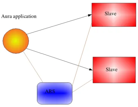
The Aura library supports the parallel rendering on clusters of PCs. The Aura design differs significantly from the Chromium design, at least for two reasons:

1. Aura adopts an ad hoc interface, so it is not transparent to an ap-plication. An application must be rewritten to take advantage of the Aura features, while the intercepting mechanism allows Chromium to be used without modifying the off-the-shelf application. However, the Aura approach permits to optimise the application according to the rendering environment.