Technical Report CoSBi 22/2007
Stochastic Modeling of Budding Yeast Cell
Cycle
Ivan Mura
The Microsoft Research - University of Trento Centre for Computational and Systems Biology
[email protected] Attila Csikasz-Nagy
The Microsoft Research - University of Trento Centre for Computational and Systems Biology
This is the preliminary version of a paper that will appear in Journal of Theoretical Biology
Stochastic Modeling of
Budding Yeast Cell Cycle
Ivan Mura
The Microsoft Research - University of Trento Centre for Computational and Systems Biology
Attila Csikasz-Nagy
The Microsoft Research - University of Trento Centre for Computational and Systems Biology
Abstract
This report presents the definition, solution and validation of a stochastic model of the budding yeast cell cycle, based on Stochastic Petri Nets. A well-established deterministic model, based on ODEs, is considered as the basis for the stochastic modeling. A specific class of Stochastic Petri Nets is selected for building a stochastic version of the deterministic model, with applying the same abstractions of biological phenomena as the ones adopted in the deterministic model. We de-scribe in the report the procedure followed in defining the SPN model from the deterministic one, a procedure that can be largely automated. The validation of the SPN model is conducted with respect to both the results provided by the deterministic one and the results available from wet-lab experiments. A very good match is obtained for the budding yeast wild type and for a variety of mutants that have been experi-mentally constructed in wet-labs. The results of the two models were compared against experimental data. We show that the stochastic-ity allows predicting characteristics that cannot be determined with the deterministic model. Moreover, we also show that the stochastic model can fine-tune the results of the deterministic model, enriching the breadth and the quality of the model.
1
Introduction
Cell cycle is the collective name for a complex network of coordinated bio-chemical phenomena that control the reproduction of the basic living unit, the cell. Cells reproduce by dividing themselves into daughter cells, each one endowed with the biochemical machinery that allows them growing and repeating the process. Before committing themselves to reproduction, cells must grow to an appropriate size, and have to duplicate DNA and segregate the two copies so that each sibling receives one complete copy of it. These tasks are the most delicate ones in the cell cycle, and require the creation of complex structures that ensure each whole copy of the cell genome is first pulled and then confined into a distinct area of the cytoplasm where the daughter nucleus will form.
The cycle of an eukaryotic cell can be split into a sequence of phases, which are common to all organisms. In each phase, specific tasks are accom-plished through the activity of biochemical species, among which cyclin de-pendent kinases (Cdks) play a major role. When bound to a cyclin partner, Cdks are activated and able to make cells to progress along their cycle. Vari-ous Cdks and cyclins exist in eukaryotic cells, and each Cdk/cyclin dimer has specific activity. Changes in the concentration of active Cdk/cyclin dimers are responsible for causing the transition form one phase to the other in the cell cycle. By sensing the internal and environmental conditions through signaling networks, an eukaryotic cell controls the expression of the genes responsible for activation of Cdks, proceeding to the next phase in the cycle only when the current one has been successfully completed.
Higher organisms have a variety of Cdks and cyclins that control the progress of their cell cycle. In the model organism budding yeast Saccha-romices cerevisiae only one Cdk is present (called CDC28), which can com-plex with a limited number of cyclins (CLN1-3 and CLB1-6). Though, the dynamics of the biochemical network controlling the cell cycle of budding yeast follow the same outline as in more complex eukaryotes [4]. Cell cy-cle of buddying yeast has been subject to extensive experimental study and computational models have been developed for it. In particular, the work on deterministic modeling of budding yeast cell cycle conducted by a research team headed by John Tyson at Virginia Tech. has led to the formulation of a comprehensive model, based on ODEs [5]. This model as well as a com-parative analysis of its results and predictions against experimental data are available on the Internet at [1].
In recent years, a number of stochastic modeling techniques started to be applied to model biological phenomena, among which we focus on Stochastic
Petri Nets [11, 19, 20, 14, 15]. This formalism is based on a discrete state-space modeling approach, hence it has the expressive power to capture the discrete molecular dynamics of the system at a lower level of abstraction than deterministic models. When the number of molecules that constitute a molecular network is low, the stochastic modeling may represent a more suitable tool to represent and analyze the dynamics of the system. On the other hand, as the number of molecules grows, abstracting discrete number of molecules into continuous concentration levels and representing evolution of dynamics through a system of coupled ODEs provides very accurate rep-resentations and also has the advantage of not suffering from the state-space explosion problem that plagues stochastic modeling tools.
One of the objectives of this report is to present the definition of a stochastic version, based on SPNs, of an existing deterministic model of budding yeast cell cycle. The deterministic model selected is one produced by Tyson’s research group and described in [9]. The stochastic model is built with a constructive approach that can be largely automated. The second objective of the work we present in the report is the comparative evaluation of the results provided by the models built with the two differ-ent approaches, taking into consideration as well the results obtained with wet-lab experiments. The wild type of budding yeast and various mutants that have been engineered in the lab are considered as the benchmark for the validation of the stochastic model, and for comparing the simulation results provided by the stochastic and the deterministic model. We show that the stochastic model provides results that support the outcome of the deterministic one, and also can be used to probe into more precise analysis of various characteristics of the biological phenomena under consideration. Such analysis, which is based on the probabilistic nature of the stochastic model, cannot be performed with the deterministic model, and are found to better describe results from wet-lab experiments.
The rest of this paper is organized as follows. In Section 2 we describe the cell cycle of buddying yeast, provide some details about the biochemical network that controls its progress through the various phases and present the deterministic model that is used as a basis for the stochastic modeling. Then, in Section 3 we introduce the class of SPNs that are used to build the stochastic model of the system. This stochastic model is defined in Section 4, and Section 5 is devoted to its validation, through the comparison of its result with those provided by the deterministic model and against exper-imental data from wet-lab. Finally, conclusions and directions for future work are given in Section 6.
2
The cell cycle in S. cerevisiae
2.1 Cell cycle narrative descriptionLiving cells reproduce themselves through division into daughter cells. The purpose of cell cycle is to coordinate the replication events necessary to pro-vide the daughter cells with the biochemical cell machinery that is necessary for them to grow and repeat the process. DNA, proteins, RNA, phospho-lipids all need to be more or less duplicated and partitioned between the two cells at division time.
The cell cycle is made up of a precisely coordinated sequence of events whose phasing is mainly controlled by the activity of cyclin-dependent pro-tein kinases (Cdks). The activity level of Cdks determines the progress along the major steps of the cell cycle. For instance, the start of DNA replication, the assembly of the mitotic spindle as well as the condensation of replicated chromosomes, are all events triggered by active Cdks. Cdks get activated when bound with the respective cyclins, and when active are able to regulate (by phosphorylation) many other proteins that trigger the cell cycle events. Most organisms keep the concentration of Cdks to a stable value, and their activity is thus modulated through the variation in the level of cyclins. In higher eukaryotic organisms, many Cdks and cyclins made up a network of molecular signals, but it has been found that the same basic mechanisms of cell cycle control are accomplished in simpler organisms through a limited number of biochemical species. The budding yeast is a well-studied and understood example of how the cell cycle can be controlled with only one Cdk and a few cyclins [4].
The cell cycle of eukaryotes can be divided in four major phases, namely G1, S, G2, M, where G1 and G2 are two gap phases, S is the synthesis phase (DNA duplication) and M is the mitosis phase:
G1 : gap phase G1 takes place right after a cell division. The cell is uncom-mitted to the replication phase process. By sensing the environment conditions, and after reaching an adequate mass, a cell can commit itself to start the next phase, a cell cycle transition called Start.
S : in this phase the cell duplicates its genetic material. Once the process is started at the beginning of the synthesis phase, it goes irreversibly to completion.
G2 : in gap phase G2 the cell checks again that the environment is favorable to proceed to the next phase and ensures the duplication of DNA has
completed. If any problems occurred in such duplication, the cell arrests the cycle in this phase until the problem is solved.
M : the mitosis phase is divided in various subphases. During the prophase, chromatin in the nucleus begins to condense into chromosomes. Cen-trioles begin moving to opposite ends of the cell and microtubule fibers extend from the centromeres. In the prometaphase proteins attach to the centromeres creating the kinetochores. Microtubules search for the kinetochores and once found them, the chromosomes begin mov-ing. During the metaphase, spindle fibers align the chromosomes along the middle of the cell nucleus. At this point, a second irreversible transition happens, which commits the cell to proceed in the mito-sis. When all chromosomes are properly aligned, the cell passes the so called Spindle checkpoint event, and proceeds into the anaphase, during which the daughter chromosomes separate pulled at the kine-tochores and move to opposite sides of the cell. During telophase, chromatids arrive at opposite poles of the nucleus, and the partition-ing of the cell is performed, through the contraction of the actin fibers that cause an elongation of the cytoplasm and ultimately the division of the cell.
The phases described above are triggered by the active Cdks, and are additionally controlled by signaling networks that are able to sense the en-vironment conditions and the completion of the various processes of DNA replication, condensation and chromosome alignment. We shall focus here-after on the biochemical machinery that controls Cdks activity in budding yeast, as described in [9].
In budding yeast, during the G1 phase, the activity of Cdk1 (the only budding yeast Cdk, also called Cdc28) is low because the cyclin mRNA transcription is mostly inhibited. Moreover, the produced cyclin proteins are rapidly degraded by the activity of a set of proteins collectively called anaphase-promoting complex (APC). The APC consists of several polypep-tides and two auxiliary proteins, Cdc20 and Cdh1. When active, these two latter proteins mediate the presentation of various targets (including cyclin) to the APC for labeling through multi-ubiquitin chains. Ubiquitylated tar-gets are quickly degraded in proteasomes. In G1 phase, there is abundance of active Cdh1. Furthermore, during G1 the remaining Cdk1/cyclin dimers are sequestered by a stoichiometric inhibitor (CKI - Sic1), which forms with Cdh1/cyclin dimers an inactive heterotrimer.
If the environmental conditions are favorable, as the cell progresses in the G1 phase the mass of cell grows, and this leads to an increased
produc-tion of a transcripproduc-tion factor (TF - SBF/MBF) that activates genes for the production of the starter kinase (SK - Cln’s). SK has the effect of mediating the degradation of both Cdh1 and CKI, which allows mitotic cyclins (Clb’s) to start accumulating in the cell. This change in the biochemical dynamics of the cell corresponds to the Start event, and the beginning of the S phase. Cyclin synthesis in induced and cyclin degradation inhibited throughout S, G2, and M phases. The active Cdk/cyclin complexes drive the cell through the various stages of the synthesis and mitosis phase. A further increase in Cdk activity at the Start transition is caused by the ability of the Cdk/cyclin dimers to phosphorylate CKI molecules. Such phosphorylation labels CKI molecules for degradation by the proteolytic cell machinery, increasing the amount of active Cdk/CycB dimers. Such high concentration of active Cdk also has the effect of causing the degradation of the TF for the starter kinase SK, which has already accomplished its role in the cell cycle.
Upon entering into the S phase, the Cdc20 protein starts to be synthe-sized. This synthesis is again driven by the activity of the active Cdk/cyclin. At the metaphase/anaphase transition, Cdc20 molecules bind at the APC and activate it through a signal generated by the mitotic process itself, sup-posedly thorough intermediate enzymes (IE). The active Cdc20 causes the degradation of the cyclin CycB and activates the other APC protein, Cdh1. This change in the biochemical activity of the APC regulator proteins cor-responds to the Finish transition. The activity of the two APC proteins Cdc20 and Cdh1 leads the cell into the anaphase of mitosis. Moreover, their combined activity leads to a quick degradation of the available cyclins. This inactivation is the primary responsible for the disassembly of the spindle. As the Cdk activity reverts to low level, the telophase completes and the cell divides. The synthesis of the APC related protein Cdc20 stops as the activity of Cdk is lost, and the newborn cell enters the G1 phase.
2.2 Cell cycle deterministic mathematical model
We shall describe in this section the deterministic model proposed in [9] for capturing the biochemical dynamics of the cell cycle in budding yeast. The picture in Figure 1 is a slightly revised one from that shown in [9], on page 270. It shows the biochemical species involved in the cell cycle, and depicts the main reactions. Dashed lines represent the mediation effect that some species have on reactions.
It is worthwhile observing that the Cdks are not included in the model, as their concentration is assumed to be constant throughout the cell cycle and in excess with respect to the available cyclin partners. Moreover, the
Figure 1: Graphical representation of cell cycle engine
model also assumes that the concentration of Cdk/CycB dimers (the active Cdks) is always in equilibrium with the CycB and Cdk concentration, and the same is assumed for the CKI/Cdk/CycB trimers.
The following system of ordinary differential equations (ODEs), pro-posed in [9] on page 271, provides a deterministic model for the biochemical processes described in Figure 1.
dm dt = µm(1 − m/m ∗) (1) d[CycBT] dt = k1− (k ′ 2+ k ′′ 2[Cdh1A] + k ′′′ 2 [Cdc20A])[CycBT] (2) d[Cdh1A] dt = (k3′+ k ′′ 3[Cdc20A])(1 − [Cdh1A]) J3+ 1 − [Cdh1A] − (k4m[CycB] + k ′ 4[SK])[Cdh1A] J4+ [Cdh1A] (3) d[Cdc20T] dt = k ′ 5+ k5′′ (m[CycB])n Jn 5 + (m[CycB]) n− k6[Cdc20T] (4) d[Cdc20A] dt = k7[IEP ]([Cdc20T] − [Cdc20A]) J7+ [Cdc20T] − [Cdc20A] − k8[Cdc20A] J8+ [Cdc20A]− k 6[Cdc20A] (5) d[IEP ]
dt = k9m[CycB](1 − [IEP ]) − k10[IEP ] (6)
d[CKIT] dt = k11− (k ′ 12+ k ′′ 12[SK] + k ′′′ 12m[CycB])[CKIT] (7) d[SK] dt = k ′ 13+ k ′′ 13[T F ] − k14[SK] (8) d[T F ] dt = (k15′ m + k ′′ 15[SK])(1 − [T F ]) J15+ 1 − [T F ] − (k′16+ k ′′ 16m[CycB])[T F ] J16+ [T F ] (9)
In the equations above, [X] indicates the concentration of biochemi-cal species X. [CycBT] indicates the total concentration of cyclin CycB
(Cdk/Clb complexes), including the one that is bound in the Cdk/CycB dimers and the one bound in the CKI/Cdk/CycB trimers. Similarly, [CKIT]
denotes the total concentration of the free CKI (Sic1) plus that of the CKI bound in the trimer. Because it is assumed that the concentration of Cdk/CycB dimers and CKI/Cdk/CycB trimers is always in equilibrium with the concentrations of CKI, Cdk and CycB, we can obtain the concen-tration of the dimers, which is denoted in the model by [CycB], as a function of [CycBT] and [CKIT], as follows:
[CycB] = [CycBT] − [T rimer] = [CycBT] −
2[CycBT][CKIT]
Σ +pΣ2
− 4[C ycBT][CKIT]
(10)
where Σ = [CycBT] + [CKIT] + Keq−1. Equation (1) models cellular growth.
Several terms in the other equations are dependent on the cell mass, to model the dependence that the dynamics of the system has on cell size. Notice that this systems of ODEs is not including a mathematical formulation of the cell division. This event is added to the model as an external action, in a way that the cell mass is halved when the concentration of active Cdk/CycB falls below an assigned threshold (0.1, in this model) during telophase (this is a simplification of the asymmetric division of budding yeast cells). The ODE model is completed with a set of values for the rate constants, which are not
reported here for the sake of conciseness. The interested reader can obtain them from [9] on page 273.
It is important to notice the different levels of abstraction at which the various reactions are modeled. For instance, the last term in equation (4) models the degradation of Cdc20, and is easily recognized as the determin-istic model of a first order reaction. In that same equation, the second term in modeling in quite an abstract way (by the so-called Hill function) the dependence of Cdc20 production on cell mass and [CycB]. This vari-able level of abstraction has important implications on the selection of the modeling formalism that can be applied to define a stochastic model of this same biological system. Indeed, the deterministic model will be much easier translated into a modeling formalism that allows representing those same different levels of abstraction therein adopted.
3
Stochastic Petri nets modeling formalism
In this section we shall present the stochastic Petri net formalism that we adopt as the tool to build a stochastic cell cycle model. Many variants of modeling notations exist for SPNs (a comprehensive list can be found at the web site [2] maintained by the University of Hamburg), therefore we shall first describe in this section the precise notation we will be using, to make sure that no ambiguities exist in the interpretation of the models. Various families of SPNs exist that match the features of the modeling formalism described in this section, e.g., [7, 6]. Before entering into the details of the modeled examples we shall also briefly recall the classical interpretation of Petri net modeling elements in biology.
We shall use the basic elements of Petri nets, i.e. places, transitions, arcs and tokens with following the standard graphical notation reported in Figure 2. The rules to compose correct SPN models from the basic modeling
Figure 2: Basic Petri net modeling elements
elements are the following ones:
• arcs can only connect a place to a transitions or a transition to a place, i.e., the graph that represents the structure of the net is a bipartite one.
The number of tokens inside a place defines the marking of the place. The marking of the Petri net model is the vector that collects all the markings of the places in the model. A transition is said to be enabled if each of its input places, i.e. the places from which an arc exists going from the place to the transition, contain at least one token. An enabled transition fires in a random time. We shall stick to a limited set of distributions of the random variables representing the firing time:
• the negative exponential, completely described by a single parameter λ, called the rate;
• the deterministic distribution with constant firing time equal to 0 (transitions with such firing time distribution are depicted as thin bars and called instantaneous transitions).
We shall allow transition having rates whose value are mathematically expressed through arbitrary functions of the model marking. Hence, every exponential transition ti of the model will have associated a rate function
ri(·) : Nh → R, where h is the number of places in the model. For every
marking of the net ~n, ~n ∈ Nh, the value of rate function r
i(~n) returns the
rate of the exponential distribution that models the occurrence time of the event represented by the transition.
Furthermore, the enabling of transitions can be controlled through as-sociated guards, i.e., logic predicates that are defined as marking-dependent functions. Guards provide a very compact way of modeling complex condi-tions that apply on the occurrence of events.
The firing of a transition atomically removes one token from each input place of the transition and deposits one token in each of the output places of the transition, i.e. those places for which an arc exists going from the transi-tion to the place. Conflicts among enabled transitransi-tions, i.e. those situatransi-tions in which multiple transitions are enabled and these transitions share some input places, are resolved by using a race policy, i.e. the shortest random time among those of all enabled transitions is the one that determines which transition will fire. After the firing, the marking of the net is changed, a new set of transitions may be enabled for firing and if conflict still exist, a new race will occur. If an enabled transition gets disabled from a conflicting one, the memory of the elapsed time it has been enabled is lost, and at the next
enabling a new random firing time will be sampled from the negative expo-nential distribution of the transition. However, notice that this rule, albeit useful for understanding the rules of concurrent firing, is unessential because of the memoryless property of the negative exponential distributions.
Moreover, we allow arcs having assigned positive integer weights func-tions, (defaulted to the constant function 1, not indicated) which enrich the possibility of controlling the token flow after transition firing. Weight func-tions on arcs can be defined as marking-dependent funcfunc-tions. A transition will be enabled if all the input places contain at least as many tokens as the current weight of the connecting arc. When a transition fires, it removes from each input place as many tokens as the weight of the connecting arc, and puts as many tokens as the weight of the connecting arc inside each output place.
Being an abstract modeling formalism, Petri nets by themselves do not refer to any specific aspect of the biological domain, but rather a meaning has to be associated by to modeler to places, tokens and transitions. In the context of biological phenomena, the classical interpretation of Petri net elements is the following one:
• Places represent chemical species or more complex biological entities as well, such as as ribosomes, receptors, genes.
• Tokens inside a place (the marking of the place) model the number of molecules of the species or of the entity represented by the place. Notice that tokens are anonymous entities that do not carry any qual-ifying information, and thus the molecule or the biological entity they represent changes as they move from a place to another1
. Notice that tokens are not always graphically depicted, apart from the cases in which there are a few of them, but rather they are associated to places when providing the initial state of the models.
• Transitions represent biochemical reactions. The exponential rate as-sociated to a transition expresses the speed at which a reaction oc-curs. The infinite server semantics of the firing is the one commonly adopted, meaning that, if the number of tokens in the input places allows for multiple reactions to proceed concurrently, the rate of the reaction is multiplied by the number of the reactions, which is indeed quite a simple way of modeling chemical reactions obeying the mass-action law.
1
Some Petri net modeling formalisms (for instance Colored Petri Nets [12]) allow for tokens having attributes
4
SPN modeling of S. cerevisiae cell cycle
In this section, we shall use the Stochastic Petri Nets formalism described above to define a stochastic version of the cell cycle deterministic model described in Section 2.2. The SPN model has one place for each of the biochemical species considered in the deterministic model, and one transition for each possible reaction. The complete SPN model for the cell cycle, which we obtained with the constructive approach defined below, is shown in Figure 3.
Figure 3: SPN model of budding yeast cell cycle
Let us consider for instance the ordinary differential equation (3). This equation is describing the time-dependent evolution of the concentration of active molecules of species Cdh1. Therefore, the SPN model will have one place, named Cdh1A, containing tokens that represent the active molecules
of Cdh1, and one place named Cdh1 containing tokens that represent the inactive molecules of Cdh1. Differential equation (3) is describing 4 possi-ble reactions; out of them, 2 transform inactive molecules into active ones, and 2 model the opposite transformation. Hence, the SPN model will have four reactions that move tokens between the Cdh1A and the Cdh1 places.
The first reaction in equation (3) is occurring with a rate constant given by k3′(1 − [Cdh1A])/(J3+ 1 − [Cdh1A]). Notice that 1 − [Cdh1A] is
equiv-alent to [Cdh1] because there is neither creation nor degradation of Cdh1 molecules. Therefore, in the deterministic model this transformation is mod-eled through a first order reaction that only depends on the concentration of the inactive Cdh1 through the mass-action law. A transition t5 is included
in the SPN to model this reaction, and its rate function is defined as follows:
r5(#Cdh1) =
k′3#Cdh1
J3+ α#Cdh1
(11)
where #X denotes the number of tokens contained in place X and α is a constant scaling factor that accounts for mapping a concentration into an equivalent number of molecules, for a given volume in which the reaction takes place [10].
Let us now consider the second term in equation (3), whose rate constant in the deterministic model is given by k3′′[Cdc20A](1 − [Cdh1A])/(J3+ 1 −
[Cdh1A]), or equivalently, k
′′
3[Cdc20A][Cdh1]/(J3+ [Cdh1]). This expression
tells that the a reaction of activation exists for Cdh1, which is driven by the active molecules of species Cdc20. A transition t6 is included in the SPN
model to represent this reaction, and its firing rate is defined as follows:
r6(#Cdc20A, #Cdh1) =
k3′′α#Cdc20A#Cdh1
J3+ α#Cdh1
(12)
Similarly, we can model all the reactions that are described in the de-terministic model provided by the differential equation (2),(3),. . . ,(9). It is important to remark the fact that such a simple one-to-one translation, from the terms of the differential equations into the transitions of the stochastic model, is made possible because of the expressive power of the specific class of selected SPNs. The possibility of defining general rate functions of transi-tions allows building a stochastic model at an analogous level of abstraction as the one adopted in the deterministic one.
Translating equation (1) into the stochastic model requires a different process. Indeed, that equation does not have a discrete counterpart in terms of a discrete number of molecules. Therefore, it is included in the SPN model with a transition growth whose firings represent an increase in the mass of the cell. The mass itself is represented by the number of tokens contained in place M ass. The condition for which the cell divides has to occur is a marking-dependent guard assigned to transition division. When the condition is satisfied, division fires immediately, and its firing removes all the tokens contained in place mass (through a marking-dependent weight on the connecting arc) and puts half of them back into mass (through another
marking-dependent arc). In the SPN model in Figure 3, we denoted arcs having associated marking-dependent weights as having a small mark along them (see the arcs connecting transition division to M ass place).
The specification of the SPN model is to be completed with all the rate functions of transitions, the weight functions of arcs and the guards added to transitions to control their enabling. As we have already described in detail how the rates are obtained from the terms of the ODEs composing the deterministic model, and presented the specific aspects of the modeling for the equation ruling mass evolution, we omit this part of SPN definition. The SPN model has been implemented into one tool that supports the adopted modeling formalism, i.e., the M¨obius tool [7], which allows for graphical model definition and for solution via simulation.
5
Stochastic model validation
In this section we shall present the result of SPN model solution and will compare them with the results provided by the deterministic model and with those obtained via wet experiments with the purpose of validating the stochastic version. To this, we solve the SPN model (via simulation) and the system of ODEs (numerical integration) for the wild type budding yeast and for a set of mutants that can be easily modeled with simple changes to the two models. A vast repertoire of budding yeast mutant strains has been generated in the lab, by deletion of the genes that code for some of the proteins involved in the cell cycle. The results of such experimental work is described in detail in the budding yeast cell cycle Internet page [1].
5.1 Wild type
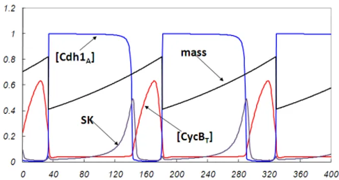
We compare in this section the results provided by the SPN model and the deterministic one for the wild type of budding yeast. We show in Figure 4 the curves for the time courses of the cell mass, the total concentration of cyclin [CycBT] and the concentration of the active form of APC protein activator
[Cdh1A], as obtained from the system of ODEs defining the deterministic
model. The WPP software (available for download on [3]) has been used for numerical integration over the time interval [0-400] (time unit is minute).
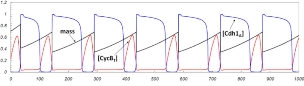
The results obtained from the simulation of the SPN model for an anal-ogous interval [0-400] of simulated time are shown in Figure 5. For visual purposes the protein numbers have been rescaled to concentrations for all plots. The model simulation was performed with the M¨obius tool [7]. A single run of simulation results is shown in Figure 5, which was started
Figure 4: Deterministic model results for the wild type
with the same initial state as the one applied to the ODE system of equa-tions. The simulation was repeated mutiple times with different seeds of the pseudo-random number generator, and the only difference among runs was the stochastic fluctuation in cell cycle duration, also appreciable in Figure 5 for the single run.
Figure 5: Stochastic model results for the wild type
We conducted a simulation experiment consisting of 1000 runs, each using a disjoint sequence of pseudo-random numbers, to evaluate the average cycle time duration and the average mass at cell division time in the SPN model. We compare the obtained result against the value obtained from the deterministic model in Figure 6. For the results computed through the simulation of the SPN model, Figure 6 also shows the confidence interval computed from the observations. The confidence intervals were computed at the 95% level of confidence. For both results, the relative width of the confidence interval is less than 1%. As it can be observed, there is a close
match between the results of the two models, and the ODE results falls within the confidence interval obtained via simulation.
Figure 6: Comparison of cycle time and mass statistics
5.2 Mutant with SK deleted - cln1∆, cln2∆, cln3∆
Let us now consider the mutant of budding yeast that is obtained with inhibiting the production of the all the starter kinases - SK in the model. Because in our models SK is responsible for starting the series of biochemical processes that let the cell to Start event and enter into the S phase, we expect the mutants cell not to be able to start DNA duplication and block in G1 phase.
Allowing for such a mutation in the ODE and SPN models is quite straightforward: simply setting to 0 a few parameters and appropriately changing the initial conditions leads to the definition of the model of the mutant.
We show in Figure 7 a [0-400] minutes time course as computed by solving the deterministic model. As expected, the mutant is not viable.It is indeed able to complete mitosis once, because the initial condition sets the state of the model after the S phase, when the SK has already accomplished its role and it is not necessary anymore. However, in the subsequent cell cycle, the lack of SK blocks the mutant into G1, as nothing can inhibit the accumulation of the Cdk/CycB stoichiometric inhibitor CKI and of the active Cdh1. Consequently, the total concentration of CycB stays very low and what is available in the cell is bound with CKI and thus inactive, the typical condition of the G1 phase.
Figure 8 shows one time course over [0-400] minutes for the SK deleted mutant, as obtained from a single simulation run of the stochastic model.
Figure 7: Deterministic model results for the SK deleted mutant
Figure 8: Stochastic model results for the SK deleted mutant
The match with the result provided by the deterministic one is very accurate. The first mitosis is completed and then the cell blocks in G1. Additional runs of simulation performed using different sequences of pseudo-random numbers provided exactly the same chart.
These simulation outcomes match the experimental result that this mu-tant is not viable as it arrests in G1 phase [16].
5.3 Mutant with Cdc20 deleted - cdc20∆
This mutation removes the APC mediator Cdc20 from the cell. Because Cdc20 activity is responsible for the activation of the APC at the metaphase to anaphase transition (Finish), the mutant is not to be able to complete mitosis and blocks in the metaphase [18]. The results of the deterministic
model shown in Figure 9 match this observation.
Figure 9: Deterministic model results for the Cdc20 deleted mutant
The same result is obtained with simulation ofr the SPN model, as shown in Figure 10.
Figure 10: Stochastic model results for the Cdc20 deleted mutant
5.4 Mutant with SK and CKI deleted - cln1∆, cln2∆, cln3∆, sic1∆
Because one of the main consequences of SK activity is to cause the degra-dation of the Cdk/CycB stoichiometric inhibitor CKI, it is interesting to look at a double mutant in which both SK and CKI are deleted. Indeed, in this case it is not obvious whether the cell would stop in G1 phase, or the active CycB cyclin may raise to a level that overrides the activity of Cdh1 and enter into S phase.
We show in Figure 11 a [0-1000] minutes time course of model results, as provided by the ODE model. The ODE model shows the viability of this double mutant, which matches the experimental observations [21].
Figure 11: Deterministic model results for the SK and CKI deleted mutant
Figure 12 shows the results obtained with one simulation run of the SPN model, over a time window of [0-1000] minutes of simulated time. The results of the stochastic model also suggest the viability of this double mutant, with an appreciable increase in the variability of the cell cycle duration.
Figure 12: Stochastic model results for the SK and CKI deleted mutant
5.5 Mutant with CKI deleted - sic1∆
In this section we consider the mutant deprived of the stoichiometric in-hibitor of the Cdk, modeled by species CKI.
We shown in Figure 13 the results provided by the deterministic model of the mutant, over a [0-1000] minutes time window. The ODE results shows the viability of the mutant, which fits the experimental observations [17].
The simulation output of the SPN model resembles the results of the deterministic one, as it can be observed from Figure 14. It can be observed
Figure 13: Deterministic model results for the CKI deleted mutant
from the simulated time course that the cell cycle in this mutant shows rele-vant irregularities, with high variability in its length. Moreover, the mutant appears to have problems in degrading CycB, which leads to a prolonged M phase. On the other hand, some other cycles show a very regular pattern of oscillations, perfectly matching the one returned by the deterministic model in Figure 13. It is important to mention that delayed cell cycles have been experimentally observed for this mutant, giving a nick name to sic1∆ cells as ”sick” cells [13].
Figure 14: Stochastic model results for the CKI deleted mutant
We conducted a simulation experiments to compute a few statistics for the cell cycle of CKI deleted cells. We computed first of all the average values of cell cycle duration and of the cell mass, and compared them against the deterministic results provided by the ODEs, as shown in Figure 15. Steady state simulation (1000 runs) was used to compute the statistics, with 95% confidence level of results. As it can be observed, the results provided by the two models are in agreement at this level.
Then, we looked at the spread of the observations. We plot in Figure 16 the relative frequencies of occurrence of the cycle time durations over a time interval [80-200] minutes, for CKI deleted mutant and for the wild type cell simulations. As it can be observed, the cycle time duration of the mu-tant exhibits a much higher variability, in agreement with the experimental observations [13]. Thus, the stochastic model could reveals the ”sick” non
Figure 15: Comparison of deterministic and stochastic average values
robust cell cycles of sic1∆ cells.
Figure 16: Distribution of cell cycle time for wild type and mutant
5.6 Mutant with Clb2 destruction box deleted and Clb5 deleted - Clb2db∆, clb5∆
We consider in this section the mutant obtained with the deletion of the de-struction box of cyclin Clb2 (which mutation reduces its degradation rates), and with the deletion of cyclin Clb5 (which reduces the overall CycB level). These two cyclins are collectively modeled by species CycB, both in the ODE
and in the SPN model. We can represent these two mutations as follows: • the deletion of cyclin Clb2 destruction box is modeled by removing the
activity of active Cdc20 to degrade CycB and by reducing the degra-dation rate of CycB by active Cdh1 (residual Cdh1 activity remains because of the KEN box on Clb2) [22];
• the deletion of cyclin Clb5 is modeled by reducing the production rate of CycB.
Experimental results show that this mutant is viable, but only under those circumstances that slow down its growth rate [8]. This is the case, for instance, when the mutant uses galactose as a source of energy. There-fore, to simulate the growth in the galactose medium, we reduce the rate constant of growth speed from 0.005 (the default value in all of the other models, supposed the cells grow on glucose there) to 0.004. The determin-istic model results for such mutant are shown in Figure 17, and correctly show its viability.
Figure 17: Deterministic model results for the Clb2 destruction box deleted and Clb5 deleted mutant
Figure 18 shows the results obtained from the SPN model of the mutant. As it can be observed, the time courses returned by the two models match very well.
It is interesting to observe that the deterministic model is able to fit the lethality of the mutation in glucose (growth rate µH=0.005) and its
viability in galactose (growth rate µL ≈ 0.0041) but cannot predict the
intermediate situations. It is reasonable to expect a continuous transitions as the growth rate varies in the interval [µL− µL], with some mutant cells
having a limited survivability for values of the growth rate inside the interval. If in population of mutant cells each of them are able to complete, with a certain probability, a sufficient number of cells cycles before dying, a colony
Figure 18: Stochastic model results for the CKI deleted mutant
may develop, even if its overall growth would be slow. Such small colonies have been experimentally observed for various types of mutants.
We show in Figure 19 the results provided by the stochastic model for a run using the growth rate value µ = 0.0047, in which the cell was able to complete two cycles before reaching a state that does not allow it to survive further.
Figure 19: A mutant cell completing two cell cycles before dying
We conducted an in-silico experiment to evaluate the probability that a single mutant cell would be able to divide at least 10 times before dying (forming a small colony), with varying the growth rate within the interval [µL− µL]. The results of the simulation are shown in the chart in Figure
20, together with their confidence intervals. Also, that same probability is shown for the result provided ODE, obvioulsy jumping from zero to one as the critical value µL is reached. For each value of the growth rate, we run
100 batches, each one using different a different sequence of pseudo-random numbers.
The results in Figure 20 clearly show that colonies of the mutant may exist for values of the growth rate higher than the threshold value µL, which
Figure 20: Probability of having at least 10 replications of a mutant
Thus we present that stochastic simulations can be important to check the ”partial” viability of some mutants that are at the border of life and death.
6
Conclusions and future work
This report presents the results of a modeling activity for the cell cycle of budding yeast cells. A well established deterministic model, based on ODEs, has been taken as the starting point for constructing an SPN model of the cell cycle biochemical machinery. The SPN model was built with adopting the same abstraction level captured by the deterministic model. A simple and largely automatable procedure for mapping ODEs into SPN constructs has been presented through its application to the process of model definition. The resulting SPN model has been described, and then its validation conducted, with a comparison of the results obtained via simulation against the results provided by the deterministic model as well as with reference to experimental results. The validation encompassed the wild type and various mutants of budding yeast.
The validation showed a general agreement between the results of the two models. We demonstrated how the stochastic version of the model can however provide deeper insights about the cell cycle of the modeled organisms, as it allows a statistic characterization of cell cycle parameters such as duration and average cellular mass, and also provides a more precise solution in some circumstances under which the viability of mutant cells is probabilistic and cells may die after completing a few cell cycles.
More detailed deterministic models of the cell cycle in budding yeast are available in the literature, which include molecules other than the ones
we considered in this report. In our future work we plan to extend the stochastic modeling by looking at the information contained in these mod-els, starting with the model in [5]. Furthermore, we can enrich the model with the explicit modeling of the various checkpoints. These checkpoints are controlled by a number of signaling pathways that ensure the completion of various step of the cell cycle, such as DNA replication, complete formation of the mitotic spindle, alignment of chromosomes. Hence, the explicit mod-eling of checkpoints provides the interface points in the cell cycle to include detailed models of those pathways, an activity that we shall tackle in our future work.
References
[1] http://mpf.biol.vt.edu/research/budding yeast model/pp/index.php. [2] http://www.informatik.uni-hamburg.de/tgi/petrinets.
[3] http://www.math.pitt.edu/ bard/xpp/download.html.
[4] B. Alberts, A. Johnson, J. Lewis, M. Raff, K. Roberts, and P. Walter. The cell. Garland Sciences, 2002.
[5] K. C. Chen, L. Calzone, A. Csikasz-Nagy, F. R. Cross, B. Novak, and J. J. Tyson. Integrative analysis of cell cycle control in budding yeast. Molecular biology of the cell, 15(8):3841–3862, 2004.
[6] G. Ciardo, J. K. Muppala, and K. S. Trivedi. SPNP: Stochastic petri net package. In International Workshop on Petri Nets and Performance Models (PNPM’89), pages 142–151, 1989.
[7] G. Clark, T. Courtney, D. Daly, D. Deavours, S. Derisavi, J. M. Doyle, W. H. Sanders, and P. Webster. The M¨obius modeling tool. In Interna-tional Workshop on Petri Nets and Performance Models (PNPM’01), pages 241–250, Los Alamitos, CA, USA, 2001. IEEE Computer Society. [8] F. R. Cross. Two redundant oscillatory mechanisms in the yeast cell
cycle. Developmental Cell, 4:741–752, May 2003.
[9] C. P. Fall, E. S. Marland, J. M. Wagner, and J. J. Tyson, editors. Computational Cell Biology. Springer-Verlag, 2002.
[10] D. Gillespie. Exact stochastic simulation of coupled chemical reactions. The Journal of Physical Chemistry, 81(25):2340–2361, 1977.
[11] P. J. E. Goss and J. Peccoud. Quantitative modeling of stochastic systems in molecular biology by using stochastic Petri nets. Proceedings of the The National Academy of Sciences, 95(12):6750–6755, June 1998. [12] K. Jensen. An introduction to the practical use of coloured petri nets. In W. Reisig and G. Rozenberg, editors, Lectures on Petri Nets II: Applications, volume 1492 of Lecture Notes in Computer Science, pages 237–292. Springer-Verlag, 1998.
[13] T. T. Nugroho and M. D. Mendenhall. An inhibitor of yeast cyclin-dependent protein kinase plays an important role in ensuring the ge-nomic integrity of daughter cells. Molecular biology of the cell, 14:3320– 3328, 1994.
[14] T. Nutsch, D. Oesterhelt, E. D. Gilles, and W. Marwan. A quantitative model of the switch cycle of an archaeal flagellar motor and its sensory control. Biophysical Journal, 89(4):2307–2323, October 2005.
[15] M. Peleg, D. Rubin, and R. B. Altman. Using Petri net tools to study properties and dynamics of biological systems. Journal of the American Medical Informatics Association, 12(2):181–199, 2005.
[16] H. Richardson, C. Wittenberg, F. R. Cross, and S. I. Reed. An essential G1 function for cyclin-like proteins in yeast. Cell, 59:1127–1133, 1989. [17] B. L. Schneider, Q.-H. Yang, and A. B. Futcher. Linkage of replication
to Start by the Cdk inhibitor Sic1. Science, 272:560–562, 1996.
[18] N. Sethi, M. C. Monteagudo, E. Hogan, and D. J. Burke. The CDC20 gene product of Saccharomyces cerevisiae, a beta-transducin homolog, is required for a subset of microtubule-dependent cellular processes. Molecular biology of the cell, 11:5592–5602, 1991.
[19] R. Srivastava, M. S. Peterson, and W. E. Bentley. Stochastic kinetic analysis of Escherichia coli stress circuit using σ32 targeted antisense.
Biotechnology & Bioengineering, 75(1):120–129, October 2001.
[20] D. Tsavachidou and M. N. Liebman. Modeling and simulation of path-ways in menopause. Journal of the American Medical Informatics As-sociation, 9(5):461–471, 2002.
[21] M. Tyers. The cyclin-dependent kinase inhibitor p40sic1 imposes the requirement for Cln G1 cyclin function at Start. Proceedings of the The National Academy of Sciences, 93:7772–7776, 1996.
[22] R. Wasch and F. Cross. APC-dependent proteolysis of the mitotic cyclin Clb2 is essential for mitotic exit. Nature, 418:556–562, 2002.