VEHICULAR TRAFFIC SIMULATIONS:
USE OF A GAMES ENGINE FOR VIDEO
RENDERING AND VERIFICATION
OF AN ARCHITECTURE MODEL BASED
ON QUEUING SYSTEMS
LEONARDO PASINI, FRANCESCO MARIA RIETTI
AND
FABRIZIO ALLEGRETTO
Department of Computer Science, University of Camerino Via del Bastione 1, Camerino, Italy
(received: 15 April 2016; revised: 16 May 2016; accepted: 23 May 2016; published online: 1 July 2016)
Abstract: In a previous work [Pasini L and Sabatini S 2016 TASK Quart. 20 (1) 9], we described a technique that allows a specific system of urban traffic to be associated to a description file system, called Model.dat. This file contains a list of data objects that are defined in the library [Pasini L and Feliziani S 2013 TASK Quart. 17 (3) 155] and that form the architecture model of a vehicular traffic system. This model turns out to be a network of queuing systems. In this work, we illustrate how we adapted the old procedure to study a new urban traffic system. Moreover, through a new tracking procedure, we illustrate how we developed a graphic simulation able to reinterpret the data from the simulation of the queuing networks model, in order to make it easier to check the effectiveness of the simulator and to have a graphical way to analyze the data.
Keywords: traffic systems, queuing networks, modelling and simulation, graphic simulation
1. Introduction
In this paper, we explain the work done in a study developed to produce a simulation of a new urban vehicular traffic system. The aim of the study is to keep track of what happens during the simulation to allow the creation of a graphic simulator. To achieve this, we took a technique explained previously [1] where we described how to allow a specific urban traffic system to be associated to a description file system, and we made some substantial changes to achieve our goal. Firstly, we changed the CreaModeldat.xls files to make them fit to the new road system, allowing the correct generation of Model.dat files, essential for the simulation of the queuing networks model corresponding to the vehicular
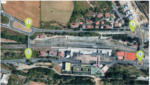
model analyzed by simulation is a road network composed of four roundabouts, with corresponding connecting roads.
Figure 1. System View
Each roundabout is marked by a number: the first one is placed to the North West of the system, the second to the South West, the third to the North East and finally, the fourth roundabout to the South East. All four are connected between one another by several streets, in particular:
• Ponte Nuovo, which connects the first and the second roundabouts; • Via Lombardi, which connects the first and the third roundabouts; • Via Mazzini, which connects the second and the fourth roundabouts; • Ponte Malizia, which connects the third and the fourth roundabouts; The pathways that allow the output from the considered system are: • Via Bandinelli and Via Giovanni Paolo II, which allow exiting the system
through roundabout 1;
• Via Sclavo, which allows exiting the system through roundabout 2; • Via Bracci and Via Grondaie, for roundabout 3;
3. Roundabout Components
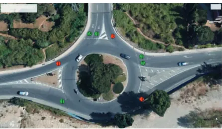
After a detailed study of the system, many components were identified for each roundabout, including in particular:
• Road: which can be internal or external to the system, and it is indicated by a solid blue line in the graphical representation;
• Flows: it allows generating vehicles that will enter the system, and it is indicated by an orange rectangular shape;
• Road Multiplexer: it allows the traffic to be divided on routes and it is indicated with a green triangle;
• Input Section: it is the entry to a roundabout and it is represented by a green circle;
• Output Section: it is the output from a roundabout and it is indicated by a red circle;
• Simple Multiplexer: it divides the traffic across a multiple input section, or simply inputs;
• Path: it represents a possible path from any input of a roundabout to an output of the same;
• Arc: it indicates a portion of the road, one or more arcs together can compose a path.
The process of our modelling work concerning the four Roundabouts will be shown below.
3.1. North-West Roundabout
The first roundabout, located to the North-West of the examined system, allows inflows and outflows of vehicles from two streets outside the system (Via Bandinelli and Via Giovanni Paolo II) and from two streets inside it (Ponte Nuovo and Via Lombardi). Coming out of the first roundabout, drivers will have two possibilities: (1) they will be able to reach the second roundabout, continuing on Via Ponte Nuovo; (2) or they will be able to reach the third roundabout, continuing on Via Lombardi (Figure 2).
The picture shows that all entries and exits from this roundabout as well as external and internal streets to the system are single-lane.
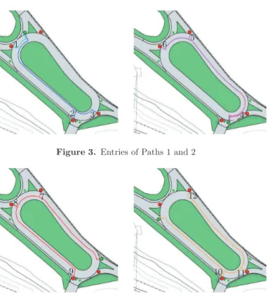
In Figures 3 and 4, all possible paths for each roundabout entrance are indicated. Remembering that a path is a route from an entry to an exit of a roundabout and that each path is composed of a given number of arcs, in the graphical representation, the input (green color), from which different paths will start, and output sections (red), in which paths will end, will be indicated with a black border.
The North-West roundabout model is made up of several objects which are shown in the Figure 5.
3.2. South-West Roundabout
The second roundabout, located to the South-West of the examined system, allows the inflow and outflow of vehicles from a street outside the system (Via
Figure 2. North-West Roundabout
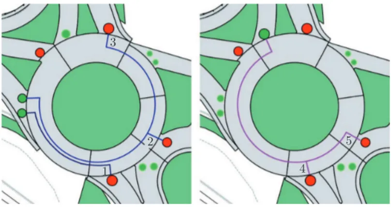
Figure 3. Entries of Paths 1 and 2
Figure 4. Entries of Paths 3 and 4
Sclavo) and from two streets inside the system (Ponte Nuovo and Via Mazzini). Coming out of the first roundabout, drivers will have two possibilities: (1) they will be able to reach the first roundabout, continuing on Via Ponte Nuovo; (2) or they will be able to reach the fourth roundabout, continuing on Via Mazzini (Figure 6).
Figure 5. Objects of North-West Roundabout
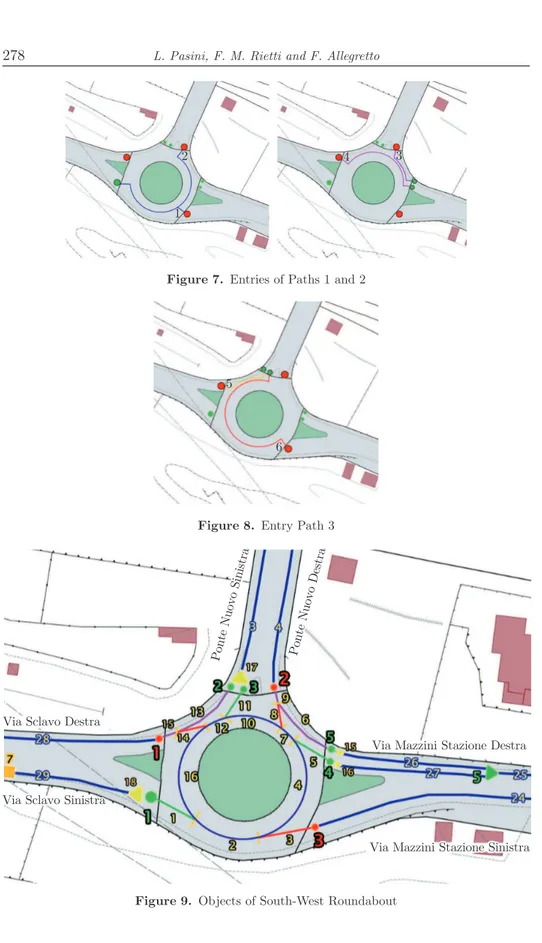
Figure 6. South-West Roundabout
The Figure 6 shows that entry-1 is composed of one lane, while the other two are both composed of two lanes. This means that, when the paths of each vehicle are analyzed, the road rules must be considered, since when there is a double entry, the right lane must be used exclusively to come out from the exit immediately following the entry. The travelling direction within the roundabout is composed of a single lane, but in the double entry case, an overlap of two vehicles within the path could be created. Lastly, all the exits are composed of one lane.
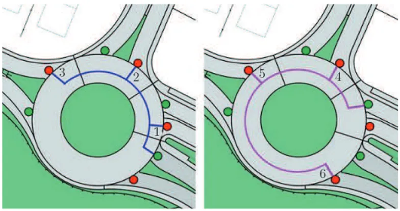
In the Figures 7, 8, all the paths in the South-West roundabout are shown. The Figure 9 shows instead all the objects of the South-West roundabout.
3.3. North-East Roundabout
Roundabout 3, located to the North-East of the analyzed system, allows the inflow and outflow of vehicles from two streets outside the system (Via Bracci and Via Grondaie) and from two streets inside the system (Ponte Malizia and
Figure 7. Entries of Paths 1 and 2
Figure 8. Entry Path 3
Via Lombardi). Coming out of roundabout 3, drivers will have two possibilities: (1) they will be able to reach the South-East roundabout, continuing on Ponte Malizia; (2) or they will be able to reach the North-West roundabout, continuing on Via Lombardi (Figure 10).
Figure 10. North-East Roundabout
The image above shows that roundabout 3 has four entries and 4 exits. It is only entry-2 that is composed of one lane, while the others are composed of two lanes. This means that, as has been already said about roundabout 2, when the paths of each vehicle are analyzed, the road rules must be considered since when there is a double entry, the right lane must be used exclusively to come out from the exit immediately following the entry. The travelling direction within the roundabout is composed of a single lane, but in the double entry case, an overlap of two vehicles within the path could be created. Lastly, all the exits are composed of one lane.
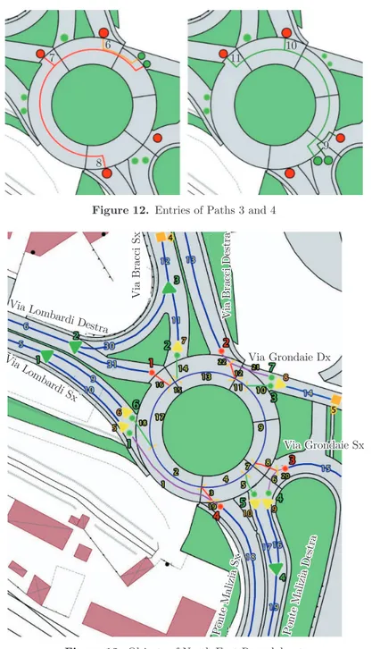
The Figures 11, 12 shows all the paths in the North-East roundabout. The Figure 13 shows instead, all the objects of the North-East roundabout.
Figure 12. Entries of Paths 3 and 4
Figure 13. Objects of North-East Roundabout
3.4. South-East Roundabout
Roundabout 4, located to the South-East of the analyzed system, allows the inflow and outflow of vehicles from two streets outside the system (Via Sardegna and Via Mazzini Centro) and from two streets inside the system (Ponte Malizia and Via Mazzini Stazione). Coming out of roundabout 4, drivers will have two
possibilities: (1) they will be able to reach the North-East roundabout, continuing on Ponte Malizia; (2) or they will be able to reach the South-West roundabout, continuing on Via Mazzini Stazione (Figure 14).
Figure 14. Objects of South-East Roundabout
The Figure 14 shows that the roundabout has four entries and four exits. The entries, as well as the exits, are composed of a single lane; even the inside lane of the roundabout is single.
In the Figures 15, 16, all the paths in the South-East roundabout are shown. The Figure 17 shows all the objects of the South-East roundabout.
Figure 15. Entries of Paths 1 and 2
4. Tracking procedure
In this section the necessary procedure to generate the main file that will be given as the input to the graphic engine for it to work is analyzed. At first, the files that are created during or at the end of the simulation run will be shown. These files are described in detail below:
Figure 16. Entries of Paths 3 and 4
Figure 17. Objects of South-East Roundabout
• RIS.txt: this file is created during the simulation. It makes a system snapshot every 5 seconds; it basically tracks all the objects inside the model (roads, multiplexers, crossroads, input and output sections). It allows an accurate system visualization at a particular chosen moment;
• FLUSSI.txt: this file is created at the end of the simulation. It allows comparing the number of vehicles that entered during the simulation and the vehicles that actually entered (based on the flows table for the City of Siena);
• INCROCI.txt: this file is created during the simulation. It collects all the data useful to verify each crossroad situation every 5 seconds (incoming queues, presence inside and outside the crossroad);
• TABELLA.txt: this file records summary data concerning the general sys-tem situation; more in detail, this information concerns incoming crossroads queues, presence inside them and along the roads;
• FLU INT.txt: this file collects data concerning the input stream of the system through the crossroad multiplexer. It allows verifying the difference between simulated data and real data;
• FLU INT.csv: this file, as the FLU INT.txt file, collects data concern-ing the input stream of the system through the crossroad multiplexer but it is saved in a different format file. This kind of a format file is useful to allow analysis of data in the graphic simulation;
• FLU OUT.txt: this file collects data concerning the output stream of the system through the crossroad multiplexer. It allows verifying the difference between simulated data and real data;
• FLU OUT.csv: this file, as the FLU OUT.txt file, collects data con-cerning the output stream of the system through the crossroad multiplexer but it is saved in a different format file. This kind of a format file is useful to allow analysis of data in the graphic simulation;
• CarSystem.csv: this file allows following the vehicle path from entering into the system, through several components (roads, roundabouts, input and output sections), until the exit. This file will be given as the input to the graphic engine for it to work correctly.
At the end of the simulation, the TS WRITE procedure reworks the queuing network model simulation data to the CarSystem.csv file, that is finalized to the graphic display. The procedure written in Qnap2 programming language [2] is given below.
/DECLARE/
PROCEDURE TS WRITE;
INTEGER I,J,IDX SWP,PROG FIN,PROG RAL; BOOLEAN SWAP; REAL TMP; BEGIN WRITELN(TrcVehic, "</VS>"); CLOSE(TrcVehic); TESTFLU; INT FLU; PROG FIN := 0; PROG RAL := 0;
FOR I:=1 STEP 1 UNTIL N CUR DO BEGIN IDX#(I) := I;
END; &FOR SWAP := TRUE;
WHILE (SWAP) DO BEGIN SWAP := FALSE;
FOR I:=1 STEP 1 UNTIL N CUR-1 DO BEGIN
IF(V TS#(IDX#(I)).TIME ENTRY > V TS#(IDX#(I+1)).TIME ENTRY) THEN BEGIN
IDX SWP := IDX#(I+1); IDX#(I+1) := IDX#(I); IDX#(I) := IDX SWP;
- V TS#(IDX#(I)).TIME ENTRY; SWAP := FALSE;
END;
IF(SWAP AND (J = N CUR)) THEN BEGIN
V TS#(IDX#(I)).PATH := V TS#(IDX#(I)).PATH // "-" // "OUT"; V TS#(IDX#(I)).TIME LIVE := 1;
END; END; END;
FOR I:=1 STEP 1 UNTIL N CUR DO BEGIN IF(V TS#(IDX#(I)).TIME LIVE > 0) THEN BEGIN;
PROG FIN := PROG FIN + 1;
TMP := V TS#(IDX#(I)).TIME LIVE-V TS#(IDX#(I)).SVC TIM IN; IF (TMP < 0) THEN TMP := 0.;
J:=1+CHRFIND(V TS#(IDX#(I)).PATH,"-");
IF (SUBSTR(V TS#(IDX#(I)).PATH,1,1) <> "S") THEN TMP := 0.; IF (SUBSTR(V TS#(IDX#(I)).PATH,J,J) <> "S") THEN TMP := 0.; WRITELN(FILE TS,PROG FIN,",",V TS#(IDX#(I)).TIME ENTRY:8:2,",",
V TS#(IDX#(I)).PATH,",",V TS#(IDX#(I)).TIME LIVE:8:2,",", V TS#(IDX#(I)).ID
&,",",TMP );
IF(TMP > 0.01) THEN BEGIN
PROG RAL := PROG RAL + 1;
WRITELN(FIL RALL,PROG RAL,",",V TS#(IDX#(I)).TIME ENTRY:8:2,",", V TS#(IDX#(I)).PATH,",",V TS#(IDX#(I)).ID,",",TMP:8:2); END; END; END; CLOSE(FILE TS); CLOSE(FIL RALL);
PRINT("N. Veichles Generated=",N VEC); END;
As shown previously, all the results obtained from the simulation are recorded inside a text file or a csv file, each of them with an appropriate structure according to the obtained useful information. The file that is going to be analyzed in detail is CarSystem.csv; it allows following the vehicle path from entering into the system, through several components (roads, roundabouts, sections), until the exit. Moreover, the CarSystem.csv file, will be given as the input to the graphic simulation and it will allow following the queuing model simulation outgoing data.
The need to develop a function to track trajectories of vehicles inside the system, depends on the necessity to develop a graphic simulator, so that it could verify the queuing network model simulator effectiveness and so as to evaluate what happens inside the system in an easier and clearer way. This procedure allows solving and verifying any possible queuing model simulation program code problem. The choice to record the data to a csv file format depends on the graphic engine needs of this kind of file to reuse easily internal data; vehicle data (creation and entrance into the system, road crossing, internal sections transit, etc.) These are registered sequentially while events are happening, determining alternation of information concerning different vehicles. The CarSystem.csv file is created at the end of the simulation, so that data can be sorted, becoming useful to the graphic simulator. In the picture below it is possible to see an extract from the CarSystem.csv file to understand how it is structured (Figure 18).
SpawnTime PathToFollow DisappearTime ID QNAP 1 1.94 29-S21 15.00 7 2 3.88 29-S21 15.00 8 3 5.71 12-11 3.00 4 4 5.82 29-S21 15.00 9 5 6.00 20-S419 15.00 2 6 7.69 14-S310 15.00 5 7 7.76 29-S21 15.00 11 8 8.71 11-S314 6.00 4 9 9.70 29-S21 15.00 14 10 10.00 8-S21 15.00 1 11 10.53 22-S423 15.00 3 12 11.42 12-11 3.00 10 13 11.64 29-S21 15.00 15 14 12.00 20-S419 15.00 12 15 13.04 1-S18 15.00 6 16 13.58 29-S21 15.00 19 17 14.42 11-S314 6.00 10 18 14.71 S314-S315 0.80 4 19 15.38 14-S321 15.00 13 20 15.51 S315-S317 0.60 4 21 15.52 29-S21 15.00 22 22 16.11 S317-S32 2.60 4 23 16.94 S21-S22 1.40 7 24 17.13 12-11 3.00 18 Figure 18. CarSystem.csv
second section will be the first one in the following path to follow; in that way, a chain that represents the entire vehicle path will be created. Paths generated by unifying all the system sections have been rebuilt precisely inside the graphic simulator;
• DisappearTime: this value is the amount of time required by the vehicle to tread the path to follow;
• ID QNAP: this value is the id that the QNAP simulator associates to each vehicle. It is useful during the graphic simulation in order to recognize the vehicles on the road.
5. Graphic Simulation
This section concerns the graphic simulation created with Unreal Engine 4. Firstly, it will be explained what Unreal Engine 4 is and why it has been used. Secondly it will be shown how the simulation model, composed of scenery and actors, was created. As far as the scenery is concerned, it will be shown how the road graphic model was rebuilt through AutoCAD 2D and Rhinoceros 3D. As far as the actors are concerned, it will be explained what their role in the scenery is. Lastly, it will be explained how UE4 is powered by the CarSystem file and how they work to achieve a correct simulation operation.
The Unreal Engine is a game engine developed by Epic Games, first showcased in 1998 in Unreal, a first-person shooter game. Although it was originally developed for first-person shooters, it has been successfully used in a variety of other genres, including stealth, MMORPGs, and other RPGs. Its code written in C++, the Unreal Engine features a high probability degree, and is a tool used by many game developers today. However, in recent versions, this tool is used to create 3d architectural renderings, and graphic simulations too. This is possible thanks to Blueprint Visual Scripting that allows anyone to easily interface with programming. The use of blueprints allows managing the author level, object and game-play behaviors, modify the user interface, adjust input controls and much more. Blueprint visual scripting comes with a built-in debugger that can be used to interactively visualize the graphic flow and inspect property values while testing simulation. It is also possible to freeze the simulation at any time, and to audit its state by setting breakpoints on individual nodes in Blueprint graphs.
Before proceeding with the UE4 steps used to let the simulator work, it will be explained how the simulation model has been realized. It is composed of two basic components:
• Scenario • Actors
5.1. Scenario
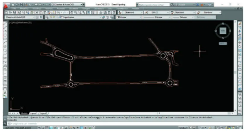
A scenario is a basic component of motor games. In our case, it was created using planimetry and level curves, taken from the Siena City website to reflect real road coordinates and ground morphology of the analyzed area. The second time, it was only the area of interest that was cut to make a 2D realistic model, using AutoCAD.
Figure 19. AutoCAD Model
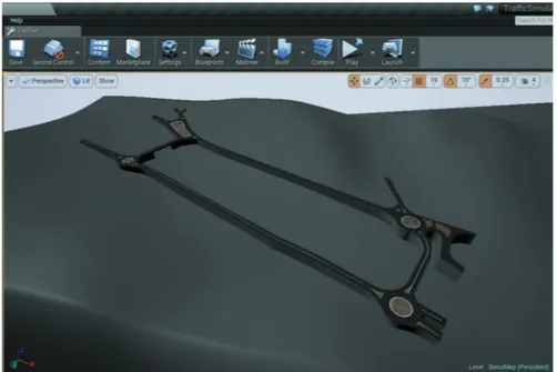
The 3D model was created importing the 2D model in Rhinoceros, com-mercial 3D computer graphics and computer-aided design (CAD) application soft-ware. In the Figure 20 it is possible to see the entire model in Rhinoceros.
Finally, the file is converted from 3D to FBX; the model is then imported in UE4, and the static scenery, on which the graphic simulation will be built, is obtained (Figure 21).
5.2. Actors
Actors are another essential component of motor games; in that case two kinds of actors were used for the graphic simulation:
• Sedan: the vehicle actor that appears in the road system (Figure 22); • Camera: the actor positioned on the 4 roundabouts; it shows what happens
during the simulation (Figure 23).
In the following text it will be explained in detail how these actors are powered by the CarSystem file, inside UE4.
Thanks to this file it is possible to create an actor with a specific To Do, and at an amount of time T , in a specific point (X,Y,Z) of the scenario. The
Figure 20. Rhinoceros Model
Figure 21. UE4 Model
CarSystem file is generated through the queuing network model simulator, and it allows the process just described to be used for to the correct graphic simulator work. Uploaded csv inside UE4 is shown in the Figure 24.
Vectors concerning the 4 table sections are then created through it (Fig-ure 25).
Figure 22. Vehicle Actor
Figure 23. Camera Actor
Figure 25. Array creation
In detail, the vectors created are the following:
• Path To Follow Vector: this vector contains 2 values, in a string format, collected during the simulation; the first one concerns the point where the vehicle appears, while the second one where it disappears. Moreover, the second one will be the first one of the following path, so that a chain, representing the entire vehicle path, will be created;
• Spawn Time Vector: this vector contains the time concerning the ap-pearance of a vehicle on a specific path to follow;
• Disappear Time Vector: this vector contains the time concerning the amount of time required to tread all the paths to follow;
• ID QNAP Vector: this vector contains the id associated to each vehicle by the QNAP simulator.
The Figure 26 shows how paths were created through the Path To Follow data. The first one represents roundabout 1, used as an example.
The picture on the left shows the North-West roundabout, with all the rebuilt paths; on the right side there are all the path names, which match the CarSystem.csv. ones. The Spline Array is created from these path names; it contains the name of each pair of points that will be researched inside the path to follow the vector. The graphic simulator paths and those of the queuing network model simulator are compared in the Figure 27.
Now we describe the actors mentioned previously, powered by the system, and how they are used. The sedan actor was built using UE4 default methods, linked to a generic vehicle object. When the simulation is launched, for each EventTick, the SpawnTime is checked to verify if a vehicle has to appear or not in a specified amount of time. If a match is found, through the SpawnActor method, (which takes PathToFollow in input, the DisappearTime and the IDQNAP of the examined vehicle), the vehicle appears on the road system, where it will follow the given path to a determined LifeTime (vehicle lifetime in a determined path).
Figure 26. Path creation in Unreal Engine 4
Figure 27. Path differences between Unreal Engine 4 and queuing network model
Once the LifeTime is reached, the vehicle disappears and then reappears in the adjacent path, until it disappears through a roundabout Output Section. That method concerns all the vehicles inside the CarSystem.csv file. The SpawnActor method in BluePrint is shown in Figure 28.
For the Camera Actor, 4 different kinds were made and placed on the 4 roundabouts. The Figure 29 shows the simulator screen for each roundabout; it allows a complete system view, so that it will be possible to examine the graphic simulation and to verify if it works correctly.
Figure 28. Spawn Actor Method
Figure 29. North-West Roundabout
Figure 31. North-East Roundabout
Figure 32. South-East Roundabout
6. Conclusions
In our previous works [1, 3–6], we illustrate how, basing on the above approach to specification, it becomes possible to construct a file describing a street system. Thus, given a street system, we will be able to associate a description file called Model.dat. Subsequently we have defined a procedure, called BuildMod, that will automatically generate a simulator of the traffic system in question. In fact, when executed, the BuildMod procedure reads the data from the Model.dat description file generating the queuing network model that simulates the traffic system.
In the present work we have illustrated how we adapted the old procedure to study a new urban system and, through a new tracking procedure, how we developed a graphic simulation able to reinterpret the data from the queuing network model simulation, in order to make it easier to check the effectiveness of the simulator and to have a graphical way to analyze the data.
In a future work, we will present how to combine textual research operation concerning traffic simulation into the virtual reality output. To reach this
achieve-• mark a road point as the input or output;
• mark a point as a multiplexer or road multiplexer; • mark a point as a semaphore.
This data can be used to write the first part of the Model.dat file, with an accuracy of one to one about the road lengths, the path to follow and the average road speed. The data can be stored in the Model.dat file or the output can be changed to a split data collection in multiple CSV files. To reach this achievement we should rewrite the input routine in the “costruzione.QNAP” file.
From classic input forms, the user will input: • the rules to generate the input flows of vehicles; • the rules to assign the path to follow;
• the rules for the roads capacity.
In this package scenario, the simulation can also be realized without real data, but only using opportune rules, and letting the graphic engine show the traffic performance over time.
References
[1] Pasini L and Sabatini S 2016 TASK Quart. 20 (1) 9 [2] Simulog QNAP2 V9 Reference Manual
[3] Pasini L and Feliziani S 2013 TASK Quart. 17 (3) 155 [4] Pasini L and Feliziani S 2010 TASK Quart. 14 (4) 405
[5] Pasini L, Feliziani S and Giorgi M 2005 TASK Quart. 9 (4) 397
[6] D’Ambrogio A, Iazeolla G, Pasini L and Pieroni A 2009 Simulation Modelling Practice