Algebraic geometry over a field of positive
characteristic
Luca Giuzzi
∗Lectures given by Prof. J.W.P. Hirschfeld
Abstract
Curves over finite fields not only are interesting structures in themselves, but they are also remarkable for their application to coding theory and to the study of the geometry of arcs in a finite plane. In this note, the basic properties of curves and the number of their points are recounted.
Keywords: Algebraic geometry, Finite fields MSC (2000): 51E22, 11G20, 94B05
Preface
These notes were inspired by the lectures given by Prof. J.W.P. Hirschfeld at the “Summer school Giuseppe Tallini on finite geometry” held in S.Felice del Benaco (Brescia) in July 1998. The following topics are discussed:
1. Fundamental definitions;
2. When is a projective algebraic set empty? 3. Plane curves;
4. The Riemann–Roch theorem; 5. Applications to coding theory;
6. The number of rational points and the Hasse–Weil theorem; 7. Equality in the Hasse–Weil bound;
8. The St¨ohr–Voloch theorem.
Acknowledgements: The author wishes to thank Prof. J.W.P. Hirschfeld for his constant advice
and support in the realisation of these notes.
1
Fundamental definitions
1.1
Algebraic definitions
Let R be a commutative ring.
(1) An ideal I ⊆ R is a subring of R such that, for any F ∈ R,
F I := {F G : F ∈ I} ⊆ I.
(2) An ideal I of R is principal if there exists an element F ∈ I such that
I = hF i = {F G : G ∈ R}.
(3) An ideal I is prime if F G ∈ I implies
F ∈ I or G ∈ I.
(4) An ideal I is maximal if there exist no ideal J of R such that J 6= R, J 6= I and
I ⊂ J.
(5) Any maximal ideal is prime.
(6) An ideal I is homogeneous if it is generated by homogeneous polynomials. (7) A ring R is an integral domain if, for any F, G ∈ R,
F G = 0 ⇒ F = 0 or G = 0.
(8) The residue class ring of R by a prime ideal is an integral domain. (9) The residue class ring of R by a maximal ideal is a field.
(10) A ring with only one maximal ideal is a local ring.
1.2
Geometric definitions
Some books on algebraic geometry and number theory that may be consulted are Fulton [2], Ireland and Rosen [7], Joly [8], Koblitz [9], Pretzel [12], Schmidt [13], Seidenberg [15], Stichtenoth [17], Thomas [19], van Lint and van der Geer [20], Walker [21].
Let K be an arbitrary field. For most purposes here, K is assumed to be either the finite field Fqof q elements or its algebraic closure Fq.
(1) An Affine n−space over K is
AG(n, K) = An(K) = {x = (x
(2) Given x∗ = (x0, x1, . . . , xn), y∗ = (y0, y1, . . . , yn) in An+1(K)\{(0, . . . , 0)}, let x∗ ∼ y∗if
there exists λ ∈ K\{0} with yi = λxifor all i; write the equivalence class of x∗ as P(x∗).
Then, the projective n−space over K is
P G(n, K) = Pn(K) = {P(x∗) : x∗ ∈ An+1(K)\{(0, . . . , 0)}}.
(3) Let Rn = K[X1, . . . , Xn] and Rn= K[X0, X1, . . . , Xn]. For F in Rn, define F∗ in Rnas
F∗(X0, X1, . . . , Xn) = (X0)deg FF (X1/X0, . . . , Xn/X0).
We call the mapping which associates F∗ to F homogenisation.
(4) A subset V of AG(n, K) is an (affine) algebraic set if there exists S ⊂ Rnsuch that
V = {x ∈ AG(n, K) : F (x) = 0 for all F in S}.
Similarly, a subset V of P G(n, K) is a (projective) algebraic set if there exists S ⊂ Rn,
with all elements homogeneous, such that
V = {P(x∗) ∈ P G(n, K) : F (x∗) = 0 for all F in S}.
(5) Given an affine algebraic set V in AG(n, K), the ideal of V is the set of polynomials
I(V) = {F ∈ Rn : F (x) = 0 for all x in V}.
An affine algebraic set V is irreducible if there do not exist proper algebraic sets V1, V2
with V = V1 ∪ V2. Equivalently, V is irreducible if and only if its ideal I(V) is prime.
The pair consisting of an irreducible algebraic set V in AG(n, K) and its ideal I(V) is an
affine variety. The ideal I(V) of a projective algebraic set V in P G(n, K), is the ideal of
Rn generated by all homogeneous polynomials F such that F (x∗) = 0 for all P(x∗) in
V. Irreducibility is defined as in the affine case, that is an algebraic set V in P G(n, K) is
irreducible if and only if V is a homogeneous prime ideal in Rn. Analogously to the affine
case, a projective variety consists of an irreducible algebraic set in P G(n, K) together with its (homogeneous) ideal.
(6) The coordinate ring of an affine variety V in AG(n, K) is the residue class ring
Γ(V) = Rn/I(V).
The homogeneous coordinate ring of a projective variety V in P G(n, K) is
Γh(V) = Rn/I(V).
(7) The function field K(V) of an affine variety V is the quotient field of its coordinate ring
Γ(V); that is,
K(V) = {f /g : f, g ∈ Γ(V) with g 6= 0}
= {F/G : F, G ∈ Rnwith G(x) 6= 0 for all x ∈ V}.
Note that F/G = F0/G0 in K(V) if and only if F G0 − F0G = 0 in Γ(V).
In the projective case, an element f in Γh(V) has degree d if d is the smallest degree for
which there exists a homogeneous polynomial F such that f = F + Γh(V). The function
field K(V) of a projective variety V is defined as
K(V) = {f /g : f, g ∈ Γh(V) of the same degree with g 6= 0}
= {F/G : F, G ∈ Rnof the same degree with G(x∗) 6= 0 for all P(x∗) ∈ V}.
Both in the affine and in the projective case, the dimension of V is the transcendence degree of K(V)/K. Hence, the dimension of V is r if r is the smallest integer such that K(V) is a finite algebraic extension of the field K(t1, . . . , tr), where t1, . . . , tr are independent
transcendental elements over K. If r = 1, then V is a curve.
The dimension of V may also be defined as the length minus one of the longest chain of irreducible algebraic varieties V0 ⊂ . . . ⊂ Vr = V contained in V. The two definitions are
equivalent.
(8) Given a point x of the affine variety V, the local ring at x is
Ox(V) = {f /g : f, g ∈ Γ(V) with g(x) 6= 0};
the unique maximal ideal of Ox(V) is
Mx(V) = {f /g : f, g ∈ Γ(V) with f (x) = 0, g(x) 6= 0}.
The local ring consists of all the elements of the function field of the variety which are defined at the point x; the maximal ideal at x provides a representation of the point x itself in the function field.
By natural embeddings,
K ⊂ Γ(V) ⊂ Ox(V) ⊂ K(V).
(9) For K = Fq, write AG(n, K) = AG(n, q) and P G(n, K) = P G(n, q). Given F1, . . . , Fr
in Rn, with x = (x1, . . . , xn) and x∗ = (x0, x1, . . . , xn) let
V(F1, . . . , Fr) = {x ∈ AG(n, q) : F1(x) = . . . = Fr(x) = 0}, V∗(F∗
1, . . . , Fr∗) = {P(x∗) ∈ P G(n, q) : F1∗(x∗) = . . . = Fr∗(x∗) = 0}.
2
When is a projective algebraic set empty?
Consider the following quadrics in P G(3, q):V1 = V(f (X0, X1) + λg(X2, X3)),
V2 = V(f (X0, X1) + µg(X2, X3)),
with λ 6= µ and f, g binary quadratic forms irreducible over Fq. Then, V1∩ V2 = ∅, since any
common points P(x0, x1, x2, x3) of the two quadrics must satisfy f (x0, x1) = g(x2, x3) = 0;
it makes no difference whether f and g are distinct or not. Note that the sum of the degrees of the quadrics is greater than the dimension of the space. The generalisation of this observation is the Chevalley–Warning theorem for affine algebraic sets [13, Chapter 4], which was given in its projective version by Segre [14].
The idea is that an algebraic set can be empty if and only if the degree of the polynomials which define it is high enough, when compared with the dimension of the ambient space.
Theorem 2.1. Let d1, . . . , dr be positive integers with d1+ . . . + dr = d.
(a) (i) There exist F1, . . . , Fr in Rn of degrees d1, . . . , dr with V(F1, . . . , Fr) = ∅ if and
only if d > n.
(ii) There exist F1, . . . , Fr in Rn of degrees d1, . . . , dr with V∗(F1∗, . . . , Fr∗) = ∅ if and
only if d > n.
(b) When d ≤ n, then, for any F1, . . . , Fr in Rn with N = |V(F1, . . . , Fr)| and N∗ =
|V∗(F∗
1, . . . , Fr∗)|,
(i) N ≥ qn−d;
(ii) N ≡ 0 (mod p); (Warning) (iii) N∗ ≥ 1 + q + q2+ . . . qn−d; (iv) N∗ ≡ 1 (mod p).
Let f : Fq → Fq be any function. Then, Lagrange’s Interpolation Formula expresses f as a
polynomial, which will be written using the same notation:
f (X) = X t∈Fq −f (t)X q− X X − t (2.1) = X t∈Fq f (t)[1 − (X − t)q−1]. (2.2)
To prove the theorem, this formula will have to be generalised. Consider F ∈ Rn:
F (X1, . . . , Xn) = X
ai1,...,inX1
i1. . . X
nin. (2.3)
In any finite field Fq, the relation
holds. There exists a unique ˆF ∈ Rnof degree q − 1 in each Xi equivalent to F : ˆ F (X1, . . . , Xn) = q−1 X i1=0 . . . q−1 X in=0 ˆai1,...,inX1 q−1−i1. . . X nq−1−in, (2.4) ˆ F (X1, . . . , Xn) ≡ F (X1, . . . , Xn) mod (X1q− X1, . . . , Xnq− Xn). (2.5)
Observe that the values of ˆF over Fq are exactly the same as the ones of F , even if the two
polynomials cannot be identified. In particular given any F , the forms of ˆF over Fqand Fqiare
different. So, for all (c1, . . . , cn) ∈ (Fq)n, ˆ F (c1, . . . , cn) = F (c1, . . . , cn). (2.6) Let χc1,...,cn(X1, . . . , Xn) = n Y i=1 [1 − (Xi− ci)q−1]; (2.7)
be the characteristic function of the set {c1, . . . , cn}; thus,
χc1,...,cn(x1, . . . , xn) =
½
1 if (x1, . . . , xn) = (c1, . . . , cn),
0 if (x1, . . . , xn) 6= (c1, . . . , cn). (2.8)
Hence, ˆF can be given explicitly as follows:
ˆ
F (X1, . . . , Xn) =
X AG(n,q)
F (c1, . . . , cn)χc1,...,cn(X1, . . . , Xn); (2.9)
this provides the “generalised Lagrange’s Interpolation Formula”.
Comparing the coefficients of X1q−1. . . Xnq−1on both sides of (2.9) shows that
ˆa0,...,0 = (−1)n
X AG(n,q)
F (c1, . . . , cn). (2.10)
Lemma 2.2. Let d be an integer with 0 ≤ d ≤ q − 1. Then,
X t∈Fq td = ½ 0 if d 6= q − 1, −1 if d = q − 1. Proof: If d = 0, X x∈Fq xd= X x∈Fq 1 = q = 0.
When 0 < d < q − 1, let us take z to be a generator of the cyclic group F∗q; then, zd 6= 1. On the other hand, as x runs over Fq, also zx runs over all the elements of Fq; thus,
X x∈Fq xu = X x∈Fq (zx)u = zu X x∈Fq xu
is possible if and only if the sum is zero. If d = q − 1, X x∈Fq xd = 0 + X x∈F? q xq−1 = X x∈F? q 1 = q − 1 = −1. ¤
Lemma 2.3. Let F in Rnhave degree d < n(q − 1). Then, X
x∈AG(n,q)
F (x) = 0.
Proof: By linearity, it suffices to consider the case in which F is a monomial. If F (x) =
Xd1 1 X2d2. . . Xndn, then X x∈AG(n,q) F (x) = n Y i=1 X xi∈Fq xui i .
Since d1 + . . . + dn < n(q − 1), there is a dj with ndj ≤ d ≤ n(q − 1). So, by the previous
lemma, X
xj∈Fq xdj
j = 0,
and the result follows. ¤
Proof of parts (ii) and (iv) of Theorem 2.1
With X = (X1, . . . , Xn), let G(X) = r Y i=1 £ 1 − Fi(X)q−1 ¤ .
Then, G has degree d(q − 1) < n(q − 1). So, by Lemma 2.3, Px∈AG(n,q)G(x) = 0. On the other hand, Fi(x)q−1 = 1 for any x ∈ AG(n, q), unless Fi(x) = 0. Hence, G(x) = 0 unless x
is a common zero of F1, . . . , Fr, in which case G(x) = 1. Therefore,
0 = X
x∈AG(n,q)
G(x) = N,
whence N ≡ 0 (mod p).
The projective version follows now readily. Let N0 = |V(F1∗, . . . , Fr∗)|; that is, N0 counts the number of zeros in AG(n + 1, q) of V(F1∗, . . . , Fr∗). Then, N∗ = (N0 − 1)/(q − 1). As
N0 ≡ 0 (mod p), so N∗ ≡ 1 (mod p). ¤
For a proof of the following improvement to the theorem, especially relevant when d is small compared to n, see [1, 8].
Theorem 2.4. With the hypotheses of Theorem 2.1, let d < n and let e be an integer with
3
Plane curves
Our attention will be mostly restricted to plane curves. First, some precise definitions are re-quired. Let F in Fq[X, Y, Z] be homogeneous. As in §1, let
V(F ) = {P(x, y, z) ∈ P G(2, q) : F (x, y, z) = 0}.
Then, the curve defined by F is
V = (q, V(F ), (F )) = V(F );
sometimes this curve may simply be referred to as F . The elements of V(F ) are the rational
points of V and (F ) is the ideal generated by F in Fq[X, Y, Z]. The polynomial F defines
a curve; however, in order to understand the geometry of this curve, the knowledge of zeros of F over Fq and over any extension of Fq is required: in fact, the zeros over Fq are not
always sufficient to recover F . Let Fq be the algebraic closure of Fqand write as P G(2, qi) the
projective plane over Fqi. An Fqi-rational point of V is a point P(x, y, z) in P G(2, qi) such
that F (x, y, z) = 0. Thus, an Fq-rational point of V is a rational point of V. A point of V is
simply an Fqi-rational point for some positive integer i. Also, let
V(F ) = {P(x, y, z) ∈ P G(2, Fq) : F (x, y, z) = 0}.
Hence, a point of V is just a point which is rational over the algebraic closure of Fq, that is a
point of V(F ).
A point of degree i of V is a point that is Fqi-rational but not Fqj-rational for j < i. A closed
point of degree i of V is a set {P, Pq, . . . , Pqi−1}, where P is a point of degree i.
A divisor D on V is an element of the free group generated by the closed points of V; in other words, D is a formal sum:
D = X
P ∈V(F )
nPP,
where nP ∈ Z and nP = 0 for all but a finite number of P . We say that D = P
nPP is an Fq-divisor if, when P ∈ Supp(D) and P is of degree i, then P0 ∈ Supp(D) and nP0 = nP, for
all P0 in the closed point {P, Pq, . . . , Pqi−1}. The Fq-divisors form the subgroup DivFq(V) of
Div(V).
The support of D is
Supp(D) = {P : nP 6= 0}.
The degree of D is deg D =PnP. The divisors on V form a free Abelian group Div(V).
A divisor D is effective if nP ≥ 0 for all P ∈ Supp(D). This allows the introduction of a
partial order on the divisor group: we say that
D ≥ D0
if and only if D − D0is effective.
A singular point of V is a point P = P(x, y, z) such that every line through it intersects V twice in P. That implies that P(x, y, z) has to satisfy
∂F ∂X = ∂F ∂Y = ∂F ∂Z = 0 at (x, y, z).
Note that a singular point does not have to be in V(F ), but may be in V(F ). For example, consider q to be odd and let ν2 = −1. Then, with
F = (X2+ Y2)2+ (X2− Y2)Z2+ Z4,
the curve V has the two singular points P(ν, 1, 0) and P(−ν, 1, 0), which are rational when
q ≡ 1(mod4) but not when q ≡ −1(mod4).
Let now F be absolutely irreducible. Also, take U2 = P(0, 0, 1) and write
F (X, Y, 1) = Fs+ Fs+1+ . . . + Fm,
where Fs 6= 0 and each Fi is homogeneous in X and Y of degree i. Then, U2 has multiplicity
s on V; it is singular if s > 1 and an ordinary singular point if Fshas no repeated factors. The
factors of Fsare the tangents to V at U2. To find the properties of any other singular point, it is
possible to transform it to U2by a translation. The multiplicity of P on V is denoted by mP(V).
A line through P is said to be a tangent to V if it meets the curve with multiplicity k >
mP(V).
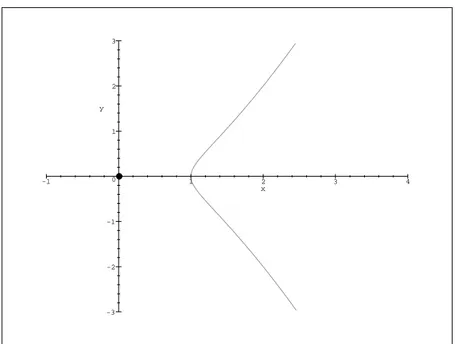
We say that a double point P is a node if there are exactly two tangents passing through it; for example, consider the origin for the curve
F = Y2− X2− X3
defined over the reals.
A cusp is a double point at which there is only one tangent; the origin for
F = Y2− X3
provides an example.
An isolated double point is a double point at which the tangents lie in a quadratic extension of the field, and thus are not visible. As an example we can consider the real curve
F = Y2+ X2− X3.
Clearly, there are no isolated double points over algebraically closed fields.
In fact, there are two numbers that need to be distinguished for a (plane) curve V. Let N1∗ be the number of rational points on a non-singular model, and let R = |V(F )|. In the case that
q = 2 and
F = (X2+ XY + Y2)Z + X3,
R = 4, N∗
1 = 3. Here, V(F ) = {P(0, 0, 1), P(1, 1, 1), P(1, 0, 1), P(0, 1, 0)}, but P(0, 0, 1) is
an isolated double point; that is, the tangents in it lie over F4; thus, the point is not visible on a
-1 -0.5 0 0.5 1 -1 -0.5 0.5 1 x Figure 1: Node
The number N1∗ is generalised to Ni∗, which is the number of Fqi-rational points on a
non-singular model of V.
The same definitions applies also to affine curves.
As an example, consider the affine Fermat cubic given by
f = X3+ Y3+ 1 :
(a) over F2 there are two rational points (0, 1) and (1, 0); hence, N1 = 2;
(b) over F4 := {0, 1, ω, ω2} there are six rational points:
(0, 1), (0, ω), (0, ω2), (1, 0), (ω, 0), (ω2, 0),
whence N2 = 6.
Passing to the projective case, we consider f∗ = X3+ Y3+ Z3and we get (a) N1∗ = 3;
(b) N2∗ = 9.
Once the multiplicity of a point on a curve has been defined, it is possible to introduce the intersection multiplicity of two curves at a point. Here, such number is not shown to exist; however, effective rules for calculating it are given.
Let V = V(F ) and W = V(G). Then, the intersection multiplicity of V and W at P , denoted by I(P, V ∩ W), has the following properties.
-1 -0.5 0 0.5 1 0.2 0.4 0.6 0.8 1 x Figure 2: Cusp I. I(P, V ∩ W) = I(P, W ∩ V).
II. (a) I(P, V ∩ W) = 0 if P 6∈ V(F ) ∩ V(G);
(b) I(P, V ∩ W) = ∞ if V and W have a common component through P ; (c) I(P, V ∩ W) ∈ N otherwise.
III. If τ ∈ P GL(3, q) with Vτ = V0, Wτ = W0, P τ = P0, then I(P, V ∩ W) = I(P0, V0∩
W0).
IV. I(P, V ∩ W) ≥ mP(V)mP(W), with equality if and only if V and W have no common
tangent at P . V. If F = QFri
i , G = Q
Gsj
j , with Fi, Gj forms in Fq[X, Y, Z] and Vi = V(Fi), Wj = V(Gj), then
I(P, V ∩ W) =X
i,j
risjI(P, Vi∩ Wj).
VI. I(P, V ∩ W) = I(P, V ∩ H), where H = V(H), with H = G + EF and E is a form in
Fq[X, Y, Z] such that deg E = deg G − deg F ≥ 0.
VII. (B´ezout’s theorem) Over an algebraically closed field, if V of degree m and W of degree
n have no common component, then
X P
-3 -2 -1 0 1 2 3 y -1 1 2 3 4 x
Figure 3: Isolated double point The intersection divisor of V and W is the formal sum
V.W =X
P
I(P, V ∩ W)P ;
then, we can write Property VII as
deg(V.W) = mn.
In order to calculate I(P, V ∩ W), property III is used with P0 = U2, and then V and VI are
applied till IV can provide a final answer. As an example consider
F = Y Z − X2 G = Y Z2− X3.
By VI, the intersection multiplicity of F and G at any point is the same as that of G − XF =
Y Z2− XY Z = Y Z(Z − X) and F . There are no common components through F and G. By
V, we can consider the intersections of F with the three components of G, thus
F.Y = 2(0, 0, 1), F.Z = 2(0, 1, 0), F.(Z − X) = (0, 1, 0) + (1, 1, 1),
whence
F.G = 2(0, 0, 1) + 3(0, 1, 0) + (1, 1, 1)
-2 -1 0 1 2 -2 -1 1 2 x Figure 4: F and G
3.1
Mappings
A regular (or polynomial) map between two curves F and G is a function f : F → G defined by two elements f1, f2 of the coordinate ring of F such that
(x, y) ∈ V(F ) → (f1(x, y), f2(x, y)) ∈ V(G).
We say that φ ∈ K(F ) is defined at a point (x, y) ∈ F if there exist f, g ∈ Γ(F ) with
g(x, y) 6= 0 and
φ(x, y) = f (x, y) g(x, y).
A rational map φ : F → G is a pair φ1, φ2 ∈ K(F ) such that, if φ1, φ2 are defined at
(x, y) ∈ V(F ), then (φ1(x, y), φ2(x, y)) ∈ V(G).
An isomorphism is a regular map with an inverse regular map.
A birational isomorphism is a rational map with an inverse rational map.
The following results show the relationship between algebraic and geometric structures.
Theorem 3.1. The curve F is isomorphic to G if and only if
Γ(F ) ' Γ(G).
Theorem 3.2. The curve F is birationally isomorphic to G if and only if
Example 3.3. Let F = X, G = Y − X3and define f (0, t) = (t, t3). Then,
Γ(F ) = K[X, Y ]/(X) ' K[Y ]
and
Γ(G) = K[X, Y ]/(Y − X3) ' K[X].
The inverse of f is f−1(x, y) = (0, x) — clearly this is regular, as well as f is. It follows that
Γ(F ) ' Γ(G)
and the two curves are isomorphic.
Consider now F = X and G = Y2− X3and let f (0, t) = (t2, t3). The function f is clearly regular, but the inverse f−1(x, y) = (0, y/x) is not at the point (0, 0).
On the other hand, Γ(F ) = K[Y ] and Γ(G) = K[X, Y ]/(Y2− X3), whence
K(F ) ' K(Y ).
We can also verify that
K(G) ' K(Y /X) ' K(Y ) ' K(F ),
whence we obtain that F and G are birationally isomorphic even if not isomorphic.
The Zarisky topology in P G(2, K) is defined as the topology whose closed sets are inter-section of curves. Using this definition it is possible state the following result.
Theorem 3.4. If φ : P G(2, K) → P G(2, K) is an isomorphism on an open set, then φ it is a birational isomorphism of P G(2, K).
A point P of V(F ) with multiplicity m is an ordinary singular point if m ≥ 2 and the tangents at P are all distinct.
For example the singular point (0, 0) is ordinary for F = Y2−X2−X3in odd characteristic, but it is not ordinary for the curve F = Y2− X3.
Nodes are ordinary singular points, cusps are not.
Theorem 3.5. Let V be a curve in P G(2, K). Then, there exists a birational isomorphism φ of
P G(2, K) such that φ(V) has only ordinary singular points.
In fact, there exists an algorithm for constructing this birational map: it is based on the use of projectivities and of the standard quadratic transformation
(x, y, z) → (yz, zx, xy).
Let V be a curve with ordinary singular points P1, . . . , Pt of multiplicities s1, . . . , st. The
genus of V is the number
g = g(V) = 1
2(m − 1)(m − 2) −
Pt
i=112si(si− 1).
A curve V can be transformed into a curve X , not necessarily plane, with no singular points at all. Such a curve X is a non-singular model of V; any two such models are birationally isomorphic.
Example 3.6. Let V = {P(1, t, t2, t3) ∈ P G(3, K) : t ∈ K} ∪ {P(0, 0, 0, 1)} be the twisted cubic. Then there are three types of chords:
(1) tangent; (2) bisecant;
(3) 0-secant (that is, a bisecant with two non-rational contact points).
Through every point P ∈ P G(3, K) \ V there is exactly one chord. We say that the point P is of type i if there is a chord of type i through it. Then, the projection of V through P is a plane cubic with:
(a) a cusp if P is of type (1); (b) a node if P is of type (2);
(c) an isolated double point if P is of type (3).
Let V = V(F ) be a curve in P G(2, K). The points of a non–singular model X of V are the
places of V. We say that a place Q is centred at P if φ(Q) = P , where φ : X → V.
Any function φ ∈ K(X ) can be expanded at a simple point P as a formal power series
φ(t) =
∞ X
i=r
aiti.
The integer r is called the order of φ at P and it is denoted by the symbol ordP(φ). A formal
approach to this can be found in [15], pag. 82.
It is always possible to associate a divisor to φ. Roughly speaking, if φ = f /g then div(φ) = (φ) = X .f − X .g =
X
vP(φ)P,
and the valuation vP(φ) coincides with ordP(φ) as defined above. This divisor may be written
as the difference of two effective divisors: (φ)0− (φ)∞. In this expression, (φ)0is called divisor
of zeros and (φ)∞is the divisor of poles of φ. A divisor D such that there exists φ ∈ K(X ) with
D = (φ) is principal. All principal divisors have degree 0, but the converse is not true. The
quotient group between the group of all the divisors of degree 0 and the group of all principal divisors is denoted by the symbol C(X ). This group plays an important role in the study of the arithmetic and geometric properties of the curve X . In fact, over an algebraically closed field, C(X ) is usually denoted by Jac(X ) and has the structure of an algebraic variety with an Abelian group law. This variety is called the Jacobian variety of X .
Given a curve, we may ask ourselves how many effective Fq-divisors of a prescribed degree
i there are. Let Mi be this number.
As an example, consider again the Fermat cubic over F2. This curve has only P0 = (0, 1, 1),
P1 = (1, 0, 1) and P2 = (1, 1, 0) as F2-rational points; let also:
Q1 = (1, 0, ω), Q21 = (1, 0, ω2),
Q2 = (1, ω, 0), Q22 = (1, ω2, 0),
where F4 = {0, 1, ω, ω2}. Then, we have the following:
- Degree 1: P0, P1, P2, hence M1 = 3;
- Degree 2: 2P0, P0+ P1, etc. and Q0+ Q20, Q1+ Q21, etc. for a total of M2 = 9;
- Degree 3: With similar arguments we get M3 = 21;
- Degree r: we can prove Mr = 3(2r− 1).
In order to carry out our project more algebraic tools are needed; in fact, the geometry of curves is governed by the properties of local rings.
Theorem 3.7. Let R be a local ring that is not a field. Then, the following are equivalent:
(i) the unique maximal ideal M in R is principal;
(ii) there exists t ∈ R such that if z ∈ R\{0} then z = utn for a unique unit u and unique non-negative integer n.
Such a ring R is a discrete valuation ring (DVR); the element t is a uniformising parameter. Suppose, in this situation, that K is a subring of R isomorphic to R/M .
Theorem 3.8.
(i) For any z ∈ R, there is a unique λ in K such that z − λ ∈ M .
(ii) For any n ≥ 0, there are unique λ0, λ1, . . . , λnin K and zn ∈ R such that
z = λ0 + λ1t + . . . + λntn+ zntn+1.
Theorem 3.9.
(i) The point P on a curve V is simple if and only if OP(V) is a DVR.
(ii) In this case, the image L in Γ(V) of a line L = aX + bY + c that is not a tangent to V at
P is a uniformising parameter for OP(V).
The set of all places P of a curve V corresponds bijectively to the set of all the maximal ideals MP of the DVR’s of the curve.
In this more abstract setting, the valuation vP(φ) of a function φ ∈ OP(V) at a place
corre-sponding to the ideal MP can be defined to be the integer n such that φ = uLn where u is an
unit in OP(V).
In order to find n = vP(φ) for P in (φ)0, we write
to determine n = vP(φ) for P in (φ)∞, we write 1
φ = uL
n.
Example 3.10. Let us consider the Fermat cubic over the field F2 and label the set of its F4
-rational points as follows:
0 0 0 1 1 1 1 1 1
1 1 1 0 0 0 1 ω ω2
1 ω ω2 1 ω ω2 0 0 0
P0 P1 P2 P3 P4 P5 P6 P7 P8
.
Let φ1 = Y +ZX and φ2 = Y +ZY . Then,
div(φ1) = P1+ P2− 2P0,
div(φ2) = P3+ P4+ P5− 3P0.
This shows a remarkable property of divisors of functions; in fact, (1) deg div(φ) = 0;
(2) there is an equivalence relation on DivFq(X ) that is given by D0 ≡ D ⇐⇒ D0 = D + div(φ)
for some φ ∈ Fq(X ).
Example 3.11.
(Y + Z).F ≡ Y.F ≡ X.F
3P0 ≡ P3+ P4+ P5 ≡ P0+ P1+ P2
Theorem 3.12. Let P be a point on the irreducible curve V with local ring OP and maximal
ideal MP. Then, the multiplicity mP of P on V is
mP = dimK ¡
MPn/MPn+1 ¢
4
The Riemann–Roch theorem
The aim of this theorem is to count the number of rational functions with poles in a given divisor
D =PnPP . For any divisor D, define L(D) as
L(D) = {φ ∈ K(X ) : vP(φ) ≥ −nP};
that is, φ ∈ L(D) if and only if div(φ) + D is effective. Clearly, L(D) is a vector space over the field K. We want to compute its dimension l(D) := dim L(D). This is the same as asking for the maximal number of linearly independent curves cutting out divisors equivalent to D.
Theorem 4.1 (Riemann).
(i) Given an irreducible curve X , there exists a constant g ≥ 0 such that, for any divisor D,
l(D) ≥ deg D + 1 − g.
The smallest such g is the genus of X .
(ii) There exists an integer N such that, when deg D > N ,
l(D) = deg D + 1 − g.
(iii) The genus g is a birational invariant.
The Riemann–Roch theorem extends part (i) of Theorem 4.1 by giving explicitly the differ-ence between the two sides of the inequality. See [11], chapter 2 for the details.
Example 4.2. Consider as usual the Fermat cubic F over F4and let D = 3P0. Then, φ1, φ2 ∈
L(D) and g = 1; it follows that l(D) = l(3P0) = 3 + 1 − 1 = 3, whence
L(3P0) = h1, φ1, φ2i.
Let D be a divisor and let f0, . . . , fr ∈ L(D) be linearly independent. Then the set of
effective divisors
Dλ = div( X
λifi) + D
as λ0, . . . , λrvary in Fqis a linear series gnrof degree n and dimension r. The series is complete
if L(D) = hf0, . . . , fri; this is equivalent to say that there is no gsnwith s > r and grn⊂ gns.
A parameter space for grnis a P G(r, q) given by the bijection
Dλ → (λ0, . . . , λr).
Another way of viewing this is to define
f0 = 1, fi =
Fi
F0
for suitable polynomials F0, . . . , Fr. Then,
Dλ = X .(λ0F0+ . . . + λrFr);
that is, the series is cut out by the family of curves λ0F0+ . . . + λrFr.
In Example 4.2, the lines of the plane are a linear combination of Y + Z, X and Y and cut out a complete linear series g32on F .
For a gnr, we have l(D) − 1 = r, whence we can restate part (ii) of the theorem as follows: given a complete linear series gnr with n > N ,
r = n − g.
5
Applications to coding theory
It is possible to introduce the following distance function on any vector space V : for all x, y in
V , let
d(x, y) := |{i : xi 6= yi}|.
This distance is called the Hamming distance on V .
An [n, k, d]q-linear code C is a k-dimensional linear subspace of (Fq)n such that for all
x, y ∈ C with x 6= y we have
d(x, y) ≥ d.
The parameters are as follows:
n is the length of C; k is the dimension of C;
d is the minimum distance of C.
The elements of C are called words. The weight of a word is defined to be the number
w(x) = d(x, 0) = |{i : xi 6= 0}|.
For a linear code, the minimum distance is
d(C) = min
x,y∈Cx6=yd(x, y) = minx∈Cx6=0w(x).
Clearly, not all the parameters are independent.
Theorem 5.1 (Singleton). For a linear [n, k, d]qcode,
We say that a code is e-error correcting if the minimum distance d between its words satis-fies
d ≥ 2e + 1.
A code is an MDS code (Maximum Distance Separable code) if the Singleton bound is attained, that is, d = n − k + 1.
Usually a code is good if n is small and both k and d are fairly large. A generator matrix for C is a k × n matrix whose rows form a basis for C.
Example 5.2. Let
Pk := {f ∈ Fq[T ] : deg f < k} =< 1, T, . . . , Tk−1 >; Fq= {t1, . . . , tq};
C = {(f (t1), . . . , f (tq)) : f ∈ Pk}
Then, n = q and dim C = k. Since there are at most k − 1 zeros in any word, there are at least
q − (k − 1) non–zeros, hence
d = q − k + 1 = n − k + 1
and the code is MDS. The generator matrix G may be written as
G = 1 1 1 . . . 1 t1 t2 t3 . . . tq t2 1 t22 . . . t2q .. . tk−1 1 . . . tk−1q .
5.1
Construction of an algebraic geometry code
These codes were found by Goppa in 1981. Let (1) X be an algebraic curve over Fqof genus g;
(2) D = P1+ . . . + Pnbe a divisor, where all the Piare rational and distinct;
(3) E = m1Q1+. . .+mrQrbe a Fq-divisor where Qj 6= Pifor all i, j; thus, deg E = P mj = m; (4) θ be the map θ : ½ L(E) → (Fq)n f → (f (P1), . . . , f (Pn)) (5) C = C(D, E) := imθ = {(f (P1), . . . , f (Pn)) : f ∈ L(E)}.
Then, C is an [n, k, d]q-code whose parameters satisfy the following conditions. Theorem 5.3. If n > m > 2g − 2, then (i) k = m − g + 1; (ii) d ≥ n − m. Corollary 5.4. n − k + 1 − g ≤ d ≤ n − k + 1 Proof:
(i) This is the statement of Riemann’s theorem.
(ii) If f ∈ L(E) and w(θ(f )) = d, then f is zero at n − d points Pi1, . . . , Pin−d forming a
divisor D0 where deg D0 = n − d and D0 < D. Now divf + E is effective and no Pij
occurs in E; hence,
divf + E > D0. If we take the degrees of both sides, we obtain now
m > n − d,
as required.
By adding (i) and (ii) we get
k + d ≥ n − g + 1,
whence the corollary follows. ¤
Example 5.5. Let F = X3+ Y3 + Z3 be the Fermat cubic over F4, and, with the notation of
before, E = 3P0and D = P1 + . . . + P8. Then, we take as generator matrix
1 1 1 1 1 1 1 1 1 X Y +Z 0 0 1 ω2 ω 1 ω2 ω Y Y +Z ω ω2 0 0 0 1 1 1 = G.
Hence, n = 8, k = 3, 5 ≤ d ≤ 6. Since row 3 of G is a word of weight 5, it follows that
C(D, E) is an [8, 3, 5]4code with e = 2.
The relevance of algebraic geometry codes is that it is possible to determine good upper and lower bounds on their minimum distance.
6
Number of rational points and Hasse–Weil theorem
Assume C to be a plane curve of genus g defined over Fq, and let X be its non-singular model.
Also, let
(1) Nibe the number of points of V that are rational over Fqi;
(2) Msbe the number of effective Fq-divisors on V of degree s;
(3) Bj be the number of closed points of degree j.
We define the zeta function of X as
ζX(T ) = X DivFq(X ) Tdeg D = 1 + ∞ X s=1 MsTs. Lemma 6.1. (i) Ni = P j|ijBj. (ii) ζX(T ) = Q∞ j=1(1 − Tj)−Bj = exp( P∞ i=1NiTi/i).
Thus, the zeta function encodes information on the number of rational points of C over any extension of Fq.
Theorem 6.2. (Hasse–Weil)
ζX(T ) = f (T )/{(1 − T )(1 − qT )},
where
(i) f (T ) = (1 − α1T ) . . . (1 − α2gT ) ∈ Z[T ];
(ii) α1, . . . , α2g are complex numbers;
(iii) αjαg+j = q, j = 1, . . . , g; (iv) |αj| =√q, j = 1, . . . , 2g. Corollary 6.3. (i) Ni = 1 + qi− (αi1+ . . . + αi2g); (ii) |Ni− (1 + qi)| ≤ 2g p qi. Proof:
(ii) From (i), |Ni− (1 + qi)| = |αi1+ . . . + αi2g| ≤ |αi 1| + . . . + |αi2g| = 2gpqi. ¤
Example 6.4. Recall that
log f (T ) (1 − T )(1 − qT ) = (c1T + c2T 2+ . . .) −(c1T + c2T2+ . . .)/2 + . . . +(T + T2/2 + . . . +(qT + q2T2/2 + . . . = (1 + q + c1)T + (1 + q2+ 2c2− c21)T2/2 + . . . Hence, N1 = 1 + q + c1, N2 = 1 + q2+ 2c2− c21.
We now consider some special cases:
(1) If g = 0, then X is either a line or a conic.
ζX(T ) =
1
(1 − T )(1 − qT ).
We get c1 = 0, and Ni = 1 + qi for all i.
(2) F = X3+ Y3+ Z3 over F2; then,
ζF(T ) =
1 + c1T + 2T2
(1 − T )(1 − 2T ).
Since N1 = 3 = 1 + 2 + c1, we get c1 = 0; hence,
log ζF(T ) = X
(−1)(j−1)(2T2)j/j +XTi/i +X(2T )i/i.
This implies that
Nh = 1 + 2h for h odd 1 + 2h+ 21+h/2 for h ≡ 2(mod4) 1 + 2h− 21+h/2 for h ≡ 0(mod4) Corollary 6.5. (i) |N1− (1 + q)| ≤ 2g√q; (ii) N1 = 1 + q − (α1+ . . . + α2g); (iii) N2 = 1 + q2− (α21+ . . . + α22g).
Corollary 6.6. For a plane non-singular curve of degree d,
|N1− (1 + q)| ≤ (d − 1)(d − 2)
√ q.
7
Equality in the Hasse–Weil bound
The Hermitian curve U2,qis defined byF = X√q+1+ Y√q+1+ Z√q+1,
where q is a square. This gives an example of a curve V in which the upper bound in Corollary 6.5(i) is achieved. Here, g = 12(q −√q), whence
q + 1 + 2g√q = q + 1 + (q −√q)√q = q√q + 1 = N1.
Conversely, the curve U0 = (q2, V(F ), (F )), obtained taking the same equation F over GF (q2) archives the lower bound on the number of its rational points.
A curve V is maximal if N1 = q + 1 + 2g√q. Thus, U2,q is one example.
Theorem 7.1. Let V be a maximal curve. Then, the inverse roots satisfy
αi = −
√ q
for all i.
Proof: The result follows from Theorem 6.2 (iii) and Corollary 6.5 (ii). ¤
It can also be seen that the zeta function of a maximal curve V is
ζV(T ) =
(1 +√qT )2g
(1 − T )(1 − qT );
that of the Hermitian curve is
ζU2(T ) =
(1 +√qT )q−√q (1 − T )(1 − qT ).
In fact, the Hasse–Weil theorem provides a good bound when q is large compared to the genus g, but it is not so good when g is large compared to q.
Write Nq(g) := max N1, where N1is computed for non–singular curves of genus g over Fq
and define Aq := lim X g→∞ Nq(g) g .
From the Hasse–Weil theorem it follows that Aq≤ b2√qc. However, this can be improved.
Theorem 7.2 (Drinfeld-Vlˇadut¸). The parameter Aqsatisfies
Aq ≤
√ q − 1
8
The St¨ohr–Voloch theorem
In this section we summarise some background material concerning Weierstrass points and Frobenius orders from St¨ohr and Voloch [18].
Let us start by considering what happens in the case of the lines. The order sequence of a non-singular curve F with respect to the lines at a point P is given by the three numbers
min I(P, li ∩ F ),
i = 1, 2, 3, where
(1) l1is an arbitrary line of P G(2, q);
(2) l2contains P ;
(3) l3is the tangent TP.
For example, for the Hermitian curve U2,qthe order sequence is
(i) (0, 1,√q) if P is not rational; (ii) (0, 1,√q + 1) if P is rational.
In order to count the number of points of a plane curve F , we can consider a family of curves in the plane meeting F and apply some technique in order to count the intersections of members of this family with the given curve.
For a general curve F , a point of inflexion is a simple point P of F such that if TP is the
tangent at P to F , then I(P, TP ∩ F ) ≥ 3.
The Hasse–Weil theorem keeps track only of the singularities of F that turn up in the compu-tation of the genus; the St¨ohr-Voloch theory considers inflexions with respect to a given family of curves.
The essential idea is as follows: consider the action induced by the morphism
φ : (x, y, z) → (xq, yq, zq)
over Fqand let G(X, Y ) = F (X, Y, 1). The curve F is fixed by φ, and so are all its Fq-rational
points. Thus, we have that the set of all the Fq-rational points of F is contained in
{P ∈ V(F ) : φ(P ) = P }.
Write GX := ∂X∂G and GY := ∂G∂Y; then, the tangent at a point P = (x0, y0) of F can be written
as
Tp = GX(x0, y0)(X − x0) + GY(x0, y0)(Y − y0).
The following inclusion holds:
Now let H = (Xq− X)GX + (Yq− Y )GY, in order to be able to write
φ(P ) ∈ TP ⇐⇒ H(x0, y0) = 0,
and consider how the curves H and G intersect:
HX = (qXq−1− 1)GX + (Xq− x)GXX + (Yq− Y )GY X = −GX + (Xq− X)GXX + (Yq− Y )GY X
HY = −GY + (Xq− X)GXY + (Yq− Y )GY Y.
Hence, at a simple rational point P = (x0, y0) of F ,
HX = −GX, HY = −GY;
that is, at P the curves G and H have a common tangent. If we now let n = deg F = deg G and N1 is the number of rational points of F , by Bezout’s theorem we obtain that, when G is
not a component of H,
(n + q − 1)n = deg H deg G =XI(Q, H ∩ G) ≥ 2N1,
whence N1 ≤ 12n(n + q − 1).
Suppose now that G divides H; that is, H = 0 identically, when it is considered as a function on the points of G. Then,
(Xq− X)GX GY + Yq− Y = 0, and d2Y dX2 = 1 G2 Y [GXXG2Y − 2GXYGXGY + GY YG2X] = 0.
Thus, it is possible to state the following theorem.
Theorem 8.1. If ddX2Y2 6= 0, that is, not all points of F are inflexions, and q is odd, then N1 ≤ 1
2n(n + q − 1).
The case in which all the points of a curve are inflexions can actually happen. For example, take a field Fq with q square and let U = X
√q+1
+ Y√q+1 + Z√q+1 be the
Hermitian curve. Let also P = (x0, y0, z0) ∈ U and let T0 be the tangent at P0 to U . Take
P = (x, y, z) ∈ T0∩ U. Then, we have the following:
P0 ∈ U : x √q+1 0 + y √q+1 0 + z √q+1 0 = 0, (1) x√0q+q+ y√0q+q+ z0√q+q = 0; (2) P ∈ T0 : x √ q 0 x + y √ q 0 y + z √ q 0 y = 0; (3) P ∈ U : x√q+1+ y√q+1+ z√q+1 = 0. (4) .
Hence, substituting z from (3) in (4),
(y0x − x0y)
√ q(yq
0x − xq0y) = 0. (5)
(i) if (x, y) = (x0, y0), from (3), z = z0;
(ii) if (x, y) = (xq0, yq0), then z = z0q. This can be summed up by writing
T0.U =
√
qP0+ P0q;
that is, T0meets U once in P0qand
√
q times in P0; if P0is Fq-rational, then the number of times
T0 meets the curve at P0 is√q + 1; otherwise it is√q.
As a consequence, we have that every point of U (either rational or not) is an inflexion. Note that this case cannot happen over the complex field, where an Hermitian curve has only 9 inflexions (but in this case we are not counting the rational points anyhow!!).
Example 8.2. Let us consider a curve of genus g = 3. Such a curve is birationally isomorphic
to a non-singular plane quartic. We have the following table
q 3 5 7 9 11 13 17 19
q + 1 + 3[2√q] 13 18 23 28 30 35 42 44
2(q + 3) 12 16 20 24 28 32 40 44
Nq(3) 10 16 20 28 28 32 40 44
∗
The case marked by ∗ is the one corresponding to the Hermitian curve.
Now we want to generalise this construction.
For a plane curve F whose generic point P is not an inflexion, the order sequence for lines is (0, 1, 2). Consider the family of conics in the plane and define an order sequence
(²0, ²1, ²2, ²3, ²4, ²5).
in the same way as before By considering degenerate conics, the sequence turns out necessarily to have the form
(0, 1, 2, 3, 4, ²5).
The very same construction can be seen in a slightly more abstract and general way: let α be the embedding
α :
½
F → P G(5, q)
(x, y, z) → (x2, y2, z2, yz, zx, xy)
This map sends a curve of P G(2, q) to a curve of P G(5, q) and transforms the conic of equation
into a curve that lies in the hyperplane
λ0X0+ λ1X1+ . . . + λ5X5 = 0.
If F has degree n, then the lines of P G(3, q) form a linear system of projective dimension 2 and cut out a linear series gn2. The conics form a linear system in P G(5, q) of dimension 5, thus cutting out a linear series g2n5 — the natural space where to consider the curve and the order series is hence P G(5, q).
In general a system of dimension m cuts out a gmd and has order sequence
(²0, ²1, . . . , ²m),
where the ²i are the intersection numbers of the families of hyperplanes in P G(m, q) with a
suitable embedding of the curve. On the other hand, if D is an element of the linear series gmd and (1,f1
f0, . . . , fm
f0) is a basis for L(D), then the embedding α of F in P G(m, q) is simply given
by (f0, . . . , fm).
In this more general setting the role of the tangent line to the curve has to be replaced by the
osculating hyperplane.
In order to compute the osculating hyperplane to a curve in a projective space over a field with finite characteristic it is necessary to use a derivative that “keeps track of the characteristic”. This is accomplished by the Hasse derivative Dt. It is defined as follows:
Dttj = jtj−1, but D(2)t tj = 1 2j(j − 1)t j−2, and, likewise, Dt(r)tj = µ j r ¶ tj−r.
Then, the equation of the osculating hyperplane HQat a point Q = α(P ) is ¯ ¯ ¯ ¯ ¯ ¯ ¯ ¯ ¯ X0 . . . . Xm D(j0) t f0 . . . . D(jt0)fm .. . D(jm−1) t f0 . . . D(jtm−1)fm ¯ ¯ ¯ ¯ ¯ ¯ ¯ ¯ ¯ = 0,
where (j0, . . . , jm) is the order sequence for P .
Example 8.3 (the twisted cubic). The cubic is parametrised as follows:
(f0, f1, f2, f3) = (1, t, t2, t3)
and
Hence Hq = ¯ ¯ ¯ ¯ ¯ ¯ ¯ ¯ X0 X1 X2 X3 1 t t2 t3 0 1 2t 3t2 0 0 1 3t ¯ ¯ ¯ ¯ ¯ ¯ ¯ ¯ = t3X0− 3t2X1+ 3tX2− X3.
We have always I(Q, HQ∩ α(F )) = jm. The point Q is a Weierstrass point if the order
sequence is not the trivial one, that is:
(j0, . . . , jm) 6= (0, 1, . . . , m).
A curve without Weierstrass points is said to be classical. Weierstrass points play here the same role as inflexions in the plane.
As before, we now count the cardinality of the set
{Q ∈ α(F ) : φ(Q) ∈ HQ}
which contains all the rational points. Let us define W(ν0,...,νm−1)= ¯ ¯ ¯ ¯ ¯ ¯ ¯ ¯ ¯ X0 . . . . Xm D(ν0) t f0 . . . . D(νt 0)fm .. . D(νm−1) t f0 . . . Dt(νm−1)fm ¯ ¯ ¯ ¯ ¯ ¯ ¯ ¯ ¯ ,
where the numbers (ν0, . . . , νm−1) ⊆ (²0, . . . , ²m) are as small as possible for the rows of W to
be linearly independent. The sequence (ν0, . . . , νm−1) is called the Frobenius order sequence.
Theorem 8.4. If X is a projective, non-singular algebraic curve of genus g defined over Fq
with N1rational points and gmd is a linear series on X with no fixed points and Frobenius order
sequence (ν0, . . . , νm−1), then
N1 ≤
1
m{(2g − 2)(ν0+ . . . + νm−1) + (q + m)d}.
Example 8.5.
(1) If we consider the Hermitian curve, we have g = √q(√q − 1) and the Frobenius order sequence is (ν0, ν1) = (0,√q), whence N1 ≤ 1 2{ √ q(2q − 2√q − 2) + (q + 2)(√q + 1)} = q√q + 1. (2) If gmd = gn2, then N1 ≤ 1 2{(2g − 2)ν1+ n(q + 2)},
with ν1 ∈ {1, 2, pv}. If not every point is an inflexion and p > 2, then ν1 = 1 and
N1 ≤
1
2n(n − 3 + q + 2) = 1
(3) If gmd = g2n5 , then
N1 ≤
1
5{(2g − 2)(ν1+ ν2+ ν3+ ν4) + 2n(q + 5)}.
If X is classical for g52n, then νi = i and
N1 ≤
2
5n{5(n − 2) + q}.
Some values of Nq(g) for q = ph are known:
Nq(0) = q + 1;
Nq(1) = ½
q + [2√q] if h is odd, h ≥ 3 and p | [2√q],
q + 1 + [2√q] otherwise.
In fact, q = 128 is the smallest q for which the first possibility holds when g = 1. A prime power q = phis special if h is odd and one of the following holds: (a) p | [2√q];
(b) q = n2+ 1; (c) q = n2+ n + 1; (d) q = n2+ n + 2.
Let {M } := M − bM c. Then, if q is special,
Nq(2) = ½ q + 2[2√q] if {2√q} > 12(√5 − 1), q − 1 + 2[2√q] otherwise. If q is not special, Nq(2) = ½ 2q + 2 if q = 4, 9, q + 1 + 2[2√q] otherwise.
For q ≤ 128 the only special q with {2√q} > 12(√5 − 1) are 2,8,128.
References
[1] J. Ax, Zeroes of polynomials over finite fields, Amer. J. Math. 86 (1964), 255–261. [2] W. Fulton, Algebraic curves, Benjamin, 226 pp., 1969.
[3] J.W.P. Hirschfeld, Finite Projective Spaces of Three Dimensions, Oxford University Press, Oxford, 316 + x pp., 1985.
[4] J.W.P. Hirschfeld, Projective Geometries Over Finite Fields, Second Edition, Oxford Uni-versity Press, Oxford, 555 + xiv pp., 1998.
[5] J.W.P. Hirschfeld, Codes on curves and their geometry. Rend. Circ. Mat. Palermo Suppl.
51 (1998), 123–137.
[6] J.W.P. Hirschfeld and J.A. Thas, General Galois Geometries, Oxford University Press, Oxford, 407 + xiii pp., 1991.
[7] K. Ireland and M. Rosen, A Classical Introduction to Modern Number Theory, Second
Edition, Springer-Verlag, Berlin, 388 + xiv pp., 1990.
[8] J.-R. Joly, Equations et vari´et´es alg´ebriques sur un corps fini, Enseignement Math. 19 (1973), 1–117.
[9] N. Koblitz, p-adic Numbers, p-adic Analysis, and Zeta-Functions, Second Edition, Springer-Verlag, Berlin, 150 + xii pp., 1984.
[10] D. B. Leep and C. C. Yeomans, The number of points on a singular curve over a finite field, Arch. Math. 63 (1994), 420–426.
[11] C. Moreno, Algebraic curves over finite fields, Cambridge University Press, Cambridge, 246 + ix pp., 1991.
[12] O. Pretzel, Codes and Algebraic Curves, Oxford University Press, Oxford, 192 + xii pp., 1998.
[13] W. M. Schmidt, Equations over Finite Fields, an Elementary Approach, Lecture Notes in
Math. 536, Springer, Berlin, 267 pp., 1976.
[14] B. Segre, Geometry and algebra in Galois spaces, Abh. Math. Sem. Univ. Hamburg 25 (1962), 129–139.
[15] A. Seidenberg, Elements of the Theory of Algebraic Curves, Addison Wesley, Reading, Mass., 216 + viii pp., 1969.
[16] J.-P. Serre, Sur le nombre des points rationnels d’une courbe alg´ebrique sur un corps fini,
C.R. Acad. Sci. Paris S´er. I 296 (1983), 397–402.
[17] H. Stichtenoth, Algebraic Function Fields and Codes, Springer-Verlag, Berlin, 260 + x pp., 1991.
[18] K.O. St¨ohr and J.F. Voloch, Weierstrass points and curves over finite fields, Proc. London
Math. Soc. 52 (1986), 1–19.
[19] A. D. Thomas, Zeta-Functions: an Introduction to Algebraic Geometry, Pitman, London, 1977, 230 pp.
[20] J. H. van Lint and G. van der Geer, Introduction to Coding Theory and Algebraic
Geome-try, Birkh¨auser, Basel, 1988, 83 pp.
[21] R. J. Walker, Algebraic Curves, Princeton University Press, Princeton, 201 + x pp., 1950 (Dover, New York, 1962).
LUCA GIUZZI, DIPARTIMENTO DIMATEMATICA, FACOLTA DI` INGEGNERIA, UNIVER
-SITA DEGLI STUDI DI` BRESCIA, VIAVALOTTI9, 25133 BRESCIA(ITALY) E–mail address: [email protected]
URL: http://www.dmf.unicatt.it/˜giuzzi/
JAMES W.P. HIRSCHFELD, SCHOOL OF MATHEMATICAL SCIENCES, UNIVERSITY OF
SUSSEX, BRIGHTONBN1 9QH (UNITEDKINGDOM) E–mail address: [email protected]
URL: http://www.maths.susx.ac.uk/Staff/JWPH/