Development of static and dynamic techniques for the elastic characterization of isotropic and composite material

(1)

UNIVERSITÀ della CALABRIA

Facoltà di Ingegneria

Dipartimento di Meccanica

Scuola di Dottorato “Pitagora” in Scienze Ingegneristiche

Dottorato di Ricerca in Ingegneria Meccanica XXI Ciclo

SETTORE SCIENTIFICO DISCIPLINARE: ING-IND/14

Tesi di Dottorato

Development of static and dynamic techniques

for the elastic characterization

of isotropic and composite materials

Coordinatore del Dottorato

Prof. Sergio Rizzuti

Supervisore

Prof. Leonardo PAGNOTTA

Candidato

Ing. Giambattista STIGLIANO

Dissertazione finale sottomessa per ottenere il titolo di Dottore di Ricerca in Ingegneria Meccanica Anno Accademico 2007/2008

(2)

C

ONTENTS

Introduction . . . .. . . . . . . 1

Chapter 1

Linear elasticity . . . .

1.1 The Generalized Hooke’s Law . . . .

1.2 Engineering Constants . . . . 1.2.1 Isotropic Materials . . . . 1.2.2 Orthotropic Materials . . . . 1.3 Constraints on the Engineering Constants . . . . 1.3.1 Isotropic Materials . . . . 1.3.2 Orthotropic Materials . . . . 1.4 Elastic Properties for an Arbitrary Orientation . . . . 1.5 The classical laminated plate theory . . . . 1.6 Bibliography . . . . 4 4 7 7 9 10 10 11 11 16 21 Chapter 2

Standard test methods for the elastic characterization of materials . . .

2.1 Introduction . . . . 2.2 Dynamic procedures. . . . 2.3 Static procedures. . . . 2.4 Bibliography. . . . 22 22 23 27 38 Chapter 3

Numerical-Experimental methodologies for the materials

(3)

3.1 State of the art and focus of the research. . . . 3.2 Methodologies for characterizing isotropic materials. . . .

3.2.1 Direct Method . . . . 3.2.2 Mixed numerical-experimental techniques. . . . 3.3 Methodologies for characterizing orthotropic materials. . . . 3.4 Methodologies for characterizing layered material . . . . 3.4.1 Analytical Method . . . .

3.4.2 Assessment of the MNET for characterizing layered

materials . . . . 3.5 Conclusions . . . . 3.6 Bibliography . . . . 41 45 46 50 64 65 66 68 71 72 Chapter 4

Experimental validation of the dynamic technique . . . .

4.1 Introduction . . . . 4.2 Elastic constant identification of isotropic plate . . . . 4.2.1 Validation of the direct technique . . . . 4.2.2 Validation of the iterative technique . . . . 4.3 Elastic constant identification of layered material . . . .

4.3.1 Application of the analytical formulation . . . . 4.3.2 Application and validation of the iterative technique . . . . 4.4 Conclusions . . . . 4.5 Bibliography . . . . 78 78 79 79 82 94 95 100 102 102 Chapter 5

Numerical-Experimental methodologies for the

materials characterization by static testing . . . .

5.1 Introduction . . . . 5.2 Problem formulation . . . .

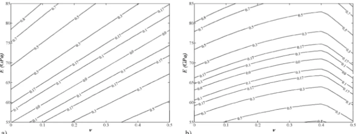
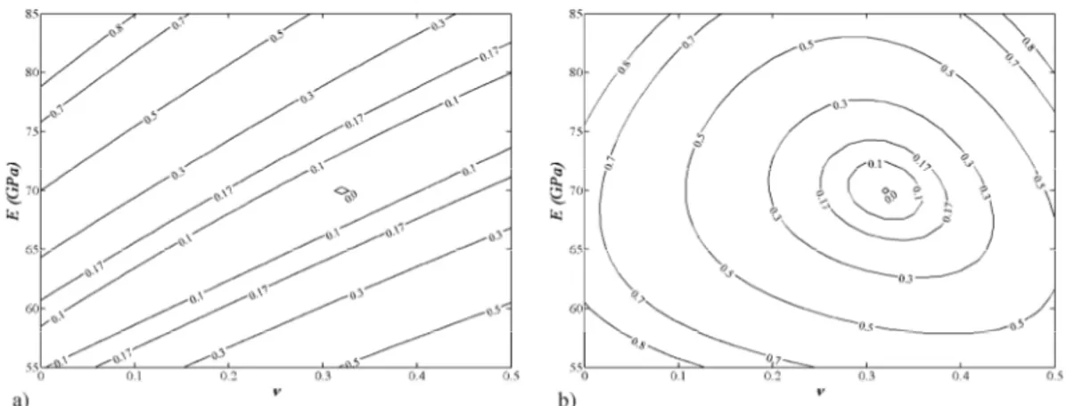
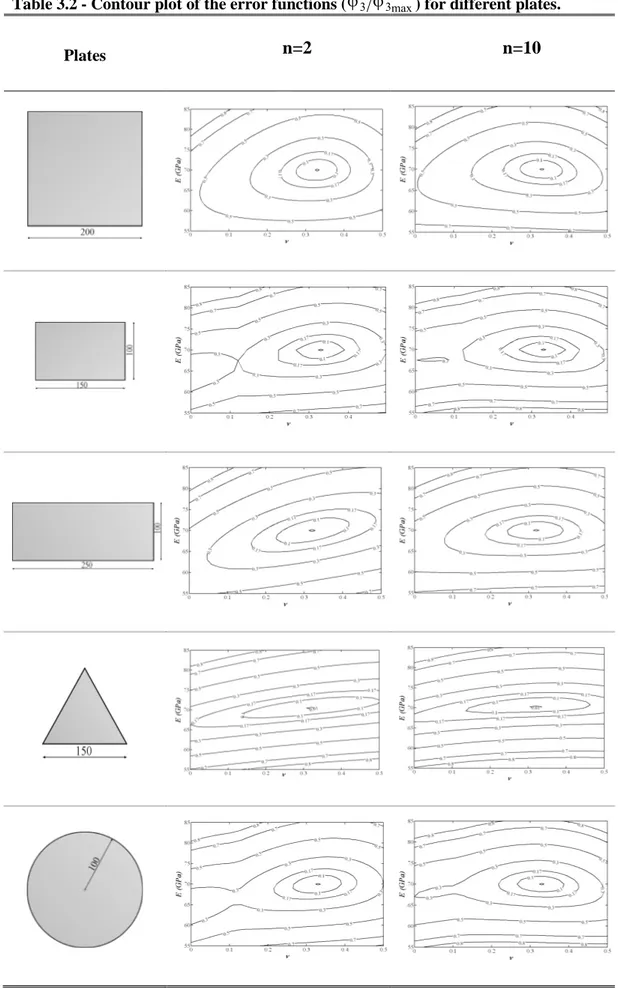
5.2.1 Error function and minimization method . . . . 5.3 Optimization of loading and constraining configuration . . . . 5.3.1 Plates of different shape . . . . 5.4 Numerical application and sensitivity analysis . . . . 5.5 Conclusion . . . . 5.6 Bibliography . . . . 105 105 107 108 111 121 122 125 126

(4)

Chapter 6

Experimental validation of the static technique . . . .

6.1 Introduction . . . . 6.2 Identification process . . . . 6.3 Experimental validation . . . . 6.4 Conclusion . . . . 6.5 Bibliography . . . . 130 130 131 132 142 142

Appendix A: Matlab code to acquire natural frequencies . . . . Appendix B: Genetic Algorithm code. . . . Appendix C: Interpolation procedure . . . .

147 155 172

(5)

I

NTRODUCTION

The elastic properties of solids play a fundamental role in both scientific and technological fields. Their measurement provides information regarding the forces exchanged among the atoms or ions that compose a solid, thus helping to characterise the nature of the links. It also allows us to describe the mechanical behaviour of the material which is fundamental for the structural design and experimental stress analysis. Moreover, the possibility of measuring the elastic constants of materials, fast and accurately, during the manufacturing cycle of a product could help with quality control. As a result there are many methodologies for the elastic characterization of materials. Today there is still great interest in this subject especially in the context of the development of new and more complex materials for which the classic methods of characterization appear time-consuming, expensive and, in some cases, unsuitable.

The increasing use of composite and ceramic materials in engineering has led to the development of new methodologies of characterization. Among these methodologies, the most promising are those identifying the elastic constants through a process that minimizes the difference between the dynamic or static response of the real structure (measured response) and the response of the same structure predicted by an analytical or numerical model (virtual response). These methods, known as mixed numerical-experimental techniques (MNET), update iteratively the values of the elastic constants of material in the model, until the virtual response (usually, the first natural frequencies in dynamic approaches or the field of superficial displacements or strains in static approaches) approximates as closely as possible the real response measured by means of experimental observations. The values of the constants used in the last iteration are the elastic properties of the material. The identification of all the elastic constants can take place simultaneously, with a single experiment and without damaging the specimen.

(6)

Introduction

Although such methodologies have been mainly devoted to the elastic characterization of anisotropic materials, where many elastic parameters are involved, they can certainly be used for the analysis of isotropic materials where only two parameters have to be identified. Indeed, many authors proved the effectiveness of their methodologies by analysing samples of isotropic materials with conventional geometrical shapes. However, there is no reason to think that the approach is unsuitable for characterizing specimens of different shape. Such a possibility could be very useful when the production of proper bulk specimens is not feasible or when the material sample must not be damaged or processed by a conventional testing geometry and therefore should be tested as it is.

The aim of the present work is the development of identification procedures to determine the elastic properties of isotropic and composite materials. The dissertation has been split into two part: the dynamic approach and the static approach. Due to the simplicity and the potentiality of the dynamic technique, in literature there are many works based on it, but, still today no one checked the feasibility and limits of its application to characterise isotropic plates (a more simple problem with only two elastic parameters) with geometry different from the standardised shapes. More specifically, the original contributions of this thesis to the dynamic field is the development and the application of the MNET to characterise isotropic plates of irregular shapes and layered materials. In particular, the Young modulus and Poisson ratio in a FE model of the specimen are updated until the corresponding first four natural frequencies match the experimental ones as closely as possible. For this purpose, different optimization methods and error functions have been compared in order to select the best combination of them. Furthermore, a numerical approach has been proposed to see the existence of a minimum in case of plates with a particularly complex shape. In addition, the dissertation suggests instrumentation and equipment for developing a cheaper and efficient measuring system. In the present thesis, the static way for the elastic characterization has been taken into account. As well as for the dynamic technique, a MNET has been applied to identify the elastic properties of isotropic or anisotropic materials. In this case, instead of the natural frequencies, the method makes use of the full-field measurement of the surface displacements of a plate of generic form under suitable flexural loads. The main advantage of the present identification method with respect to the traditional

(7)

Introduction

3 methodologies used for the characterization of unidirectional laminates is that all the elastic constants are determined from one static test. The original contributions of this thesis, in the static field, is the development of a correlation-based method to find the more suitable load and constrain configurations for any-shaped plates. This method is of great help in checking the feasibility of a specimen geometries for solving the elastic inverse problem by the full-field technique.

The thesis is composed of three main parts. The first part (chapters 1 and 2) gives an introduction to the elastic constant and to the standardised test methods present in literature. The second part (chapters 3 and 4) is related to the dynamic characterization; in particular the third chapter presents the theoretic aspects and the fourth ones provides the experimental validation and the practical aspects of the technique. The last part (chapter 5 and 6) is related to the static characterization: the fifth chapter provides a general overview of the proposed technique while the sixth chapter reports the experimental validation of the method.

(8)

1 L

INEAR ELASTICITY

1.1 The Generalized Hooke’s Law

The stress-strain relation that describes the linear elastic behaviour of a material can be expressed by matrices. The matrices take the name of compliance (S) or stiffness (C) matrices. The stiffness matrix is the inverse of the compliance matrix. The linear elastic stress-strain relation is given by the generalised Hooke’s law: σ ε ε σ S C   (1.1)

in which σ and ε represent the engineering stress and strain vector

respectively, expressed in a coordinate system parallel to the principal material axes. The stiffness matrix is used to find the stress field from the strain field, while the compliance matrix is used to find the strain field from the stress field. Since both σ and ε are vector with nine elements, the stiffness matrix S has to be 9×9 elements. This implies the need of 81 parameters to describe a material’s elastic stress-strain relation. In general, for a three dimensional anisotropic object the independent constants of the compliance matrix (S) are 21, while the non-zero elements of the matrices of elasticity are 36 (Gibson, 1994); this is due to the various symmetry conditions that simplify the equations. Both stresses and strains are symmetric due to equilibrium of an infinitesimal element, so that there are only six independent stress components and six independent strain components (minor symmetry). Furthermore, due to the existence of the strain energy density, the stiffness and compliance matrices are symmetric (main symmetry). Fortunately all the materials have some form of symmetry that can reduce the independent constants that describe the linear elastic behaviour, however, no known material is completely anisotropic (Gibson, 1994). For example, a

(9)

Chapter 1: Linear elasticity

5 monoclinic material has one plane of material property symmetry and so the number of independent moduli is reduced to 13. The orthotropic material has three orthogonal planes of material property symmetry, and in this case the number of independent elastic constants is reduced to 9. In this case, if the used coordinate system is not aligned with the principal material directions (the directions parallel to the intersection of the three orthogonal symmetry planes) the elastic matrices have 36 non-zero elements and the materials is called generally

orthotropic. If the used coordinate system is aligned with the principal material

directions (it is called principal or in-axis coordinate system) the elastic matrices have 12 non-zero elements and the materials is called specially orthotropic. In this last case the stiffness matrix becomes:

                     66 55 44 33 23 22 13 12 11 C 0 C SYM 0 0 C 0 0 0 C 0 0 0 C C 0 0 0 C C C C (1.2)

There is another kind of material symmetry that is important in the study of composites. In most composite materials the fiber-packing arrangement is statistically random in nature, so that the properties are nearly the same in any direction perpendicular to the fibers and the materials is called transversely

isotropic. In this last case the stress-strain behaviour can be described by 12

nonzero elastic moduli but only 5 are independent:

                     66 66 23 22 22 23 22 12 12 11 C 0 C SYM 0 0 )/2 C -(C 0 0 0 C 0 0 0 C C 0 0 0 C C C C (1.3)

where the 23 plane and all parallel planes are assumed to be planes of isotropy, and so that C12= C13, C22= C33 and C55= C66 and C44 is a function of the

(10)

If the material has an infinite number of symmetry planes, the material is said to be isotropic. In the case of an isotropic material the stress-strain behaviour can be described by 12 nonzero elastic moduli where only 2 are independent, in factC11= C22= C33, C12= C23= C13, C44=C55= C66=(C11-C12)/2and the relation becomes:

                     )/2 C -(C 0 )/2 C -(C SYM 0 0 )/2 C -(C 0 0 0 C 0 0 0 C C 0 0 0 C C C 12 11 12 11 12 11 11 12 11 12 12 11 C (1.4)

Table 1.1 reports the elastic coefficients in the stress-strain relationships for different materials and coordinate system.

Table 1.1 – Summary of the material symmetries.

Material and coordinate system Number of nonzero coefficients Number of independent coefficients Three-dimensional case Anisotropic 36 21 Generally Orthotropic (nonprincipal coordinates) 36 9 Specially Orthotropic (principal coordinates) 12 9 Specially Orthotropic Transverely isotropic 12 5 Isotropic 12 2 Two-dimensional case Anisotropic 9 6 Generally Orthotropic (nonprincipal coordinates) 9 4 Specially Orthotropic (principal coordinates) 5 4 Isotropic 5 2

Until now three-dimensional cases have been considered. Often some tension component can be neglected and so a two-dimensional cases can be obtained. In this case other simplification can be carried out and the matrices of elasticity become 3x3. If the material is anisotropic, the nonzero elements in the elastic matrices are 9 while the independent moduli are 6. If the material is

(11)

7 orthotropic and the off-axis coordinate system is considered, the nonzero elements are 9, while the independent moduli are 4. If an in-axis coordinate system is considered the nonzero elements become 5. For isotropic materials there are still 5 non zero elastic constants, but only 2 are independent

1.2 Engineering Constants

1.2.1 Isotropic Materials

In practice, elastic material properties are usually characterised with a set of engineering constants like generalised Young’s moduli, shear moduli and

Poisson’s ratios instead of the coefficients (Cij or Sij) of the elasticity matrices. The engineering constants are also widely used in analysis and design because they are easily defined and interpreted in terms of simple states of stress and strain (Timoshenko, Gere, 1997).

The assumption of the elasticity leads to the existence of a strain energy (U). For isotropic materials no preferential directions exist and so the stress-strain relation is independent of the coordinate system adopted for stress and strain description; in the elastic case this leads to the dependence of the strain energy (U) on the invariants (Corradi Dell’Acqua, 1992):

) I , I , I ( U d ) ( U ij ij ij ij 1 2 3 0  



    (1.5) with: ) det( I I I III II I I III III II II I III II I ε                     3 2 1 (1.6)

where I1, I2and I3 are the linear, quadratic and cubic invariants, whileI,II, IIIare the principal strains. In the linear caseUhas quadratic form, so that cubic

invariant does not exist in the energy expression:

2 2 1 bI

aI

U   (1.7)

where a and b are the constitutive parameters. Only two parameters are needed to describe the elastic linear stress-strain relation. The previous equation often is written using the Lamè constant (and G):

(12)

Chapter 1: Linear elasticity G b ) G ( a 2 2      (1.8)

Using Eq.(1.8)and Eq.(1.7)the expression of the strain energy became:

2 2 1 2 ) 2 ( 2 1 GI I G U 



  (1.9)

From the definition of the strain energy it is possible to obtain the following expression: ij ij U      _(1.10)

and so, using Eq.(1.9)and Eq.(1.10)it’s possible to write:

ij ij ij I G I I G







       1 2 1 2 ) 2 ( (1.11)

Unfortunately the Lamè’s constants are not easily defined and interpreted in terms

of simple states of stress and strain. As highlighted, usually, the elastic coefficients are expressed as a function of the so-called "engineering constants", which are more easily defined and interpreted in terms of simple states of stress and strain: ) ( 2 2 3 G G G G E           (1.12)

where E is the Young modulus (or modulus of elasticity), is the Poisson ratio and G is the shear modulus (or modulus of rigidity). Young’s modulus involves the longitudinal elongation of a material when it is subjected to a tension or compression test and it is defined as the ratio between the normal stress and the normal strain. The shear modulus implies the angular distortion undergone by the material when subjected to pure shear and it is defined as the ratio between the

shear stress and the shear strain. Finally, Poisson’s ratio describes the lateral (or

radial) contraction or expansion of the material when it is subjected to a longitudinal normal stress and is defined by the ratio between the strain in the lateral or radial direction and the strain in the longitudinal or axial direction.

(13)

9 Inverting the Eq.(1.12)it’s possible to obtain:

) 1 ( 2 ) 2 1 )( 1 (           E G E (1.13) (1.14)

Often the stress-strain relationship is written in terms of the three moduliE, and Gbut, it should be noted that, only two elastic constants are independent.

1.2.2 Orthotropic Materials

An orthotropic material can be characterised in three orthogonal directions

by twelve engineering constants. Considering a stress state where σiiis the only non-zero stress component, the Young’s modulus in the i-direction is defined as:

3 2 1 ,, i , E ii ii i  _   (1.15)

while the Poisson’s ratio for transverse strain in the j-direction when the material is stressed in the i-direction is defined as:

j i , , , j , i , ii jj ij  123    (1.16)

Note that, as with isotropic materials, a negative sign mast be used in the

definition of Poisson’s ratio.

The shear modulus in the ij-plane is defined as:

31 32 12, , ij , G ij ij ij _   (1.17)

considering a stress state whereijis the only non-zero stress component.

Since the engineering constants are defined for uni-axial stress conditions, it is much easier to express them in terms of compliance than in terms of stiffness. The combination of the definitions in Eqs. (1.15-1.17) with the strain-stress relations of an orthotropic material leads to the following compliance matrix:

(14)

Chapter 1: Linear elasticity                                          12 31 23 3 2 23 1 13 3 32 2 1 12 3 31 2 21 1 G 1 0 0 0 0 0 0 G 1 0 0 0 0 0 0 G 1 0 0 0 0 0 0 E 1 E ν E ν 0 0 0 E ν E 1 E ν 0 0 0 E ν E ν E 1 S (1.18)

The matrix shows 12 elastic constant. Due to the symmetry properties, only 9 moduli are independent, in fact it is possible to write:

j ji i ij E E    (1.19)

which means that there are only three independent Poisson’s ratios.

1.3 Constraints on the Engineering Constants

The elastic material parameters cannot take any value, they are restricted by a number of physical limits (Jones, 1999). The considered restrictions are the so-called thermodynamic constraints which are based on the principle that the total work done by all the stress components must be positive in order to avoid the creation of energy. The work done by a stress component is given by the product of the stress component with the corresponding strain component. The work of the stress components will only be positive, if the stiffness and compliance matrices are positive-defined.

1.3.1 Isotropic Materials

To have a positive work from the product of the tension and the longitudinal elongation, i.e. the Young modulus defined positive, the following inequality is necessary:

1

 

(15)

11 In the same way, if an isotropic material is subject to hydrostatic pressure (p), the volumetric deformation is:

B p ) ( / E p z y x    _        2 1 3 (1.21)

Where B is the Bulk modulus. To define B>0 the following relation are necessary: E > 0 2 1   (1.22) (1.23) 1.3.2 Orthotropic Materials

The restrictions on the orthotropic material parameters can be established using the same thermodynamic considerations as in the previous section: the total work done by all the stress components must be positive in order to avoid the creation of energy. It is possible to demonstrate (Jones, 1999) that this restriction, in the plane case, can be expressed by the following inequality:

0 1 0 0 0 21 12 12 2 1        G , E , E (1.24)

UsingEq.(1.19) it is possible to obtain:

1 2 21 2 1 12 E E or E E     (1.25)

1.4 Elastic Properties for an Arbitrary Orientation

For plate-like structures, the stress analysis is usually carried out under the Kirchhoff assumptions. For a structure parallel to the 12-plane, the Kirchhoff

assumptions result in plane stress state (σ3 = 0, τ23 = 0, τ31 = 0). Accepting the Kirchhoff assumptions, the general strain-stress relation for specially orthotropic materials reduces to the following in-plane strain-stress relation:

(16)

Chapter 1: Linear elasticity                                12 2 1 66 22 21 12 11 12 2 1 0 0 0 0       S S S S S (1.26)

where the compliance coefficients Sij and the engineering constants are related to each other by the following equations:

12 66 2 21 1 12 21 12 2 22 1 11 1 1 1 G S , E E S S , E S , E S           (1.27)

The lamina stresses in terms of tensor strains are given by:

                               12 2 1 66 22 21 12 11 12 2 1 0 0 0 0       Q Q Q Q Q (1.28)

where the stiffness coefficients Qij are referred to the plane stress-reduced stiffness because they are obtained from Cij. They are related to the engineering constants in the following manner:

12 66 66 21 12 2 2 12 22 11 11 22 21 21 12 2 12 2 12 22 11 12 12 21 12 1 2 12 22 11 22 11 1 1 1 1 G S Q E S S S S Q C E S S S S Q E S S S S Q                        (1.29)

The properties described in Eq. (1.26) are defined in the directions of the principal material axes. These on-axis properties describe the behaviour of the material when subjected to a stress field that is aligned with the principal material axes (1-2), but this behaviour can vary with the orientation of the considered load. As with isotropic materials, a normal stress induces only normal strains, and all shear strains are equal to zero. This lack of shear/normal interaction is observed only for the principal material coordinate system. For any other set of coordinates the so-called “shear-coupling” effect is present. The off-axis properties describe the material behaviour when subjected to a stress field with an

(17)

13 arbitrary orientation (x-y). Consider a load with an arbitrary orientation and a global axis system x-y which is aligned with the principal directions of this load. In this local axis system, the stress-strain relation can be expressed as:

 

 

 

C

 

 (1.30)                                xy y x xy y x Q Q Q Q Q Q Q Q Q       66 26 16 26 22 12 16 12 11 (1.31)

where the overbars indicate that the quantities are expressed in local coordinates (off-axis properties). The transformed stiffness matrix

 

C contains the off-axis properties. The off-axis properties can be obtained starting from the on-axis properties in the following way:

 

Q 

    

T 1 Q T (1.32)

where [T] is the transformation matrix defined as (Tsai and Hahn, 1980):

                            2 2 2 2 2 2 2 2 sin cos sin cos sin cos sin cos cos sin sin cos sin cos T (1.33)

whereis the angle between the x- and 1-axis, as shown in Figure 1.1.

Figure 1.1 - Definition of the orientation angle θ.

Note that, for an arbitrary value of the orientation angle θ, the transformed compliance matrix has nine non-zero elements. However, the elastic behaviour is still fully characterized by only four independent material constants.

It is possible to obtain the same relation for the compliance when a global axis system x-y is considered:

(18)

 

 

 

S

 

 (1.34)                                xy y x xy y x S S S S S S S S S       66 26 16 26 22 12 16 12 11 (1.35)

where the S_ijare the components of the transformed lamina compliance matrix which are defined as follows:















S 2S S S (S 2S S S )cos4θ



2 1 S sin2θ )cos2θ S S S 2 (S S S 2 1 S sin2θ )cos2θ S S S 2 (S S S 2 1 S θ θcos )sin S (2S θ cos S θ sin S S )cos4θ S S S 2 (S S S S 6 S 8 1 S θ θcos )sin S (2S θ sin S θ cos S S 66 22 12 11 66 22 12 11 66 66 22 12 11 22 11 26 66 22 12 11 22 11 16 2 2 66 12 4 22 4 11 22 66 22 12 11 66 22 12 11 12 2 2 66 12 4 22 4 11 11                                     (1.36)

The lamina engineering constants can also be transformed from the principal material axes to the off-axes coordinates. For example, the modulus of elasticity associated whit uniaxial loading along the x direction is defined as:

11 11 1 S S E x x x x x  _     (1.37)

where the strain x in the denominator has been found by substituting the stress conditionx≠0,y=y=0. By replacing S11and using Eq.(1.27)it is possible

to write:      4 2 2 2 12 1 12 4 1 1 1 2 1 1 sin E sin cos G E cos E E_x            (1.38)

Similar transformation equations may be found for other off-axis engineering constants such as vxy and Gxy (Gibson, 1994) replacing the Sijin the following equations:

(19)

Chapter 1: Linear elasticity 15 66 0 σ σ xy xy xy 22 12 0 τ σ y x yx 11 12 0 τ σ x y xy 22 0 τ σ y y y 11 0 τ σ x x x S 1 γ τ G S S ε ε ν S S ε ε ν S 1 ε σ E S 1 ε σ E y x xy x xy y xy x xy y                       (1.39)

The variation of these properties with lamina orientation for a fiber-reinforced composite (E1=100 GPa, E2=10 GPa, G12=6 GPa and12=0.3) is shown graphically in Figure 1.2. As intuitively expected, Ex varies from a maximum at

= 0° to a minimum at= 90° for this particular material.

Figure 1.2 – Variation of lamina engineering constant with lamina orientation.

The shear-coupling effect has been described previously as the generation of shear strains by off-axis normal stresses and the generation of normal strains by off-axis shear stresses. To quantify the degree of shear coupling a dimensionless shear-coupling ratio may be defined (Halpin, 1984). There are two ways to define it. For example, when the state of stress is defined asx≠0,y=y=0, the ratio

11 16 S S x xy xy , x      (1.40)

is a measure of the amount of shear strain generated in the xy plane per unit normal strain along the direction of the applied normal stressx.

Other shear-coupling ratios can be defined for different states of stress. For example, when the stresses arey≠0,y=x=0, the ratio

(20)

Chapter 1: Linear elasticity 66 26 S S xy y y , xy     (1.41)

characterizes the normal strain response along the y direction due to a shear stress in the xy plane.

In the same way, other shear-coupling ratios can be defined as:

22 26 S S y xy xy , y      (1.42) 66 16 S S xy x x , xy  _    (1.43)

As shown in Figure 1.3, _x_,_xystrongly depends on orientation and has its maximum value at some intermediate angle.

Figure 1.3 – Variation of the shear-coupling ratios.

1.5 The classical laminated plate theory

In general, the composite materials are manufactured in the form of thin sheets, called laminae or layers. These sheets present a low stiffness. In order to increase the stiffness of the component, laminae are bonded together to form a laminate. In composite manufacturing exist a number of design parameters like:

1. layer materials 2. layer orientation 3. number of layers 4. layer thickness

(21)

17 In most applications, the thickness of a laminate is small compared to the planar dimensions, so that two-dimensional theories can be used to analyse composite laminates. Two-dimensional theories are obtained from the three-dimensional elasticity theory by making assumptions concerning the variation of displacements and/or stresses through thickness of the laminate. The classical laminated plate theory (CLPT) is an extension of the classical plate theory to laminated plates. In this theory, the in-plane displacements are assumed to vary linearly through the thickness and the transverse displacement is assumed to be constant through the thickness (i.e., transverse normal strain is zero). The classical laminated plate theory is found to be adequate for most applications where the thickness of the laminate is two orders of magnitude smaller than the in-plane dimensions. When the classical laminated plate theory is not applicable, a refined theory is used. A refinement to the classical laminate theory is provided by the first-order shear deformation plate theory (FSDT) (Reddy, 1992).

Figure 1.4 – Coordinate system and stress resultants for laminated plate

Although the laminate is made up of multiple laminae, it is assumed that the individual laminae are perfectly bonded together so as to behave as a unitary, nonhomogeneous, anisotropic plate. Interfacial slip is not allowed and the interfacial bonds are not allowed to deform in shear, which means that displacements across lamina interfaces are assumed to be continuous. These assumptions mean that the deformation hypothesis from the classical homogeneous plate theory can be used for the laminated plate. Figure 1.4 defines the coordinate system to be used in developing the laminated plate analysis. The xyz coordinate system is assumed to have its origin on the middle surface of the plate, so that the middle surface lies in the xy plane. The displacements at a point

(22)

in the x, y, z directions are u, v, and w, respectively. The basic assumptions relevant to the present static analysis are (Gibson, 1994):

1. The plate consists of orthotropic laminae bonded together, with the principal material axes of the orthotropic laminae oriented along arbitrary directions with respect to the xy axes;

2. The thickness of the plate, t, is much smaller than the lengths along the plate edges a and b;

3. The displacements u, v, and w are small compared with the plate thickness. 4. The in-plane strains εx, εy,and γxyare small compared with unity;

5. Transverse shear strains γxzand γyzare negligible;

6. Tangential displacements u and v are linear functions of the z coordinate; 7. The transverse normal strain εzis negligible;

8. Each ply obeys Hooke's law; 9. The plate thickness t is constant;

10. Transverse shear stresses τxz and τyz vanish on the plate surface defined by

z = ±t/2.

Assumption 5 is a result of the assumed state of plane stress in each ply, whereas assumptions 5 and 6 together define the Kirchhoff deformation hypothesis that normals to the middle surface remain straight and normal during deformation. According to the previous assumptions, the displacements can be expressed as: ) , ( ) , ( ) , ( 0 0 0 y x w w y w z y x v v x w z y x u u          (1.44)

from which it is possible to find the strain:

y x w z x v y u z y w z y v z x w z x u z                             2 0 0 xy 0 xy xy 2 2 0 y 0 y y 2 2 0 x 0 x x 2 κ γ γ κ ε ε κ ε ε (1.45)

(23)

19 where u0, v0 and w0 are the displacements of the middle surface, x is a

bending curvature associated with bending of middle surface in the xz plane and

y is a bending curvature associated with bending of middle surface in the yz

plane. xy is a twisting curvature associated with out-of-plane twisting of the

middle surface which lies in the xy plane before deformation.

Using Eq. (1.45)and Eq. (1.31)it is possible to find the stress along arbitrary

xy axes in the k-th lamina of a laminate:

                                  xy xy y y x x k k xy y x z z z Q Q Q Q Q Q Q Q Q          0 0 0 66 26 16 26 22 12 16 12 11 (1.46)

From this equation it is possible to note the shear-coupling effect due to the anisotropic behaviour of the off-axis lamina.

In the laminated plate analysis Eq. (1.46) for lamina stress is of limited practical use because the curvatures are not generally known and are difficult to measure. Thus, the midplane strains and curvatures can be related to applied forces and moments by static equilibrium equations in order to make these equations more useful. In the laminated plate analysis, however, it is convenient to use forces and moments per unit length rather than forces and moments. The forces and moments per unit length shown in Figure 1.4 are also referred to as stress resultants.

For example, the force per unit length, Nij, and the moment per unit length

Mijare given by:

 









 _  _     2 2 k 1 k ij ij ij 2 2 k 1 k ij ij ij σ σ M σ σ N t t N _z z t t N _z z k 1 -k k 1 -k dz z dz z dz dz (1.47)

where N is the number of layers in the laminate, and (zk,zk+1) are the thickness

coordinates of the bottom and top of thek-th layer.

(24)

Chapter 1: Linear elasticity                                                                         xy y x 0 xy 0 y 0 x 33 23 13 33 23 13 23 22 12 23 22 12 13 12 11 13 12 11 33 23 13 33 23 13 23 22 12 23 22 12 13 12 11 13 12 11 xy y x xy y x κ κ κ γ ε ε D D D B B B D D D B B B D D D B B B B B B A A A B B B A A A B B B A A A M M M N N N M N  (1.48)

where the elements of the matrix A, B and D are defined as:













                  N k z z k ij / t / t ij k N k z z k ij / t / t ij k N k k k k ij / t / t ij k ) z z ( ) Q ( dz z ) Q ( ) z z ( ) Q ( dz z ) Q ( ) z z ( ) Q ( dz ) Q ( 1 3 1 3 2 2 2 ij 1 2 1 2 2 2 ij 1 1 2 2 ij 3 1 D 2 1 B A (1.49)

From Eq. (1.48) it is possible to note that the extensional stiffness matrix A relates the in-plane forces {N} to the midplane strains {°} and the bending stiffness matrix D relates the moments {M} to the curvatures {k}. The coupling stiffness matrix B couples the in-plane forces {N} with the curvatures {k} and the moments {M} with the midplane strains {°}. A laminate having nonzero Bijwill bend or twist under in-plane loads. Such a laminate will also exhibit midplane stretching under bending and twisting moment loading. It can be easily shown that laminate geometric and material property symmetry with respect to the middle surface leads to the condition that all Bij= 0 and that asymmetry about the middle surface leads to nonzero Bij. Note that there are two types of coupling: the lamina shear coupling, that it is a result of anisotropic material behaviour, and the laminate shear coupling, that it is due to geometric and/or material property asymmetry with respect to the middle surface and is unrelated to material anisotropy.

The laminate Force-Deformation equation described by the matrices A, B and D can be inverted. The inverted equations are described by other three matrices A’, B’ and D’. When the coefficient of the matrix B’ are zero, A’ is also used in the derivation of the effective laminate engineering constants:

(25)

Chapter 1: Linear elasticity 21 33 xy 22 12 yx 11 12 xy 22 y 11 x A' 1 G A' A' ν A' A' ν A' 1 E A' 1 E h h h       

Using similar derivation, effective laminate flexural moduli may be expressed in terms of the flexural compliances (Dij’):

33 3 fxy 22 12 fyx 11 12 fxy 22 3 fy 11 3 fx D' 12 G D' D' ν D' D' ν D' 12 E D' 12 E h h h        .

1.6 Bibliography

Corradi Dell’Acqua, L., 1992. Meccanica delle strutture. McGraw-Hill libri, Italia

Gibson, R.F., 1994. Principles of Composite Material Mechanics. McGraw Hill, Singapore.

Halpin J.C., 1984. Primer on composite materials: analysis. Technomic Publishing Co., Lancaster.

Jones R. M., 1999. Mechanics of Composite Materials, Taylor & Francis, Philadelphia.

Reddy, J.N., OCHOA, O.O., 1992. Finite Element Analysis of Composite Laminates. Kluwer Academic Publishers, London.

Timoshenko S.P., Goodier J.N., 1970. Theory of Elasticity. McGraw Hill, New York.

Timoshenko S.P., Gere J.M., 1997. Mechanics of Materials, PWS Publishing Company, Boston.

Tsai S.W., Hahn H.T., 1980. Introduction to Composite Materials. Technomic Publishing Co., Lancaster.

(26)

2 S

TANDARD TEST METHODS FOR

THE ELASTIC CHARACTERIZATION

OF MATERIALS

2.1 Introduction

The knowledge of the elastic properties of materials is very important for both structural design and engineering applications and the possibility of measuring them, fast and accurately and during the production process, could be a valid improvement for quality control. Because of such importance, the great number of methodologies developed and presented in the scientific literature is not surprising. Still today, the argument gives rise to a wide interest among researchers, especially in the context of the development of new and more complex materials, for which the classical methods of characterization appear slow, expensive and not always suitable.

The methods for determining the elastic properties of a materials can be classified into two big categories: static methods and dynamic methods. Static methods are generally based on direct measurement of strains and stress components of a suitable specimen subject to mechanical test (tensile, compressive, flexural, torsional, etc.). Young and shear moduli are determined from the slope of the linear region of the stress–strain curve, while Poisson’s ratio is determined from the ratio between transverse and longitudinal strains of a specimen loaded by a uniaxial load (Carlsson and Pipes, 1997). The elastic moduli influence the dynamic behaviour of the material (for example, its mechanical resonant frequencies or the sound velocity); so that, such properties can be used in order to characterise a suitable test specimen. Dynamic methods are generally based on this principles. In the present chapter a review of both the basic static and dynamic standard test for determining the elastic constant of materials are

(27)

Chapter 2: Standard test methods for the elastic characterization of materials

23

2.2 Dynamic procedures

Starting from 1935, when the first dynamic characterization applications have been carried out, the dynamic technique have grown into valid tools for measuring the elastic moduli of isotropic materials. In standardised resonant methods, Young's modulus, shear modulus, and Poisson's ratio can all be computed from the resonant frequencies of prismatic bars, rods, or slabs. There are several ASTM standards that cover the determination of elastic properties of specific materials by measuring resonance frequencies by sonic resonance or by impulse excitation of vibration. All these test methods may differ from each other in several areas (e.g., sample size, dimensional tolerances, sample preparation).

The ASTM C848 (“Young’s Modulus, Shear Modulus, and Poisson’s Ratio For Ceramic Whitewares by Resonance”) allows to obtain the elastic properties of

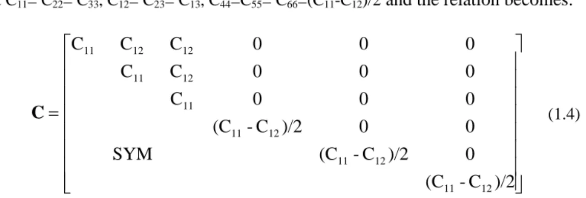
ceramic materials using the sonic resonance. In fact, this test method measures the resonance frequencies of test bars of suitable geometry by exciting them at continuously variable frequencies. Mechanical excitation of the specimen is provided through a transducer that transforms an initial electrical signal into a mechanical vibration (see Figure 2.1). Another transducer senses the resulting mechanical vibrations of the specimen and transforms them into an electrical signal that can be displayed on the screen of an oscilloscope to detect resonance. In the end, the resonance frequencies, the dimensions, and the mass of the

specimen are used to calculate Young’s modulus and the shear modulus.

Figure 2.1 – Specimen Positioned for Measurement of Flexural and Torsional Resonance Frequencies Using “Tweeter” Exciter (extracted from the ASTM C848)

ASTM C1198 describes a test method for determining the dynamic elastic module of advanced ceramics. It is a clone of two earlier ASTM standards (C848 and C623) and, rather than using the tables and graphs (like in the previous standards), uses the original equations for relating the elastic constants to the resonance frequencies. Although recommended sizes for flat and round specimens

(28)

are given, the equations are sufficiently general, so that a wide size range can be used. The equations include the conventional polynomial correction factors to reflect the finite specimen thicknesses, but simplified equations are also provided for instances where the length-to-thickness ratio of the specimens is greater than 20. ASTM standards C1198 and C1259 form the basis for two ASTM standards:

ASTM E1875 (“Standard Test Method for Dynamic Young's Modulus, Shear Modulus, and Poisson's Ratio by Sonic Resonance”) and ASTM E1876 (“Standard Test Method for Dynamic Young's Modulus, Shear Modulus, and Poisson's Ratio by Impulse Excitation”). These two standards are identical

versions of C1198 and C1259, which are generic and are not confined to ceramic materials, but are applicable to all elastic materials. The ASTM standard C1259 allows to derive the elastic properties of homogeneous isotropic materials measuring the resonant frequencies of beam-shaped specimen with rectangular cross-section by exciting it mechanically by a singular elastic strike with an impulse tool (instead of using the sonic resonance as in the C1198 and in the E1875). A transducer (for example, a contact accelerometer or a non-contacting microphone) senses the resulting mechanical vibrations of the specimen and transforms them into electric signals (see Figure 2.2). Specimen supports, impulse locations, and signal pick-up points are selected to induce and measure specific modes of the transient vibrations. The signals are analyzed, and the fundamental resonant frequency is measured.

Figure 2.2 – Block Diagram of Typical Test Apparatus (extracted from the ASTM C1259)

The appropriate fundamental resonant frequencies, dimensions, and mass of the specimen are used to calculate dynamic moduli. In particular, the elastic modulus can be derived from the fundamental out-of-plane flexural vibration mode using the following equation:

(29)

Chapter 2: Standard test methods for the elastic characterization of materials 25 1 3 3 2 9465 0 T t L b mf . E f (2.1)

where b, L, t are the width, the length and the thickness of the beam, while ffis the

fundamental natural frequencies and m is the mass. T1 is a correction factor

defined as:                                                2 2 4 2 4 2 2 1 ) 536 1 1408 0 1 ( 338 6 00 1 ) 173 2 2023 0 1 ( 340 8 868 0 ) 8109 0 0752 0 1 ( 585 6 1 L t . . . . L t . . . L t . L t . . . T       (2.2)

The shear modulus can be obtained using the following equation

A B bt mLf G t   1 4 2 (2.3)

where ftis the torsional vibration frequency, while A and B are given as follows:

                                                   2 3 2 892 9 03 12 0078 0 3504 0 8076 0 5062 0 t b . t b . t b . t b . t b . . A (2.4)                                   ₂ ₃ 21 0 52 2 4 b t . b t . b t b t t b B _(2.5)

When L/t20 Eq. (2.2) can simplified to the following form:

2 585 6 1 1         L t . T (2.6)

Therefore from Eqs. (2.3) and(2.5) is possible to calculate both E and G. If

, t /

L 20 the elastic modulus has to be calculated with an estimation of the Poisson ratio and an iterative procedure.

In the ASTM E1876 there is an annex that covers the evaluation of the frequencies of disc geometry specimens for the determination of the dynamic elastic properties of elastic materials at ambient temperatures. With a disc-shaped

(30)

specimen, the Poisson’s ratio is determined using the first two resonant frequencies. The dynamic Young’s modulus and dynamic shear modulus are then calculated using the Poisson’s ratio, the experimentally-determined fundamental

resonant frequencies, and the specimen dimensions and mass.

The fundamental equation defining the relationship between the natural resonant frequency, the material properties, and the specimen dimensions can be found on the ASTM standards and is defined as:

h A r K f i i   2  (2.7)

where fi is the resonant frequency of interest, Ki is the geometric factor for

that resonant frequency, r is the radius of the disc,is the density of the disc and

A is the plate constant defined as:

) ( Eh A ₂ 3 1 12   (2.8)

where t is the disc thickness, E is Young’s modulus and  is the Poisson’s

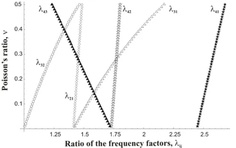
ratio for the disc material. This is a general equation which is valid for both the first and the second natural vibrations. Poisson’s ratio can be determined directly from the experimental values of the first and the second natural resonant frequency by the use of suitable tables present on the ASTM E1876. The value for

Poisson’s ratio is interpolated from the table using the ratio of the second natural

resonant frequency to the first natural resonant frequency (f2/f1) correlated with the

ratio of the specimen thickness to the specimen radius (t/r). For the Young’s modulus of a disc, two calculations of E (E1and E2) are made independently from

the two resonant frequency measurements, and then a final value E is determined by averaging the two calculated values:

2 1 699 37 1 699 37 2 1 3 2 2 2 2 2 2 2 3 2 1 2 2 2 1 1 E E E t K ) ( m D f . E t K ) ( m D f . E         (2.9)

Unfortunately all these dynamic standards cannot be applied to the orthotropic materials and an extension seems not easy to carry out. This is due

(31)

27 mainly to the difficulty of finding a fundamental equation that describes the dynamic behaviour of these materials.

2.3 Static procedures

Considering the stress state imposed to the specimen, the static methods can be classified in the following groups:

 Tension Test Methods

 Compressive Test Methods

 Flexure Test Methods

 Shear Test Methods

In theory, to characterise an isotropic material only the stress-strain state in a point of the sample is necessary; the simplest way to develop this is to test the sample in tension with a known load and measuring the strain by one or more strain-gages. The physics of composites testing may appear to be similar to the physics of testing isotropic materials, but the differences are significant. Determination of the mechanical behaviour is influenced by several factors that include metallurgical/material variables, test methods, and the nature of the applied stresses. The properties of a test sample made of composite materials are often significantly different in different directions; consequently, special testing methods may be required (ASM Vol. 21). For example, uniaxial mechanical tests never produce a pure uniaxial stress state throughout an entire test specimen; three dimensional stresses always exist at discontinuities and loading points. Many isotropic materials are created as bulk material and later formed into the end product. However, most composites are consolidated into the final material form at the same time that the end product is produced. This can introduce additional process variations into the basic material.

The tension test is one of the most commonly used tests for evaluating

materials. In its simplest form, the tension test is carried out by gripping opposite ends of a sample within the load frame of a test machine. A tensile force is applied by the machine, resulting in the gradual elongation and eventual fracture of the sample. During this process the force-extension data are monitored and recorded. When properly conducted, the tension test provides force extension data that can quantify several important mechanical properties of a material like the

(32)

elastic deformation properties (such as the modulus of elasticity and Poisson's ratio), the yield strength, the ultimate tensile strength and the ductility properties (such as elongation). The ASTM E111 describes the method for the determination

of Young’s modulus, tangent modulus, and chord modulus of isotropic materials

by tension test. The tangent modulus is the slope of the stress-strain curve at a specified value of stress or strain while the chord modulus is the slope of the chord drawn between any two specified points on the stress-strain curve, below the elastic limit of the material. These two moduli are used for materials that follow nonlinear elastic stress-strain behaviour. Furthermore the standards give the recommendation on the preparation of specimens, the temperature control, the speed of testing, the alignment of the sample into the test machine etc. In ASTM E132 the value of Poisson’s ratio is obtained from the longitudinal and the transverse strains resulting from uniaxial stress only at room temperature. This test method is limited to specimens of rectangular section and to materials in which creep is negligible compared to the strain produced immediately upon loading.

The general concept of tensile properties is very similar for metallic and non-metallic materials, but there are also some differences in their behaviour and so in the required test procedures. Ceramics materials are brittle materials that are extremely sensitive to bending strains, besides the hard surface of ceramics reduces the effectiveness of frictional gripping devices; so that tension testing of ceramics requires more attention to alignment and gripping of the sample in the test machine. The procedure to apply tension testing to monolithic ceramics at room temperature is described in ASTM standard C1273 (“Test Method for Tensile Strength of Monolithic Advanced Ceramics at Ambient Temperatures”), while the standard method for continuous fiber-reinforced advanced ceramics at ambient temperatures is described in C1275 (“Test Method for Monotonic Tensile Behaviour of Continuous Fiber-Reinforced Advanced Ceramics with Solid Rectangular Cross-Section Test Specimens at Ambient Temperature”). Plastic materials are viscoelastic materials that exhibit time-dependent deformation during force application and so the tension depend more strongly on the strain rate and on the temperature. Thus, control of temperature and strain rates are more critical than for metals. The ASTM standard D638 (“Test Method for Tensile Properties of Plastics”) describes the tension test for unreinforced and reinforced

(33)

29 plastic materials and includes the option of determining Poisson’s ratio at room temperature; for tensile properties of resin-matrix composites reinforced with oriented continuous or discontinuous high modulus (more than 20GPa) fibers, tests shall be made in accordance with Test Method D3039/D3039M (“Standard

Test Method for Tensile Properties of Polymer Matrix Composite Materials”).

The standard reports all the recommendations for the specimen design tolerances, control of test machine-induced misalignment and bending, measurement of thickness, selection of transducers and calibration of instrumentation, description of failure modes and the definition of elastic property calculation. The Test Method ISO 527 is substantially based on ASTM D3039, but this last standard offers better control of testing details that may cause variability and, for this reason, is the preferred method. By changing the sample configuration, the tensile test methods are able to evaluate different material configurations, including unidirectional laminates, woven materials, and general laminates. However, some sample-material configuration combinations are less sensitive to specimen preparation and testing variations than others. Perhaps the most dramatic example is the unidirectional specimen. Fiber versus load axis misalignment in a 0° unidirectional specimen, which can occur due to either specimen preparation or testing problems or both, can reduce strength as much as 30% due to an initial 1° misalignment (ASM Vol. 21). Furthermore, bonded end tabs can actually cause premature failure of the sample (even in nonunidirectional case) if not applied and used properly. The characterization of composite is not easy due to the mentioned problem and similar issues.

Figure 2.3 – End tabs used in tension test

In each of the previous test methods, a tensile stress is applied to the specimen through a mechanical shear interface at the ends of the specimen, normally by either wedge or hydraulic grips. If used, the end tabs are intended to distribute the load from the grips to the specimen with a minimum of stress concentration. Tabs should be made from [±45°] or [0/90°] glass/epoxy or woven fabric composites and they are bonded on each side of the specimen. The load is

(34)

transferred into the specimen test section through shear (see Figure 2.3). The material response is measured in the gage section of the coupon by either strain gages or extensometers, subsequently determining the elastic material properties. In Figure 2.4 a typical specimen is reported, while in Table 2.1 the recommended specimen dimensions are reported.

Figure 2.4 Tension test specimen

Table 2.1 –Tensile specimen geometry recommendations (ASTM D3039) Fiber

Orientation Width

Overall

Length Thickness Tab Length

Tab Thickness

[mm] [mm] [mm] [mm] [mm]

0° unidirectional 15 250 1.0 56 1.5

90° unidirectional 25 175 2.5 25 1.5

balanced and symmetric 25 250 2.5 emery cloth —

random-discontinuous 25 250 2.5 emery cloth —

To characterize the tensile response of unidirectional lamina, 0° and 90° specimens are employed to determine longitudinal and transverse properties. The [±45°] laminate tension test measures shear properties of the lamina. If Poisson's ratio is desired, a 0/90° strain gage rosette should be bonded in the center-gage-section region of the specimen. The properties obtained from tension tests on composite materials are effective (average) properties. The test method applies to unidirectional composites but can also be performed on laminates, woven fabrics, or discontinuous fiber composites. For asymmetric and/or unbalanced laminates, extension/bending coupling and extension/shear coupling effects produce nonuniform stress states in the test section. Obviously, under these conditions, effective properties cannot be accurately determined from the tensile test.

(35)

31

The compression test is conducted on composite materials, using appropriate

instrumentation, to determine compressive modulus, Poisson's ratio, ultimate compressive strength or strain-at-failure. These properties are determined through the use of test fixturing that is typically designed to be as simple to use and fabricate as possible, to minimize stress concentrations, to minimize specimen volume, and to introduce a uniform state of uniaxial stress in the specimen test section. Several compression test methods emerged during the past twenty years, and much confusion exists on their relative virtues. The numerous compression test methods available can be broadly classified into three groups based on load introduction and specimen design: shear loading, end-loading, and sandwich beam specimen testing (see Figure 2.5).

a) b) c)

Figure 2.5 - Generic types of compression test methods. (a) Shear loaded. (b) End-loaded. (c) Sandwich beam (extracted from the ASM Vol. 8)

The measured compression strength for a single material system has been shown to differ when determined by different test methods. Variation in results can usually be attributed to fabrication practices, control of fiber alignment, improper specimen preparation and machining, improper placement of samples in testing machines, and improper use of test equipment. Sufficient restraint must be provided to inhibit undesirable failure modes, such as column buckling of the sample. However, if excessive restraint is used, the resulting failure strengths may be artificially high. Buckling and kinking of the fibers within the composite are features regarded as representative for the material and should not be inhibited. To avoid buckling instability, relatively short gage lengths are necessary, but short gage lengths generally tend to amplify sensitivities to clamping. Thus, for very short gage lengths, the apparent compressive strength tends to decrease.

(36)

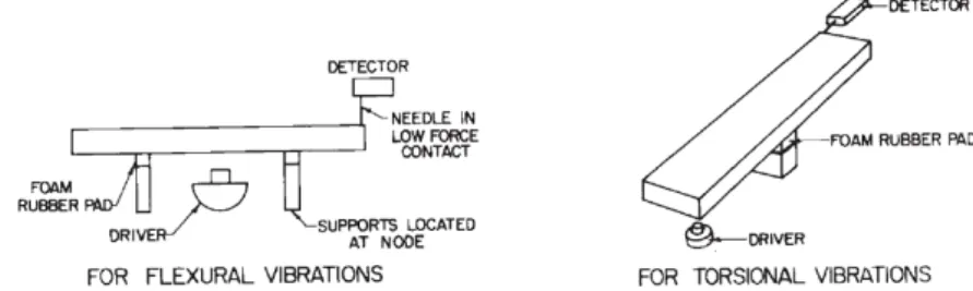
The ASTM D3410 (“Test Method for Compressive Properties of Polymer Matrix Composite Materials with Unsupported Gage Section by Shear Loading”) covers the determination of the in-plane compressive properties of polymer matrix composite materials reinforced by high-modulus fibers. The composite material forms are limited to continuous-fiber or discontinuous-fiber reinforced composites for which the elastic properties are specially orthotropic with respect to the test direction. This test procedure introduces the compressive force into the specimen through shear at wedge grip interfaces. Since the compressive load is introduced in the specimen through shear via tabs, there are stress concentrations in the regions at the ends of the end tabs at the beginning of the gage section. Consequently, failures are commonly observed close to the ends of the end tabs, but, such failures are difficult to avoid and are commonly accepted. In Figure 2.6 an example of common failure modes are reported.

Acceptable Failure Modes Unacceptable Failure Modes

Figure 2.6 - Sketch of the specimen failure (extracted from ASTM D3410)

The ASTM D695 (“Standard Test Method for Compressive Properties of

Rigid Plastics”) covers the determination of the mechanical properties of

unreinforced and reinforced rigid plastics, including high-modulus composites, when loaded in compression at relatively low uniform rates of straining or loading. This test procedure introduces the compressive force into the specimen by end-loading.

The ASTM D6641/D6641M (“Determining the Compressive Properties of Polymer Matrix Composite Laminates Using a Combined Loading Compression

(37)

33 (CLC) Test Fixture”) method establishes a procedure for determining the compressive strength and stiffness properties of polymer matrix composite materials using a combined loading compression or comparable test fixture. The compressive force is introduced into the specimen by combined end- and shear-loading. This test method is applicable to general flat laminates that are balanced and symmetric and contain at least one 0° ply. Unidirectional (0° ply orientation) composites can be tested to determine unidirectional composite modulus and

Poisson’s ratio.

The ASTM D5467 (“Compressive Properties of Unidirectional Polymer Matrix Composites Using a Sandwich Beam”) uses a honeycomb-core sandwich beam that is loaded in four-point bending, placing the upper face-sheet in compression (see Figure 2.7). The upper sheet is loaded in compression and is usually a six-ply unidirectional laminate. The lower face-sheet is typically the same material, but twice thicker in order to drive failure into the compressive face-sheet. The two face-sheets are separated by and bonded to a deep honeycomb core (usually aluminium). Failure of the compressive face-sheet enables measurement of compression strength, compression modulus, and strain-at-failure if strain gages or extensometers are employed. This procedure is applicable primarily to laminates made from prepreg or similar product forms. Other product forms may require deviations from the test method.

Figure 2.7 - Longitudinal compression sandwich beam test specimen.

ASTM C393 (“Flexural Properties of Flat Sandwich Constructions”) is one of a series designed to test sandwich constructions, and covers the determination of the properties of flat, sandwich constructions subjected to flatwise flexure in the same manner as ASTM D5467. ASTM C393 expands on the properties measured by ASTM D5467, and provides a methodology to determine the flexural