POLITECNICO DI MILANO
Facoltà di Ingegneria Industriale
Corso di Laurea Magistrale in Ingegneria Energetica Orientamento
Idrocarburi
A Numerical Upscaling Technique for Absolute Permeability and Single-Phase Flow
Based on the Finite-Difference Method
Relatore: Prof. Fabio INZOLI
Co-relatore: Prof. Luiz Adolfo HEGELE JUNIOR
Tesi di Laurea di: Andrea FAILLA Matricola 804958
i
Ringraziamenti
Milano, 28 Luglio 2015Vorrei ringraziare alcune persone che hanno contribuito positivamente durante la mia esperienza universitaria e non solo.
Innanzitutto un grazie particolarmente sentito va a tutti gli amici che mi hanno sempre sostenuto ed aiutato nei momenti più difficili, specialmente Massimo con cui ho condiviso moltissimi anni della mia vita.
Un ringraziamento speciale alla mia ragazza Veronica con la quale ho trascorso anni fantastici e condiviso esperienze che non dimenticherò mai. Nunca olvidaré mi experiencia en Chile. Por lo tanto unas gracias especiales para Ina Salaberry y Gustavo Pacheco.
Agradeço o Professor Luiz Adolfo Hegele Junior para a oportunidade que me deu e tambem porque encontrei em ele um amigo. Agradeço tambem a Professora Lindaura Maria Steffens para ter-me ajudado.
Un ringraziamento al Prof. Fabio Inzoli per essere stato il relatore di questo lavoro e per avermi indirizzato nei momenti in cui ne avevo bisogno.
Ringrazio infinitamente la mia famiglia, mia madre Antonella e mia sorella Valentina, per aver sempre creduto in me più di chiunque altro supportandomi con amore e dedizione.
Infine, un pensiero speciale a mio padre il quale sarebbe orgoglioso di me.
Andrea Failla
ii
Sommario
Attualmente i geologi riescono a generare dei modelli di giacimenti altamente dettagliati, grazie alle più innovative tecnologie. Il gran numero di informazioni che riguarda la distribuzione di porosità, permeabilità assoluta e relative, saturazione, pressione e temperatura.La complessa struttura porosa che deriva da modelli dettagliati, rende la descrizione del flusso di fluido difficoltosa. In particolare, giacimenti altamente eterogenei sono particolarmente difficili da descrivere.Il numero di celle attive deve essere ridotto per mezzo di metodi di upscaling, per rendere il modello geologico e la simulazione del flusso di fluido più facilmente rappresentabili. In generale, le dimensioni di un modello raffinato viene ridotto di un fattore 100. Le tecniche di upscaling per permeabilità assoluta, così come le tecniche di media semplice, hanno spesso difficoltà nella rappresentazione del flusso in zone tortuose. Infatti, le condizioni al contorno giocano sempre un ruolo importante nello sviluppo di un metodo di upscaling. Le assunzioni riguardo le condizioni al contorno possono essere inappropriate, dipendendo dal grado di eterogeneità. Oltretutto, per tecniche di upscaling per permeabilità assoluta non esiste mai una soluzione analitica. Quindi solo metodi numerici dovrebbero essere usati per scalare qualunque modello geologico. In questo lavoro è stato sviluppato un metodo numerico di upscaling di permeabilità assoluta basato sul metodo delle differenze finite e in condizioni di flusso monofasico. Questo metodo è stato inizialmente testato su griglie particolari. Nel dettaglio, erano griglie simmetriche e stratificate, utilizzate principalmente per comparare i risultati ottenuti dal metodo stesso e quelli derivanti da formule teoriche. Quindi, il metodo qui proposto è stato applicato a due dataset forniti dalla SPE (Society of Petroleum Engineers) e alcuni campi di permeabilità generate da distribuzioni probabilistiche di permeabilità. Un gran numero di simulazioni sono state fatte per comparare I flussi di pozzo di entrambi i modelli. I risultati mostrano un incredibile miglioramento in termini di tempo di simulazione. Dipendendo dalla taglia del modello raffinato, il tempo è stato ridotto di diversi ordini di grandezza. Comunque i risultati relativi all’errore tra il flusso di pozzo possono considerarsi soddisfacenti, specialmente quando il pozzo di produzione è localizzato in una zona di alta permeabilità. È importante sottolineare che sono stati ottenuti anche alcuni pessimi risultati, ma solo quando il pozzo è stato posto in una zona di bassa permeabilità.
iii
Abstract
Nowadays, geologists can generate highly detailed descriptions of reservoirs, thanks to the most sophisticated and state of the art technologies. The great amount of information regards porosity, absolute and relative permeability values, saturations, pressure and temperature distribution.
The complex porous structure that derives from detailed models makes it challenging to describe the fluid flow. In particular, highly heterogeneous reservoirs are very difficult to descript.
The number of active cells must be reduced by upscaling methods in order to get easier geological model representations and fluid flow simulations. In general fine model size is reduced of a factor of 100 down.
Conventional upscaling techniques of absolute permeabilty, such as average techniques, often have difficulties in the representation of tortuous flow paths. In fact, the boundary conditions always play an important role in whatever upscaling method development. The assumptions about the boundary conditions may be inappropriate, depending on the heterogeneity scale. Moreover, for upscaling techniques of absolute permeability an analytical solution never exists. It means that only numerical methods should be used to scale up whatever geological model.
However, a good upscaling method should have the goal of preserving the flow features caused by complex geological models. In this work a numerical upscaling technique for absolute permeability and single-phase flow based on the finite-difference method was developed. The new method has firstly been applied to artificial grids. In particular symmetric and stratified mesh were used in order to compare analytical results with the ones obtained from the new technique. Then, the method we propose was applied to two SPE’s dataset (Society of Petroleum Engineers) and some permeability fields generated by numerical probability distribution. A large number of simulations wells were done, in order to compare well flows of both detailed and coarse models. The results show an incredible improvement in terms of simulation time. Depending on the fine model’s size, it was reduced of several orders of magnitude. However, the results in terms of well flow comparison can be considered satisfactory, especially when the production well is located in a high permeability zone of the reservoir. Nevertheless, it is important to underline that some bad results were also obtained, but only when the well was placed in a low permeability area.
iv
Extended Summary
1. Introduction
Advanced technologies allow to make refined and detailed geological representation of reservoirs, which are computationally represented by discretized meshes. A great amount of active cells characterizes these digital models, unfortunately, under these conditions it is impossible to run fluid flow simulation. Oil and gas industry needs geological models that are usable in order to have forecasts about the amount of producible oil or gas. Upscaling techniques on rock properties are used for the reduction of the geological resolution, allowing production/injection flow simulations.
2. Fundamental Rock Properties
The second chapter is important in order to define and distinguish additive and non-additive properties. Porosity and absolute permeability are probably the most important rock properties in order to respectively understand the amount of oil in a reservoir and the percentage of it that is extractable. Porosity is defined as the ratio between the sum of the empty spaces volume and the total rock volume. However not all the empty spaces are connected and this aspect deserves to be taken into account, because oil can moves only through connected pores. It is possible to define the effective porosity as the ratio between the sum of all the empty connected spaces volume and the total empty volumes of the rock. Absolute permeability depends only on the rock type. Absolute permeability is the real permeability only when the fluid flow is single-phase. In fact, when a multi-phase flow is moving in the porous medium, the relative permeability for each phase must be defined.
𝑘𝑟𝑝 =𝑘𝑝(100%)𝑘𝑝(𝑆𝑝) (I)
For the purposes of this work only absolute permeability will be taken into account.
v
3. Main Average Upscaling Techniques
The third chapter is a brief description of the main average upscaling methods that are commonly used in the oil & gas industry. They are largely used, even when they should not be, because of their simple implementation. Average techniques are analytical solutions, namely they are considered exact solutions. Unfortunately, these kind of techniques are applicable only for additive properties and rare cases of non-additive properties. In other words, the exact “equivalent value” is obtained only for simple cases. Most of the times, for non-additive properties, average techniques are not applicable and then numerical methods should be used in order to have approximated results. Porosity and absolute permeability are good examples respectively of additive and non-additive properties.
This section will be useful for the reader in order to understand how the analytical results were calculated and then compared in chapter 6, when particular permeability distributions were scaled up with the method. In detail, will be defined:
Harmonic average
Arithmetic average
Power average
Harmonic and arithmetic average techniques are used for different cases. In fact, their application depends on the main permeability change direction. Whereas, it will be shown that the power average depends on a parameter, which will be indicated with p, which depends on the permeability distribution.
An important aspect, for the purposes of this work, is the possibility to combine harmonic and arithmetic averages in order to obtain two combined techniques, which are called: Harmonic-Arithmetic and Arithmetic-Harmonic. As well as for the singles harmonic and arithmetic average, the combined techniques must be applied depending on the main change permeability orientation.
4. Basic Equation for Single-Phase Flow
The fourth chapter is useful to understand what kind of equations were used. Darcy’s Law is one of the basic equations of this work. It is an empirical equation for single-phase fluid flow but it is possible to extend it to multi-phase
vi
flows simply introducing the relative permeability. Darcy’s Law is characterized by practical limits. In fact, it based on simple assumptions as:
Laminar flow
No chemical and kinetic interactions between the fluid and the rock
Newtonian and homogeneous fluids
Generalized fluid flow equations have been derived in order to give to the reader a complete guide about the method. All the assumptions and hypotheses have been specified. These equations are based on the mass conservation principle, starting from a generic control volume. The mass conservation equation, famously known as continuity equation, was derived in order to have a general expression of the mass balance for a whatever grid-block with or without the production/injection well. This expression was initially derived for a generic fluid flow, namely no assumptions have been made about the fluid nature. After that, the hypothesis of incompressible fluid flow and steady state were introduced.
5. Finite-Difference Approximation
Being useless the PDE form of the continuity equation, for this work, a discretization process was necessary in order to make them implementable on the software. The most famous discretization processes in oil industry are: the finite-difference method (FDM) and finite-element method (FEM). The production rate is function of time and space. So, it was necessary to discretize spatial and time partial derivatives contained in the continuity equation. Both of them were discretized using the Taylor series approximation. Second order spatial derivatives were approximated using in two steps the central difference approach. Unlike for time derivatives, because they are first order derivatives. In this case, it was used the backward difference because of stability problems that may occur using the forward difference.
6. Numerical Upscaling Method Proposed
The method that is proposed in this work is numerical. All the numerical upscaling methods that were developed in the history, even for us, the homogenization process plays a fundamental role. In other words a heterogeneous region of whatever property is homogenized using an equivalent
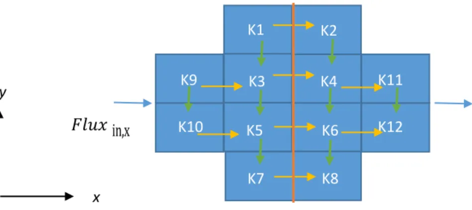
vii value in place of the original ones. The term “equivalent” regards the flux that is kept constant even when the original permeability values are replaced. This method can be considered non-local because the equivalent permeability is influenced by boundary conditions. However, the user has the freedom to use it as a local, because of some available options. Sealed-sides boundary conditions were used in order to force the fluid flows along a principal direction, under a constant gradient of pressure. The flux is forced to flow along a single direction, so it can be globally represented by three systems. Due to this kind of boundary conditions, each system is characterized by a different pressure distribution. In fact, the first step is the three pressure distributions computation. They are necessary in order to calculate the fluxes that are flowing through the three cross-sections. When the fluxes and the pressure distributions are known, they are used to calculate the equivalent permeability first trials. These values replace the original ones in each direction. They cause three new pressure distributions and three different values of fluxes. So, new equivalent permeability values are calculated using the original fluxes because they must be constant. The process starts over and it finishes when the difference between iterative permeability values (in alternative, it is possible to use the fluxes as iterative values) is small enough. The initial idea was modified in order to solve some problems, in particular: convergence and mutual influence among equivalent permeability values. In particular, the final form of the method has the purpose to reach the global homogenization. In other words, it tries to calculate a unique equivalent permeability for all the directions. These modifications have had success because some problems of convergence were solved.
7. Production Well Implementation
Production wells were implemented in the mesh in order to have a comparison between production rates of both systems, the original and the scaled up. It was used the single-layer model, based on the definition of equivalent radius given by Abou-Kassem and Aziz. It is possible to simulate a production well using two approaches: keeping the well flow constant or keeping the sandface pressure constant. In this work, the second option was used because the comparison must be between production rates. The single-layer model was used only for 2D models but it is common in reservoir engineering to neglect the vertical permeability. In other words, it is possible to treat the 3D well model as a 2D, paying attention to some modifications.
viii
8. Results
The results will be shown for two-dimensional and three-dimensional models. The simulation time is a parameter that must be control in order to verify if the upscaling is sufficiently convenient. The results, in terms of computational time, have been satisfactory but it was predictable because of the scale increase. The most important and interesting results regard the difference between well flows. Most of the results, in two and three dimensions, can be considered good (25-50% of error between fluxes) or excellent (0-25% of error between fluxes); if the scale increase is not so marked. When the reservoir size reduction is more marked the model becomes too “approximated” and the well flow errors are no more acceptable. It is important to underline that all the simulations were done with a standard computer, so, it was impossible to simulate huge permeability fields. The results also highlight that most of the times the unsatisfactory well flow errors were obtained when the well-block permeability was too low. It also is an expected result, because it is more difficult to describe and to scale up the fluid flow when the region is characterized by low permeability and the pressure is influenced by the well. Another important aspect regards the heterogeneity. In fact, when the neighbouring blocks of the well block are characterized by highly different permeability values, the difference between flows is higher. Another consideration regards the self-similarity of the model, which is absent. In fact, the permeability probability distribution is not conserved when the original model is scaled. Moreover, after a certain number of scaling application, or in other words when the scaled model is scaled again and again, its permeability probability distribution turns in a Dirac’s Delta distribution.
9. Conclusions and Future Directions
Despite the simple idea on which the method is based, it gave good results. The worst results are obviously correlated with particular aspects that also affect most of the actual upscaling techniques. Due to these “defects” it will be possible to improve this method, trying to develop a better version that is not sensible to high heterogeneous regions or low permeability well-blocks. Moreover, it is possible to extend it for multi-phase and compressible flows.
ix
Riassunto esteso
1. Introduzione
Le tecnologie più avanzate consentono di rendere la rappresentazione di modelli geologici sempre più raffinata e dettagliata. Tali modelli sono rappresentati da maglie discretizzate. Una grande quantità di cellule attive caratterizza i modelli computazionali, purtroppo però non è possibile eseguire le simulazioni in tali condizioni. L’industria petrolifera ha la necessità di usare modelli geologici che siano adatti ai moderni software di simulazione e dunque avere delle stime circa la quantità di olio o gas producibile. Le tecniche di upscaling sono da sempre utilizzate per l’aumento in scala della maglia geologica, consentendo quindi rapide simulazioni di pozzi di produzione/iniezione .
2. Proprietà Fondamentali delle Rocce
Il secondo capitolo è importante per capire e distinguere le proprietà additive da quelle non-additive. La porosità e la permeabilità assoluta sono probabilmente le più importanti per comprendere rispettivamente quale sia il quantitativo di olio nel giacimento e quanto sia quello estraibile. La porosità è definita come il rapporto tra la somma del volume di tutti gli spazi vuoti e il volume totale della roccia. Non tutti gli spazi vuoti però sono connessi e questo aspetto merita di essere preso in considerazione in quanto l’olio non vi può fluire. Infatti, è possibile definire la porosità effettiva come il rapporto tra tutti gli spazi vuoti connessi e il volume totale di tutti gli spazi vuoti. La permeabilità assoluta dipende solo dal tipo di roccia. Comunque, è possibile definirla solo quando il flusso è mono-fasico. Quando un flusso multi-fasico è presente all’interno della roccia, si può definire la permeabilità relativa per ogni fase.
𝑘𝑟𝑝 =𝑘𝑝(100%)𝑘𝑝(𝑆𝑝) (I)
Ai fini di questo lavoro sarà presa in considerazione solo la permeabilità assoluta.
x
3. Principali Tecniche di Upscaling
Il terzo capitolo è una breve descrizione delle principali tecniche di upscaling che sono comunemente usate nell’industria petrolifera. Sono largamente usate, anche quando dovrebbero essere utilizzati metodi numerici, a causa della loro semplice implementazione. Le tecniche che usano semplici medie danno soluzioni estate perchè derivano da una trattazione teorica. La prima importante distinzione deve essere fatta tra proprietà additive e non additive. Infatti, questo tipo di tecniche può essere usato per calcolare il valore equivalente di proprietà additive. Contrariamente con quanto accade per le proprietà non additive, che necessiterebbero di metodi numerici per essere “scalate”. Porosità e permeabilità assoluta sono buoni esempi rispettivamente di proprietà additive e non additive. Questa sezione sarà presentata per comparare i risultati ottenuti dal metodo proposto in questo lavoro e i risultati analitici, quando sono state usate particolari distribuzioni di permeabilità. In questo capitolo saranno definite le seguenti medie:
Media Armonica
Media Aritmetica
Media della Potenza
Medie armoniche ed aritmetiche sono usate in casi differenti. Infatti, la loro applicazione dipende dalla direzione principale lungo la quale la permeabilità cambia significativamente. La media della potenza dipende invece da un parametro, che sarà indicato con p, che a sua volta dipende dalla distribuzione di permeabilità. Un aspetto importante, per i fini di questo lavoro, è la possibilità di combinare le medie armoniche ed aritmetiche per ottenere due tecniche “combinate”, che sono chiamate: Armonica-Aritmetica e Aritmetica-Armonica. Così come per le singole medie armoniche ed aritmetiche, anche queste tecniche combinate devono essere applicate in funzione della direzione principale lungo la quale cambia la permeabilità.
4. Equazioni Basiche per Flusso di Fluido
Il quarto capitolo sarà utile per capire quali equazioni sono state usate. La legge di Darcy è una delle equazioni di base di questo lavoro. Essa è una equazione empirica per flussi mono-fasici ma può essere estesa a flussi multi-fase semplicemente introducendo la permeabilità relativa. La legge di Darcy è caratterizata da limiti pratici. Infatti, essa è basata su semplici assunzioni come:
xi
Flusso laminare
Nessuna interazione chimica o cinetica tra il fluido e la roccia
Fluidi omogenei e Newtoniani
Le equazioni di flusso generalizzate che sono state derivate saranno utili al lettore per avere una guida completa del metodo. Tutte le assunzioni e le ipotesi saranno specificate. Queste equazioni sono basate sul principio di conservazione della massa, partendo da un volume di controllo. L’equazione di conservazione della massa, meglio conosciuta come equazione di continuità, è stata derivata per avere una espressione generale del bilancio di massa per una qualsiasi cella con o senza la presenza del pozzo. Questa espressione è stata inizialmente derivata per un flusso generico, ossia nessuna ipotesi è stata fatta riguardo la natura del fluido. Dopodichè, l’ipotesi di fluido incomprimibile e stato stazionario sono state introdotte.
5. Approssimazione con Differeze-Finite
L’equazione di continuità scritta sotto forma di equazione alle derivate parziali è inutile per i nostri fini, è stato necessario un processo di discretizzazione per renderle implementabili. I processi di discretizzazione più utilizzati in ambito petrolifero sono il metodo alle differenze finite (FDM) e il metodo degli elementi finiti (FEM) ed è stato usato il primo. Il flusso di olio prodotto è funzione dello spazio e del tempo. Quindi è stato necessario discretizzare le equazioni alle derivate parziali nello spazio e nel tempo contenute l’equazione di continuità. Entrambe sono state discretizzate usando l’approssimazione in serie di Taylor. Le derivate spaziali del secondo ordine sono state approssimate usando due volte l’approccio alle differenze centrate. Contrariamente alle derivate temporali, che, essendo del primo ordine sono state approssimate usando l’approccio delle differenze all’indietro.
6. Metodo Numerico di Upscaling Proposto
Il metodo qui proposto è di tipo numerico. Così come per tutti i metodi numerici di upscaling che sono stati sviluppati fin’ora, il processo di omogenizazzione gioca un ruolo fondamentale. In altre parole una regione eterogenea in permeabilità è omogenizzata usando un valore equivalente di tale proprietà. Il termine “equivalente” si riferisce alla conservazione del flusso che passa attraverso una sezione trasversale, anche quando i valori di permeabilità
xii
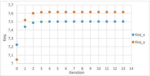
originali vengono sostituiti. Questo metodo può essere considerato un metodo non locale perchè la permeabilità equivalente è influenzata dalle condizioni al contorno; ma allo stesso tempo si da la libertà all’usuario di usarlo come se fosse locale. Le condizioni al contorno utilizzate in questo lavoro forzano il fluido a fluire lungo una direzione, sotto un gradiente di pressione costante arbitrariamente scelto. Il flusso però è forzato ad andare lungo una sola direzione e quindi per rappresentarlo globalmente sono necessari tre sistemi. Dovuto a questo tipo di condizioni al contorno, ogni sistema è caratterizzato da una differente distribuzione di pressione. Infatti il primo passo è il calcolo delle tre distribuzioni di pressione. Esse sono necessarie per calcolare i flussi che stanno fluendo attraverso le tre sezioni trasversali. Quando i flussi e le distribuzioni di pressione sono conosciute, sarà possibile usarle per calcolare i valori di primo tentativo delle permeabilità equivalenti. Questi valori prenderanno il posto dei valori di permeabilità originali lungo ogni direzione. Dovuto a ciò, si avranno tre nuove distribuzioni di pressione che dovranno essere calcolate. Le nuove pressioni daranno come risultato tre nuovi flussi, che saranno diversi dagli originali. Così i nuovi valori di permeabilità equivalente saranno calcolati usando i valori di flusso originali e non quelli iterativi perché il flusso sia costante. Il processo dunque ricomincia e terminerà quando la differenza fra i valori iterativi di permeabilità sarà sufficientemente piccola. L’idea iniziale è stata modificata per risolvere alcuni problemi, in particolare: convergenza e la mutua influenza tra i valori di permeabilità equivalente. In particolare, la forma finale di questo metodo ha come obiettivo la completa omogenizzazione del dominio e quindi tenta di calcolare un unico valore di permeabilità equivalente per tutte le direzioni. Queste modifiche hanno avuto successo perchè hanno risolto gran parte dei problemi di convergenza.
7. Implementazione del Pozzo di Produzione
Il pozzo di produzione è stato implementato al fine di avere una comparazione tra flussi di produzione per entrambi i sistemi (quello originale e quello scalato). È stato usato il modello a singolo strato, basato sulla definizione di raggio equivalente data da Abou-Kassem e Aziz. È possibile simulare un pozzo di produzione usando due approcci: mantenendo il flusso costante o mantenendo la pressione di fondo pozzo costante. Ovviamente è stato scelto il secondo approccio perchè altrimenti la comparazione non avrebbe avuto senso. Il modello a singolo strato è stato usato per il caso di 2D e il 3D usando però i
xiii giusti accorgimenti, ossia trascurando la permeabilità verticale (pratica di uso comune in ingegneria di giacimento).
8. Risultati
I risultati saranno mostrati per i modelli 2D e 3D. Il tempo di simulazione è un parametro importante che deve essere tenuto sotto controllo per verificare se l’upscaling ha avuto l’effetto desirato. I risultati in termini di tempo computazionale sono soddisfacenti anche se ciò era prevedibile, dovuto alla riduzione di risoluzione del modello. I risultati più importanti e interessanti riguardano la differenza tra i flussi. Molti dei risultati, in due e tre dimensioni, possono essere considerati buoni (25-50% di errore tra flussi) o eccellenti (0-25% di errore tra flussi); se l’ aumento in scala non è troppo marcato. Quando l’ aumento di scala è più marcato il modello diventa eccessivamente approssimato e gli errori non sono più accettabili. È importante sottolineare che tutte le simulazioni sono state fatte con un computer standard pertanto è stato impossibile simulare grandi campi di permeabilità. I risultati sottolineano anche che il più delle volte gli errori insoddisfacenti si sono verificati quando il pozzo si trova in una zona di bassa permeabilità. Anche questo è un risultato aspettato, perchè è più difficile descrivere e scalare il flusso di fluido quando la permeabilità è bassa e quando la pressione è influenzata dalla presenza del pozzo. Un altro aspetto importante riguarda il livello di eterogeneità. Infatti, quando i blocchi vicini al pozzo sono caratterizzati da valori di permeabilità altamente differenti, la differenza tra flussi aumenta. Un altro aspetto riguardante il metodo è la sua auto-consistenza, che non è rispettata. Infatti si è visto che applicando l’upscaling sul modello originale la distribuzione di probabilità cambiava. Inoltre applicando il processo di upscaling più volte la distribuzione di probabilità cambiava fino a diventare una distribuzione tipo Delta di Dirac.
9. Conclusioni e Suggerimenti Futuri
A dispetto del fatto che l’idea sulla quale si basa il metodo sia semplice, I risultati ottenuti sono stati buoni. I peggiori risultati sono stati riscontrati per casi particolari che normalmente causano problemi ai processi di upscaling. Dovuto alla presenza di questi difetti sarà possibile migliorare il metodo, tentando di sviluppare una versione migliore che non sia sensibile alle regioni eterogenee o
xiv
di bassa permeabilità. Oltretutto è possibile estendere il metodo per fluidi multi-fase e compressibili.
xv
Contents
Ringraziamenti ... i Sommario ... ii Abstract ... iii Extended Summary ... iv Riassunto esteso ... ix Nomenclature ... xvii List of Figures ... xxList of Tables ... xxii
List of Acronyms ... xxiii
1 Introduction ... 1
2 Fundamental Rock Properties... 3
2.1 Porosity and Effective Porosity ... 4
2.2 Absolute and Relative Permeability ... 5
3 Main Average Upscaling Techniques ... 9
3.1 Heuristic Methods ... 11
3.1.1 Combined Averaging Methods and Directional Averages ... 11
4 Basic Equations for Single-Phase Flow ... 17
4.1 Darcy’s Law ... 17
4.2 Derivation of Generalized Flow Equations in Rectangular Coordinates ... 19
4.3 Incompressible Fluid Flow Equation ... 24
5 Finite – Difference Approximation. ... 27
5.1 Construction of the Grids ... 27
5.2 Spatial Derivatives Approximation ... 30
5.3 Time Derivatives Approximation ... 32
6 Description of the Numerical Upscaling Method ... 35
6.1 Pressure Distribution Calculation ... 36
7 Production Well Implementation ... 57
xvi
8 Results ... 65
8.1 Simulation Time comparison ... 65
8.1.1 Random Permeability Distribution, Simulation Time ... 65
8.1.2 SPE’s Dataset, Simulation Time ... 68
8.2 Production Well Flow Comparison ... 69
8.2.1 Numerical permeability distributions, Well Flow... 70
8.2.2 SPE’s Datasets – Well flow ... 78
8.3 Self-Similarity ... 81
9 Conclusions and Future Directions ... 85
Appendix ... 87
xvii
Nomenclature
𝑉𝑒𝑠 = empty rock volume, [m3] 𝑉𝑡𝑜𝑡 = total rock volume, [m3] 𝜑 = rock porosity𝜑𝑒 = effective rock porosity
𝜑0 = reference effective rock porosity 𝑐𝜑 = porosity compressibility, [kPa-1]
𝑝 = pressure, [kPa]
𝑝0 = reference pressure, [kPa] 𝑆𝑝 = phase saturation
𝑘 = permeability, [mD]
𝑘𝑟𝑝 = relative permeability of the phase p u(𝑥) = filtration velocity, [m3/(day m2)]
∇𝑝 = gradient of pressure, [kPa] 𝐤 = local permeability tensor
𝛽𝑐 = unit conversion factor for the transmissibility coefficient, 86.4 x 10⁻⁶ 𝜌 = density, [kg/m3]
𝜌𝑜= oil density, [kg/m3]
𝜌𝑔= gas density, [kg/m3]
𝑔 = gravity acceleration, 9.81 [m/s2]
𝜇 = fluid viscosity, [Pas] 𝐴 = cross-sectional area, [m2]
𝑞𝑜 = oil flow rate, [m3/day]
xviii
𝜇𝑜 = oil viscosity, [Pas] 𝜇𝑔 = oil viscosity, [Pas]
∆x = difference along x direction, [m] ∆y = difference along y direction, [m] ∆z = difference along z direction, [m] 𝑚𝑖 = mass in, in the control volume, [kg] 𝑚𝑜 = mass out, in the control volume, [kg]
𝑚𝑠 = mass source/sink, in the control volume, [kg] 𝑚𝑎 = mass accumulation, in the control volume, [kg] 𝑤 = mass flow rate, [kg/day]
∆𝑡 = time difference, [day]
𝑞𝑚 = mass production rate, [kg/day]
𝑤𝑥 = mass flow rate in x direction, [kg/day] 𝑤𝑦 = mass flow rate in y direction, [kg/day] 𝑤𝑧 = mass flow rate in z direction, [kg/day]
𝑚𝑥̇ = mass flux vector in x direction, [kg/(day m2)]
𝑚𝑦̇ = mass flux vector in y direction, [kg/(day m2)]
𝑚𝑧̇ = mass flux vector in z direction, [kg/(day m2)]
𝑎𝑐 = volume conversion factor, 5.614583 (for metric unit) 𝑢𝑥 = superficial velocity in x direction, [m3/(day m2)]
𝑢𝑦 = superficial velocity in y direction, [m3/(day m2)]
𝑢𝑧 = superficial velocity in z direction, [m3/(day m2)]
𝐴𝑥 = cross-sectional area normal to x direction [m2]
𝐴𝑦 = cross-sectional area normal to y direction [m2]
xix 𝑉𝑏 = block volume, [m3]
𝐵 = fluid volume factor, [m3/ m3]
𝜌𝑠𝑐 = density at standard conditions, [kg/m3]
𝜌𝑟𝑐 = density at reservoir conditions, [kg/m3]
𝑞𝑠𝑐 = production rate at standard conditions, [std m3/day]
𝑨 = coefficient matrix
𝑘ℎ = horizontal permeability, [mD] 𝑟𝑤 = well radius, [m]
𝐻 = depth of the well, [m] 𝑝𝑤𝑓 = sandface pressure, [kPa] 𝑟𝑒 = external radius, [m] 𝑝𝑒 = external pressure, [kPa] 𝑟𝑒𝑞 = equivalent radius, [m]
𝑓 = fraction of well flow coming from the well-block 𝑟i,j = distance between the block i and the well j, [m] 𝑇𝑖 = interface transmissibility
𝑎𝑗 = distance from the well to its image j, [m]
𝛾wb = multiphase hydrostatic wellbore pressure gradient, [kPa/m] 𝛾c = gravity conversion factor, 10-3
xx
List of Figures
Figure 1.1: Example of upscaling on a porosity field. The fine model (on the left) and the scaled up (on the right) using the harmonic average technique. ... 1 Figure 2.1: A typical hydrocarbons deposit representation. [9] ... 3 Figure 2.2: Example of Relative permeability values in function of Water Saturation. [13] ... 6 Figure 3.1: Example of cells connected in series ... 12 Figure 3.2: Example of cells connected in parallel ... 13 Figure 3.3: Example of Harmonic-Arithmetic technique applied. Step 1 graphically represents the harmonic average applied. Step 2 is the final step, when the arithmetic average is apllied. . 14 Figure 3.4: Example of Arithmetic-Harmonic technique applied. Step 1 graphically represents the Arithmetic average applied. Step 2 is the final step, when the Harmonic average is apllied. 14 Figure 3.5: Example of sealed-sides boundary condition applied on a fine scale model subjected to a constant pressure drop. [12] ... 16 Figure 4.1: Example of control Volume, Basic Reservoir Simulation, Ertekin, King and Abou - Kassem. [19] ... 20 Figure 5.1: Examples of block-centered grid (on the left) and point-distributed grid (on the right). [25] ... 28 Figure 5.2: Example of grid notation. [24] ... 29 Figure 6.1: Example of porous medium through by a fluid along x-axis. ... 36 Figure 6.2: Graphical representation of internal blocks in two dimensions. They are useful in order to describe the mass conservation equations. ... 37 Figure 6.3: Example of mass balance for an external block at the entrance. ... 38 Figure 6.4: Example of coefficient matrix for problems in two dimensions. ... 40 Figure 6.5: Portion of a porous medium in two dimensions... 41 Figure 6.6: Homogenized porous medium on the central region, along x. ... 42 Figure 6.7: Homogenized porous medium along y-direction. ... 43 Figure 6.8: Here an illustration of how represents homogenized permeability grids. ... 46 Figure 6.9: Example of mass balance useful to fine the pressure distribution during the
homogenization process. ... 47 Figure 6.10: Example of convergence using the first version of the method. ... 49 Figure 6.11: Example of convergence using the last version of the method. ... 51 Figure 6.12: Convergence of equivalent permeability values in three dimensions. ... 51 Figure 6.13: Stratified two-dimensional matrix. ... 53 Figure 6.14: Domain taken into account for the test. ... 53 Figure 6.15: Graphical representation of results. On the left, Keq,y; on the right Keq,x. ... 54 Figure 6.16: Example of chessboard matrix. ... 55 Figure 6.17: Graphical representation of results from the chessboard test. ... 55 Figure 7.1: Example of centered well-block (on the left) and off-center well-block (on the right). ... 59 Figure 7.2: Example of off-center well [26] ... 60 Figure 8.1: Graphic Iteration vs Resolution. ... 67
xxi Figure 8.2: Results of simulation time and number of iterations, for a three-dimensional matrix, generated by uniform numerical distribution. ... 67 Figure 8.3: Well flow error in function of fine model’s absolute permeability ... 72 Figure 8.4: Pressure Distributions of Fine and Coarse Model, first test ... 72 Figure 8.5: Error of well flows in function of well-block permeability ... 77 Figure 8.6: Representation of SPE dataset 1 (on the right) and SPE dataset 2 (on the left) ... 79 Figure 8.7: Example of square distribution function ... 81 Figure 8.8: Example of cumulative distribution functions. The green line regards the fine model, while the red and the black ones regard the coarse matrices. ... 82 Figure 8.9: Coarse model's permeability probability distribution functions. ... 82 Figure 8.10: Cumulative distribution functions, turning into a Dirac’s Delta distribution. ... 83
xxii
List of Tables
Table 7.1: Table of Geometric Transmissibilities factors for rectangular geometries [26] ... 62 Table 8.1: Results of simulation time and number of iterations for a two-dimensional matrix generated by uniform numerical distribution. ... 66 Table 8.2: Results of simulation time and iteration number, for a two - dimensional matrix, generated by SPE dataset 1. ... 68 Table 8.3: Results of simulation time and iteration number, for a two - dimensional matrix, generated by SPE dataset 2. ... 69 Table 8.4: Results of production well flows, using a Rectangular Permeability Distribution. .... 70 Table 8.5: Results of production well flows, using a Rectangular Permeability Distribution. .... 71 Table 8.6: Results of production well flows, using a Lognormal Permeability Distribution. ... 73 Table 8.7: Results of production well flows, using a Lognormal Permeability Distribution. ... 73 Table 8.8: Results of production well flows, using a Normal Permeability Distribution,
resolution 2x2. ... 74 Table 8.9: Results of production well flows, using a Normal Permeability Distribution,
resolution 4x4. ... 74 Table 8.10: Results of production well flows for a Rectangular Permeability Distribution, resolution 2x2. ... 75 Table 8.11: Results of well flow for a Rectangular Permeability Distribution, resolution 4x4. .. 75 Table 8.12: Results of well flows for a Log-normal Permeability Distribution, resolution 2x2. 76 Table 8.13: Results of well flows for a Normal Permeability Distribution, resolution 2x2. ... 76 Table 8.14: Results of production well flows, using the SPE's dataset number 1. ... 78 Table 8.15: Results of production well flows, using the SPE's dataset number 2. ... 78 Table 8.16: Results of production well flows, using the SPE's dataset number 2. ... 79 Table 8.17: Well flow results obtained by SPE’s dataset 2 in three dimensions. ... 80
xxiii
List of Acronyms
FDM Finite-Difference Method FEM Finite-Element Method
SPE Society of Petroleum Engineers PDE Partial Differential Equation EOS Equation Of State
1 Introduction
Reservoir simulations are based on conventional and unconventional techniques but both should need a large number of data in order to better describe reservoir properties. [1]
Through advanced instruments, methods and measurements, it is possible to reach a really good knowledge about hydrocarbons deposits and to make accurate three-dimensional geological models. Nowadays, geological models may consist of 10 million active grid blocks, depending on the deposit’s size. [2] Fluid flow simulations in complicated geological model would be impossible to run. Asking a software to elaborate such a great amount of information requires long time and it results, most of the times, in exceeding the practical limits. [3] Actually, reservoir engineers use coarse models from realistic geological ones and apply on them upscaling techniques. Scaled models are made up of a significantly lower number of active grid cells; in this way it is possible to run fluid flow simulations with a reasonable time consumption. [3]
Scaling up a fine geological model is always a fundamental and critical step in reservoir simulation processes. Basically, it is a process which determines the effective property value of a heterogeneous model and it is represented by a correspondent homogeneous model. [4] In other words, it is essentially an averaging procedure where the static and dynamic characteristics of the fine scale model are approximated by those of the coarse one. Figure (1.1) shows an example of averaging procedure on porosity, it was used the harmonic average:
Figure 1.1: Example of upscaling on a porosity field. The fine model (on the left) and the scaled up (on the right) using the harmonic average technique.
This explains why upscaling techniques are nowadays so important and they cannot be avoided. 0 5 10 15 20 25 0 2 4 6 8 10 12 14 16 18 20 0 2 4 6 8 10 12 1 2 3 4 5 6 7 8 9 10
Chapter 1
_______________________________________________________
2
Obviously, change in scale processes are not painless. In fact, replacing a more detailed model with an approximated one, implies the loss several information. The direct consequence is a lower quality prediction of flow rates and pressure distributions. [5]
For additive properties it is easy to achieve a really good approximation of the original fine grid. [6] Volumetric (or additive) properties, such as porosity and saturation, don’t need particular scaling technique. [7] Their “upscaled” representation is given by simple averaging methods, in other words they are obtained applying analytical solutions. [7] However, when dealing with non-additive properties, it is not always possible to approximate effective values by simply using weighted arithmetic average techniques. [8] In fact, in this case, it is necessary to take into account different aspects and the problem gets complicated. A good example is the calculation of absolute permeability [8]. This work is composed of an introductive part, made up of a brief introduction about fundamental rock properties such as porosity and permeability, two important examples of, respectively, additive and non-additive properties.
The second part is about the main average techniques of upscaling for absolute permeability. This part is useful to better understand what kind of tools will be used in this work and why. The third part is the introduction of all the physics concepts, laws, hypothesis and equations on which this work is based. It is advisable for the reader to pay attention to chapters 4, 5 and 7. In particular, chapter 4 illustrates the fluid flow equations on which this numerical method is based. In order to make them useful for the purposes of this work, it was necessary to discretize them through a common discretization process, which is shown in chapter 5. So, chapter 6 is the “heart” of this work. In fact, it will explained how the numerical technique was implemented. All the steps that have contributed to its final form will be shown in chronological order, trying to be as detailed as possible. In chapter 7 will be shown how a production well was implemented in both fine and coarse model. The last part of this work is about the results analysis and conclusions, including advices for future improvements about this method.
2 Fundamental Rock Properties
Hydrocarbons are always situated in deposits. Economically exploitable deposits are composed of two parts: the reservoir and the trap, but only the reservoir has the characteristic of being porous and permeable. [9] Figure (2.1) illustrates how is composed a hydrocarbon deposit. The trap is the upper limit and it is made of a distribution of rocks which holds hydrocarbons inside the reservoir, till it is drilled or broken because of natural movements [9].
Figure 2.1: A typical hydrocarbons deposit representation. [9]
Reservoirs are really complicated systems, characterized by a set of physical parameters, such as porosity, permeability, pressure, temperature, density and the phases which characterize each fluid present in the porous medium. Phases can be gaseous, liquid or solid [9].
For the purpose of this work the most important parameters are porosity and permeability. They are independent of the fluid content, provided that the rock and fluid are nonreactive. In this paragraph porosity and permeability of rocks
Chapter 2
_______________________________________________________
4
will be introduced, together with two fundamentals concepts, namely additive and non-additive properties.
2.1 Porosity and Effective Porosity
Porosity is determined by all the pores, empty spaces and fractures of the rock. It is quantified simply by using a volumetric percentage of empty volumes (Ves) over total volume of the rock (Vtot) [10]:
𝜑 = 𝑉𝑒𝑠
𝑉𝑡𝑜𝑡 (2.1)
Because of its definition porosity is an additive and dimensionless property of the rock. A distinction between total porosity and effective porosity needs to be done. The former, which is defined above, takes into account every single empty space.
Unfortunately, not all the empty spaces are interconnected, therefore hydrocarbons can’t flow through them. Others empty spaces are surrounded by connate water which doesn’t allow hydrocarbons movements. So, effective porosity is defined as the total volume where fluids can flowing (Vees) over the total volume of the rock [10].
𝜑𝑒 =𝑉𝑒𝑒𝑠𝑉𝑡𝑜𝑡 (2.2)
From now on, every time porosity will be mentioned, it will refer to effective porosity. In this sense, porosity is considered a measure of the reservoir capacity for storing fluids.
Porosity varies with depth and horizontal distance and it depends on the nature of the rock. It is influenced by the sedimentation environment as in the space (horizontal variations) as in time (vertical variations). [11]
Because of the rock compressibility, porosity also depends on the pressure, which is usually assumed to be constant. However an expression of porosity in function of pore pressure is given by [11]:
𝜑 = 𝜑0 [1 + 𝑐𝜑(𝑝 − 𝑝0)] (2.3)
Where p0 and 𝜑0are the reference values, in particular p0 is the reference pressure when the porosity is 𝜑0. The reference pressure can be the atmospheric
Fundamental Rock Properties
_______________________________________________________
5 pressure or the initial reservoir pressure at the time t=0. Moreover, 𝑐𝜑 it is the porosity compressibility. [11]
The relation written above expresses the proportionality between porosity and pressure. Apparently it looks a nonsense, but the pressure that is in equation (2.3) regards the pore pressure. So, because of the rock compressibility, when the internal pore pressure increases, the pore expands. [11]
Porosity is evaluated in laboratory, using some rock samples and a porosimeter or others methods, such as neutron-log and formations density, which are subsoil methods. [10]
However, a generic rock property often vary in space, sometimes from a point to another one or from a region to another region. If the property never changes in space, then the rock is defined as homogeneous for that specific property. In the most real cases this situation is never verified, in other words almost all the rocks are heterogeneous. [10]
In particular, reservoir rocks were born because of a long geological process. Nevertheless, sometimes is possible to approximate a heterogeneous region with a homogeneous one, if the variation of the property in space is not statistically important. [11] This kind of approximation helps reservoir engineers to solve problems otherwise intractable [11].
2.2 Absolute and Relative Permeability
Absolute permeability is the most important property for this work, because in single-phase flow it is the most important property to scale up. [12] Absolute permeability allows fluids to flow through the rock, without a physical change of it. [9] If porosity is an interesting parameter for understanding the potential amount of hydrocarbons in a reservoir, permeability is fundamental to understand the potential amount of extractable oil. [11]
It is important to distinguish between absolute permeability and relative permeability. The former is independent of the fluid’s nature and it depends on the rock. [9] It is possible to talk about absolute permeability when the fluid flow is single-phase, otherwise it is necessary to specify the relative permeability. Darcy’s law is based on the assumption of single-phase flow but, in a real situation, all the three phases are present and each one obstacles the movements of the others. [8] This fact it is taken into account by relative permeability that characterize each phase.
Chapter 2
_______________________________________________________
6
It is defined as the effective permeability (expressed in Darcy) for a given saturation of the phase (Sp), over the permeability for a phase saturation of 100% [10].
𝑘𝑟𝑝 =𝑘𝑝(100%)𝑘𝑝(𝑆𝑝) (2.4)
Fluid saturation is simply expressed by the volume of rock filled (𝑉𝑓) by a single phase over the total empty volume (𝑉𝑡). [8]
𝑆𝑝 = 𝑉𝑓𝑉𝑡 (2.5)
Saturation is a dimensionless magnitude, as it is shown on equation (2.5) and it can varies within 0 and 1.
So, relative permeability values, which are dimensionless, are strictly correlated to fluid saturations. For example, when the oil saturation is higher than water saturation, its relative permeability is higher than water relative permeability. [10] An example is shown in figure (2.2):
Figure 2.2: Example of Relative permeability values in function of Water Saturation. [13]
Statistically, to high porosity values correspond high permeability values, in fact a theoretical relationship exists between these two properties. However, for many reasons, points with similar or equal porosity may show significant
Fundamental Rock Properties
_______________________________________________________
7 differences in permeability [10]. In many practical problems, local absolute permeability, it can be represented by three values: kx , ky and kz . [9]
Permeability is not an additive property, unlike porosity. It depends on several factors that are not necessary correlated [10]. This consideration is really important for this work, because it means that simple averaging methods are not always a good approximation of effective (or equivalent) permeability.
3 Main Average Upscaling Techniques
Many upscaling techniques for permeability were, and will be developed using different approaches. From simple statistical averages to advanced numerical methods, the upscaling’s history is still in evolution and it is connected with the necessity of higher quality predictions.
Each upscaling technique is based on homogenization process. This kind of process is essential for the calculation of equivalent permeability. In this chapter will be illustrated different processes for homogenization.
First of all, a distinction should be made among three fundamental concepts concern absolute permeability: equivalent, effective and block permeability. They have different meanings, depending on boundary conditions and heterogeneity level:
Equivalent permeability (Keq-tensor).
The term equivalent indicates a constant permeability tensor that has to represent a heterogeneous medium [14]. Two different approaches are usable in order to calculate the equivalent permeability tensor. The former consists in keeping the flow at the boundaries constant, namely it has to be the same when it flows through the heterogeneous and the homogenized medium. The latter is based on the energy dissipation by the viscous forces in both mediums. Even if these two approaches look different, they are equivalent in case of periodic boundary conditions. However, the perfect equivalence between the real and the fictitious model is impossible to reach [14].
Effective permeability (Kef-tensor).
Effective permeability is the term used for porous mediums that are statistically homogeneous on large scale. In other words, the scale over which the averaged permeability is defined must be larger than the heterogeneity scale within the porous medium [15]. It is an intrinsic property because it does not depends on the macroscopic boundary conditions. Effective permeability has been studied by two different methods, namely stochastic and homogeneous-equation approach [14].
Chapter 3
_______________________________________________________
10
In the first case the permeability field is represented by a random function. Whereas, in the second case the porous medium is supposed to be spatially periodic [14].
Most of the times, reservoirs cannot be considered homogeneous on large scale and, therefore, the basic conditions to calculate effective permeability are not satisfied [14].
Homogenized permeability (or block – permeability, Kb).
Homogenized permeability is the equivalent permeability of a finite-volume block [14]. The concept of statistical homogeneity is not used, unlike the previous definitions. In facts, the block – permeability can be calculated if the block volume is small enough [14]. So, irrespectively of the block being strongly or weakly heterogeneous, the homogenized permeability can be calculated as: [14] 1 𝑉 ∫ u(𝑥)𝑑𝑉 = −𝑲𝑏𝑉 ( 1 𝑉 ∫ ∇𝑝𝑑𝑉 𝑉 ) (3.1)
Where V is the volume of the block (expressed in cm3) and u is the filtration
velocity (by the Darcy’s law, expressed in m/s) and ∇𝑝 is the gradient of pressure (expressed in kPa). Block – permeability is not unique because it depends on the boundary conditions and then it is not an intrinsic property of the porous medium [14].
It is important to understand what the difference among them is because from now on the equivalent grid-block permeability will be the protagonist of this work but, for simplicity, it will be called equivalent permeability.
Upscaling methods can be divided into three principal groups: heuristic, deterministic and stochastic. Deterministic methods imply that the geological model is perfectly known. Different is for stochastic methods, for which, in a first stage, an approximated model has to be considered as a starting point and only then probabilistic techniques are applied on it [14].
Heuristic methods propose formulas to compute equivalent permeability, based on empirical rules [14].
Analytical solutions are obtained from theoretical approaches and they are considered exact solutions. Whereas, numerical solution are often based on approximated approaches, such as discretization of space and time. Due to that, they represent just approximated solutions. However, most of the real cases are
Main Average Upscaling Techniques
_______________________________________________________
11 so complicated that it is impossible to apply analytical formulas, that’s why numerical methods are more important nowadays [14].
In particular, when absolute permeability must be scaled up, there is no applicable analytical solution.
Upscaling methods can be further classified in local and no-local approaches. The formers do not consider the influence of boundary conditions, namely pressure and blocks around the core. As a consequence, the block – permeability is an intrinsic property. It is known from the electrical conductance analogy that arithmetic and harmonic average can be used for mono-dimensional cases [16]. So, local methods are considered a sort of natural extension of the mono-dimensional results and the block-permeability is a function of the core permeability values. Non-local techniques depend on the boundary conditions that influence the flow within the block [16].
The method developed in this work has a dual nature: the user can choose the number of surrounding blocks that must be considered. From now on the number of surrounding blocks will be synthetically called “rings”. The rings around the core, which is the domain subjected to homogenization, are useful to avoid an excessive influence due to the boundary conditions.
Concluding, heuristic methods will be briefly explained in the next paragraph because they are part of this work. In particular, some mathematical tools, such as harmonic and arithmetic averages have been used. Moreover, when the method was tested using particular permeability distributions, they played a fundamental role in order to give the exact solutions of the problem.
3.1 Heuristic Methods
3.1.1 Combined Averaging Methods and Directional Averages
The concept behind these techniques is quite simple: achieving an intermediate value between two theoretical bounds. Averaging techniques are local techniques. Equivalent grid-block permeability, in this case, is an intrinsic property because the boundary conditions do not affect the final result [14].
Chapter 3
_______________________________________________________
12
So, it is possible define the equivalent permeability, 𝑘𝑒, as:
Arithmetic average.
For a dataset k1, ….., kn, it is defined as: [12]
𝑘𝑒 =∑ 𝑘i
𝑛 𝑖=1
𝑛 (3.2)
Harmonic average.
For a dataset k1, ….., kn, it is defined as: [12]
𝑘𝑒 = 𝑛 ∑ 1 𝑘i 𝑛 𝑖=1 (3.3)
These methods are considered as the fastest and intuitively techniques for upscaling. However, those methods could be disadvantageous when a particular rock formation, such as shale rock, is characterized by a permeability value close to zero. In other words, when a non-flow barrier is present in the system. [12]
To this limitation, it has to be added that these methods can only solve 1-D problems in order to determine the effective permeability. So, for how fast and easy they are, it is difficult to apply them on real cases. Most of the reservoir can be considered as vertically homogeneous. It is due to the geological process for which the reservoir was created. Therefore, the main changes of permeability occur horizontally. Averaging methods can be combined together to calculate, for some particular cases, effective permeability. However, they deserve to be described because they will be useful later. Effective permeability can be calculated if permeability is described by a random numeric distribution or if it has a periodic behaviour as a function of space. Depending on the flow direction, effective permeability can be obtained using arithmetic, harmonic or geometric average. For example, for 1-D flow, global effective permeability for a group of cells connected in series, as figure (3.1) shows, can be determined exactly through the harmonic average [16].
Main Average Upscaling Techniques
_______________________________________________________
13 In other words, when the flow is parallel to the main permeability changes, it is possible to use the harmonic average. While, for a plane made up of a single layer of cells crossed by flow perpendicular to the main permeability changes, as figure (3.2) shows, effective permeability can be obtained by using the arithmetic average technique.
Due to that, the arithmetic average (as described in equation (3.4)) is considered the upper bound of the effective permeability. On the other hand, the harmonic average is considered to be the lower bound of the effective permeability. [12] Whereas, geometric average is used when there is no apparent preference for vertical or horizontal flow. [16]
Harmonic and arithmetic techniques can be combined together in order to obtain the so called combined averaging homogenization methods of permeability. Arithmetic-Harmonic and Harmonic-Arithmetic method are also called directional mean methods. [17]
The order of application is important and it depends on the main permeability changes direction.
Harmonic-Arithmetic.
If the permeability main change is parallel to the flow, the harmonic average is applied first, as it is shown in figure (3.3) step 1.
Chapter 3
_______________________________________________________
14
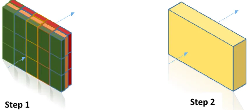
In this way the homogenized columns are connected in parallel, namely the permeability main change is now perpendicular to the flow. So, the arithmetic average is now applicable among homogenized columns, as it is illustrate in figure (3.3) in step 2, obtaining the final, scaled up porous medium. [18]
Arithmetic-Harmonic.
When the fluid flow is perpendicular to the permeability main change direction, then the arithmetic average is used first, giving homogenized plans as it is shown in step 1 of figure (3.4). Now, the permeability main change direction is parallel to the flow and the harmonic average has to be used to calculate the effective permeability of the entire block. The step 2 gives a homogenized domain, illustrate in figure (3.4). [18]
Step 1 Step 2
Figure 3.4: Example of Arithmetic-Harmonic technique applied. Step 1 graphically represents the Arithmetic average applied. Step 2 is the final
step, when the Harmonic average is apllied.
Step 1 Step 2
Figure 3.3: Example of Harmonic-Arithmetic technique applied. Step 1 graphically represents the harmonic average applied. Step 2 is the final
Main Average Upscaling Techniques
_______________________________________________________
15 Sometimes it is possible to substitute the arithmetic or the harmonic average with the geometric one, depending on the permeability main changes direction. Power average. It is defined as: [12] 𝑘𝑒 = √∑ 𝑘𝑖 𝑝 𝑛 𝑖 𝑛 𝑝 (3.4)
It is simply the generalization of all the exponential methods that have been already shown. The power average requires the knowledge of p, which is called power factor. It should be in the range of between -1 and 1. The possible cases are resumed below: [12]
If p = -1, the power average is equivalent to the harmonic average
When p is approximately 0.57 it is the best approximation for horizontal flow in shale-sand environments.
When p = 1, it coincides with the arithmetic average
For p = 0.12, it is the best characterization of vertical flows.
To conclude this section can be interesting to introduce one of the most used numerical approach. Most of the numerical methods require to solve the flow equation at the fine scale for portions of reservoir. This kind of approach requires computational time. The diagonal tensor is based on periodic boundary conditions and nowadays is one of the most approach used. [12]
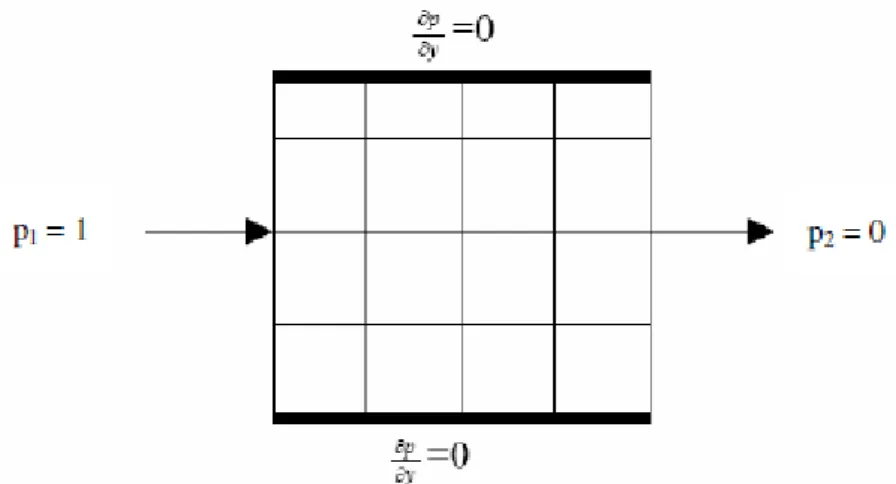
Darcy’s Law equation is solved in order to guarantee the mass conservation, or in other words, a constant flow at the borders. Boundary conditions and pressure drop are applied in order to determine the effective properties, such as figure (3.5) shows: [12]
Chapter 3
_______________________________________________________
16
Most of the times numerical methods are iterative. The one that is proposed in this work follows this kind of approach, but it will be better explained in the next chapters. However, it is possible to anticipate that the sealed-sides boundary conditions and the pressure drop as it is shown in figure (3.5), were used in this work.
Figure 3.5: Example of sealed-sides boundary condition applied on a fine scale model subjected to a constant pressure drop. [12]
4 Basic Equations for Single-Phase Flow
This work is based on simple equations that describe single-phase fluid flows inside a porous medium. All the mathematical equations derive from physical processes and considerations that concern reservoirs. Because of that, they will be initially expressed in form of Partial-Differential Equations (PDEs) that include the dynamic relationships among the fluid flow, mechanical and physical properties of the porous medium and, obviously, flow conditions of the system.
4.1 Darcy’s Law
The purpose of this paragraph is to introduce clearly the Darcy’s Law for single-phase flow in three-dimension. The most famous law used in reservoir simulation is Darcy’s law, obviously for fluid flowing in a porous medium. Darcy’s law is an empirical relationship between fluid flow rate and pressure gradient (or hydraulic gradient). Its mathematical expression is [13]:
𝑞 = −𝛽𝑐𝐤𝜇∗ (𝛻𝑃⃗⃗⃗⃗⃗ − 𝜌𝑔) ∗ 𝐴 (4.1)
Where 𝛽𝑐 it is the unit conversion factor for the transmissibility coefficient (its value is 86.4 x 10⁻⁶, to convert magnitudes of the metric system), 𝐤 is the absolute rock permeability tensor, 𝜇 is the fluid viscosity (expressed in centipoise or in Pas), 𝛻𝑃⃗⃗⃗⃗⃗ is the gradient of pressure, 𝜌𝑔 is the gravitational term (𝜌 is expressed in kg/m3 and 𝑔 in m/s2) and 𝐴 is the cross-sectional area
(expressed in m2). [13]
Equation (4.1) is the basis for any understanding and prediction of flow. Permeability appears in Darcy’s law as local permeability tensor, mathematically represented by 𝐤, as shown here [15]:
𝐤 = [𝑘𝑥𝑥 𝑘𝑥𝑦 𝑘𝑥𝑧𝑘𝑦𝑥 𝑘𝑦𝑦 𝑘𝑦𝑧 𝑘𝑧𝑥 𝑘𝑧𝑦 𝑘𝑧𝑧
![Figure 2.1: A typical hydrocarbons deposit representation. [9]](https://thumb-eu.123doks.com/thumbv2/123dokorg/7500657.104470/29.892.190.750.476.809/figure-a-typical-hydrocarbons-deposit-representation.webp)
![Figure 2.2: Example of Relative permeability values in function of Water Saturation. [13]](https://thumb-eu.123doks.com/thumbv2/123dokorg/7500657.104470/32.892.238.644.640.948/figure-example-relative-permeability-values-function-water-saturation.webp)