Comparison of MLP, RNN and CNN machine learning algorithms for damage detection exploiting ultrasonic Lamb waves

(1)

School of Industrial and Information Engineering Department of Mechanical Engineering

Master of Science in Mechanical Engineering

Comparison of MLP, RNN and CNN Machine

Learning algorithms for damage detection

exploiting ultrasonic Lamb waves

Supervisor:

Prof. Claudio Sbarufatti Co-supervisor:

Dr. Stefano Mariani

Author: Matteo Urbani

(2)

(3)

(4)

(5)

Abstract

A large number of different techniques are used for structural health monitoring purposes. In this thesis the physical phenomenon of Lamb waves is exploited, this being elastic waves that propagate in solid materials of small thickness (i.e. plates). Specifically, a 500x500x5 mm steel plate was simulated using a Finite Element software, within which Lamb waves were excited by means of a simulated piezoelectric sensor placed in the center of the plate. A second simulated piezoelectric sensor was positioned at various locations of the plate and was used as receiver. The signal acquired by the second sensor comprises both the direct arrival of the waves transmitted by the actuator and the reflections of the latter from the edges of the plate and from any damage introduced inside the plate itself. Reading and interpretation of the acquired signals was performed via three different sets of Machine Learning (ML) algorithms: multilayer perceptron (MLP), Long Short-Term Memory (LSTM) and WaveNet (an algorithm based on deep convolutional neural networks recently developed for acoustic applications).

The use of a numerical model was essential to generate the high number of examples necessary to train the tested algorithms. The dataset on which the analyses were performed contains signals acquired by the simulated receiver placed in three different locations of the plate, in both undamaged (baseline case) and damaged conditions (obtained by adding a through-thickness defect at 100 different positions), both for temperatures varying from 20°C to 69°C at steps of 1°C (50 temperatures). The instrumentation noise effect have been included into the signals with various levels of intensity, to make them more realistic. The temperature effect was partially compensated using the Baseline Signal Stretch (BSS) technique, the only signal pre-processing tool required for the methodology discussed in this thesis.

The main task of this work was to determine the hyperparameters for each type of ML algorithm that would give the best defect detection performance. WaveNet was proven to be the best algorithm for the task when considering computation speed, ease in hyperparameters tuning and accuracy of defect detection, which reached 100% in a number of cases.

WaveNet was then tested in two other contexts. The first concerned the robustness of the algorithm in evaluating signals acquired at temperatures outside the range used for its training: the measured performance was largely satisfactory, with 100% detection accuracy reported for signals acquired up to 30°C beyond the training range. The second aimed to validate its performance when applied to a real dataset. The experimental set was acquired under a similar configuration to that used in the numerical simulations, although the plate was made of composite material and the excitation frequency was significantly lower. However, in some cases the algorithm was able to completely discern the signals with defect from those without defects, hence suggesting a strong adaptation capability that can be exploited in different applications.

(6)

(7)

Sommario

Un gran numero di tecniche differenti viene utilizzato nell’ambito del monitoraggio strutturale. In questa tesi viene sfruttato il fenomeno fisico delle onde di Lamb, onde elastiche che si propagano in materiali solidi di piccolo spessore (i.e. piastre). In particolare, una piastra in acciaio da 500x500x5 mm è stata simulata utilizzando un software agli elementi finiti, all'interno del quale le onde di Lamb sono state eccitate per mezzo di un sensore piezoelettrico simulato posto al centro della piastra. Un secondo sensore piezoelettrico simulato è stato collocato in varie posizioni della piastra e utilizzato come ricevitore. Il segnale acquisito dal secondo sensore comprende l'arrivo diretto delle onde trasmesse dall'attuatore e le loro riflessioni date dai bordi della piastra e da qualsiasi danno introdotto all'interno della piastra stessa. La lettura e l'interpretazione dei segnali acquisiti sono state affidate a tre diversi set di algoritmi di Machine Learning (ML): multilayer perceptron (MLP), Long Short-Term Memory (LSTM) e WaveNet (un algoritmo basato su reti neurali convoluzionali recentemente sviluppato per applicazioni acustiche).

L'uso di un modello numerico è stato essenziale per generare l'alto numero di esempi necessari ad addestrare gli algoritmi testati. Il dataset su cui sono state eseguite le analisi contiene segnali acquisiti dal ricevitore simulato posto in tre diverse posizioni sulla piastra, sia in condizioni non danneggiate (caso base) che in condizioni danneggiate (ottenute con l’aggiunta di un difetto passante collocato in 100 posizioni differenti), entrambe per temperature che variano tra i 20°C ed i 69°C con step di 1°C (50 temperature). L'effetto del rumore della strumentazione è stato incluso nei segnali con vari livelli di intensità, per renderli più realistici. L'effetto della temperatura è stato parzialmente compensato utilizzando la tecnica Baseline Signal Stretch (BSS), unico strumento di pre-processing dei segnali richiesto per la metodologia discussa in questa tesi.

Il compito principale di questo lavoro è stato determinare gli iperparametri per ogni tipo di algoritmo di ML che avrebbero dato le migliori prestazioni nel rilevamento dei difetti. È stato dimostrato come WaveNet sia l'algoritmo migliore per tale scopo considerando velocità di calcolo, facilità nella messa a punto degli iperparametri e accuratezza nel rilevamento dei difetti, la quale ha raggiunto il 100% in diversi casi.

WaveNet è stato quindi testato in altri due contesti. Il primo riguardava la robustezza dell'algoritmo nella valutazione di segnali acquisiti a temperature al di fuori dell'intervallo utilizzato per il suo allenamento: le prestazioni misurate sono state ampiamente soddisfacenti, con un'accuratezza nel rilevamento del 100% ottenuta per segnali acquisiti fino a 30°C oltre l'intervallo di allenamento. Il secondo mirava a convalidare le sue prestazioni quando applicato ad un set di dati reale. Il set sperimentale è stato acquisito con una configurazione simile a quella utilizzata nelle simulazioni numeriche, sebbene la piastra fosse realizzata in materiale composito e la frequenza di eccitazione fosse significativamente inferiore. Tuttavia, in alcuni casi l'algoritmo è stato in grado di discernere completamente i segnali con difetto da quelli senza difetti, suggerendo quindi una forte capacità di adattamento che può essere sfruttata in diverse applicazioni.

(8)

(9)

Figures

Fig. 1: symmetric (left) and anti-symmetric (right) mode shapes of Lamb waves ... 5

Fig. 2: operations occurring inside a single neuron ... 8

Fig. 3: most common types of activation functions ... 8

Fig. 4: overfitting to the training set can be seen in the cost function of the validation set, which starts to increase after about 100 steps ... 12

Fig. 5: steel plate dimensions and position of the emitter ... 16

Fig. 6: position of defects on the plate... 16

Fig. 7: position of the available receivers on the plate ... 17

Fig. 8: mirroring scheme of the solutions of the FE simulations. Red circles represent the defects for which the solution of the numerical problem has been computed via numerical simulations; green circles represent the defects for which the solution of the numerical problem has been obtained by mirroring those of the symmetric red “parent” defects. The symmetries exploited are the horizontal and vertical dash-dot axes passing by the centre of the plate. Darker circles highlight an example of set of defects for which the numerical solution is equivalent but symmetric. ... 18

Fig. 9: locations of the three receivers used in this study ... 18

Fig. 10: dispersion curves for a steel plate 5mm thick. In the upper plot is represented the phase velocity while in the lower plot is represented the group velocity. Red lines represent Sn modes while blue lines represent A0 modes. The dashed line indicate the chosen excitation frequency (300 kHz) ... 20

Fig. 11: final shape of the excitation signal ... 20

Fig. 12: example of one signal coming from the numerical simulations ... 22

Fig. 13: minimum travel distance of the signal to capture defect information ... 23

Fig. 14: signals captured by the receiver placed in the three chosen locations ... 24

Fig. 15: signals taken at three different temperatures ... 26

Fig. 16: signals taken at three different temperatures after BSS ... 26

Fig. 17: example of noise after it has been filtered in 270-330 kHz bandwidth ... 28

Fig. 18: two macro sets of lines are represented: the first three of the legend represent the maximum absolute values of the defects’ reflections for all the temperatures for three receivers; the last four of the legend represent four times the standard deviation of the four noise levels. Each line is normalised with respect to the maximum absolute value of the pristine signal collected by receiver 1 (about 45 mm from the emitter). ... 28

(12)

Fig. 19: impact of a defect in Lamb waves propagation for noise-less signals; defect nr.79, which produced the largest reflection seen by receiver 2;

pristine and defective signals are taken at the same temperature ... 29 Fig. 20: impact of a defect in Lamb waves propagation for signals with the lowest

noise (SNR 1); defect nr.79, which produced the largest reflection seen by

receiver 2; pristine and defective signals are taken at the same temperature .... 29 Fig. 21: impact of a defect in Lamb waves propagation for signals with the

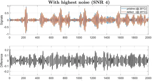
highest noise (SNR 4); defect nr.79, which produced the largest reflection seen by receiver 2; pristine and defective signals are taken at the same

temperature ... 30 Fig. 22: impact of a defect in Lamb waves propagation for noise-less signals;

defect nr.71, which produced the lowest reflection seen by receiver 2;

pristine and defective signals are taken at the same temperature ... 30 Fig. 23: impact of a defect in Lamb waves propagation for signals with the lowest

noise (SNR 1); defect nr.71, which produced the lowest reflection seen by

receiver 2; pristine and defective signals are taken at the same temperature .... 31 Fig. 24: impact of a defect in Lamb waves propagation for signals with the

highest noise (SNR 4); defect nr.71, which produced the lowest reflection seen by receiver 2; pristine and defective signals are taken at the same

temperature ... 31 Fig. 25: impact of a defect in Lamb waves propagation for noise-less signals;

defect nr.79, which produced the largest reflection seen by receiver 2;

pristine and defective signals are taken at temperatures differing of 1°C ... 32 Fig. 26: impact of a defect in Lamb waves propagation for signals with the lowest

noise (SNR 1); defect nr.79, which produced the largest reflection seen by receiver 2; pristine and defective signals are taken at temperatures

differing of 1°C ... 32 Fig. 27: impact of a defect in Lamb waves propagation for signals with the

highest noise (SNR 4); defect nr.79, which produced the largest reflection seen by receiver 2; pristine and defective signals are taken at temperatures differing of 1°C ... 33 Fig. 28: impact of a defect in Lamb waves propagation for noise-less signals;

defect nr.71, which produced the lowest reflection seen by receiver 2;

pristine and defective signals are taken at temperatures differing of 1°C ... 33 Fig. 29: impact of a defect in Lamb waves propagation for signals with the lowest

noise (SNR 1); defect nr.71, which produced the lowest reflection seen by receiver 2; pristine and defective signals are taken at temperatures

differing of 1°C ... 34 Fig. 30: impact of a defect in Lamb waves propagation for signals with the

(13)

seen by receiver 2; pristine and defective signals are taken at temperatures

differing of 1°C ... 34

Fig. 31: division of defects positions in training set (blue), validation set (green) and test set (red). The order of defects’ numbers is the one used in Matlab and Python codes, it does not have any particular meaning ... 36

Fig. 32: division of defects and pristine temperatures in training set (blue), validation set (green) and test set (red) ... 36

Fig. 33: visual intuition of the difference between gradient descent and Adam algorithms ... 41

Fig. 34: mini-batch technique influence on loss function minimisation procedure ... 42

Fig. 35: architecture of MLP Neural Network ... 45

Fig. 36: MLP - accuracy plots: 1 hidden layer ... 47

Fig. 37: MLP - accuracy plots: 2 hidden layers ... 47

Fig. 40: MLP - test accuracy comparison ... 49

Fig. 41: MLP - loss plot: representative case of the trend of training and validation losses along epochs... 49

Fig. 42: concept of regularization effect when neural networks tend to overfit over the training set ... 50

Fig. 43: visual representation of dropout, which randomly sets to zero some neuros ... 51

Fig. 44: MLP - accuracy plots: 1 hidden layer with dropout regularisation ... 51

Fig. 45: MLP - accuracy plots: 2 hidden layers with dropout regularisation ... 52

Fig. 48: MLP - accuracy plots: 1 hidden layer with L2 regularisation ... 53

Fig. 49: MLP - accuracy plots: 2 hidden layers with L2 regularisation ... 54

Fig. 52: MLP - accuracy plots: 1 hidden layer, comparison among different regularisers ... 55

Fig. 53: MLP - accuracy plots: 2 hidden layers, comparison among different regularisers ... 55

Fig. 56: MLP - loss plots: learning case without any regulariser ... 57

Fig. 57: MLP - loss plots: learning case with dropout regulariser (𝑝 = 0.2) ... 57

(14)

Fig. 59: MLP - accuracy plots: 3 hidden layers, second set of trainings ... 59

Fig. 60: MLP - accuracy plots: 4 hidden layers, second set of trainings ... 59

Fig. 61: MLP – test set accuracy plots: 3 and 4 hidden layers, comparison between the cases with neurons distributed in decreasing order (left, first set of training with L2 regulariser) and neurons distributed in increasing-decreasing order (right, second set of training with L2 regulariser) ... 60

Fig. 62: MLP - accuracy plots: 1 hidden layer, final set of runs ... 61

Fig. 63: MLP - accuracy plots: 2 hidden layers, final set of runs ... 61

Fig. 66: PCA transformation – x represents the original reference system, x’ represents the principal reference system ... 63

Fig. 67: PCA - cumulative sum of eigenvalues for different SNR levels, sensor 1 ... 64

Fig. 70: difference between an example and its reconstruction with only the first principal component – noise-less case ... 65

Fig. 71: difference between an example and its reconstruction with only the first principal component – SNR 1 case ... 66

Fig. 72: difference between an example and its reconstruction with only the first principal component – SNR 4 case ... 66

Fig. 73: difference between an example and its reconstruction with the first 200 principal components – noise-less case ... 67

Fig. 74: difference between an example and its reconstruction with the first 200 principal components – SNR 1 case ... 67

Fig. 75: difference between an example and its reconstruction with the first 200 principal components – SNR 1 case ... 68

Fig. 76: difference between an original signal and the same after it has been transformed by PCA ... 68

Fig. 77: MLP - accuracy plots: 1 hidden layer, PCA ... 69

Fig. 78: MLP - accuracy plots: 2 hidden layers, PCA ... 69

Fig. 81: visual representation of the operations computed inside an LSTM cell: rectangles represent a linear combination of its inputs, rhombus represent an operator and the two tanh are activation functions mapping directly inputs to outputs ... 74

Fig. 82: LSTM - accuracy plots: 1 and 2 layers ... 76

Fig. 83: LSTM - loss plot: representative case of the trend of training and validation losses along epochs... 77

(15)

Fig. 85: scheme of WaveNet architecture ... 80

Fig. 86: WaveNet - accuracy plots: dd=4, ks=2 ... 82

Fig. 92: WaveNet - test accuracy plots: comparison for all the hyperparameters used ... 84

Fig. 93: WaveNet - loss plot: representative case of the trend of training and validation losses along epochs... 85

Fig. 94: WaveNet - accuracy plots: final set of runs ... 86

Fig. 95: WaveNet – distribution of the predictions of a model when test set examples are fed as input ... 86

Fig. 96: architectures comparison - test accuracy plots, SNR 1 ... 87

Fig. 100: division of defects and pristine temperatures for extrapolation case: training set (blue), validation set (green) and 3 test sets (yellow, orange and red respectively) ... 94

Fig. 101: accuracy plots for temperature extrapolation test – SNR 1 ... 96

Fig. 105: CFRP plate dimensions and positions of emitter, receiver and defects ... 100

Fig. 106: example of experimental signal ... 100

Fig. 107: impact of defect nr. 1 in Lamb waves propagation for experimental signals; pristine and defective signals are taken at the same temperature ... 101

Fig. 111: impact of defect nr. 1 in Lamb waves propagation for experimental signals; pristine and defective signals are taken at temperatures differing of 1°C ... 103

Fig. 112: impact of defect nr. 2 in Lamb waves propagation for experimental signals; pristine and defective signals are taken at temperatures differing of 1°C ... 103

(16)

Fig. 113: impact of defect nr. 3 in Lamb waves propagation for experimental signals; pristine and defective signals are taken at temperatures differing of 1°C ... 103 Fig. 114: impact of defect nr. 4 in Lamb waves propagation for experimental

signals; pristine and defective signals are taken at temperatures differing of 1°C ... 104 Fig. 115: division of defects and pristine temperatures in training set (blue),

validation set (green) and test set (red) for the experimental dataset ... 105 Fig. 116: WaveNet - accuracy plots with experimental dataset using defect in

position 1 to validate the algorithm ... 107 Fig. 117: WaveNet - accuracy plots with experimental dataset using defect in

(17)

Tables

Tab. 1: locations of the three receivers used in this study ... 19

Tab. 2: phase and group velocities for S0 and A0 modes for an excitation source of 300 kHz ... 20

Tab. 3: material properties for the considered range of temperatures, i.e. from 20°C to 69°C ... 21

Tab. 4: first arrival times computed from dispersion curves data ... 24

Tab. 5: number of defect and pristine examples in every set – unbalanced distribution ... 37

Tab. 6: number of defect and pristine examples in every set – balanced distribution ... 37

Tab. 7: MLP architecture hyperparameters - first set of runs ... 46

Tab. 8: number of neurons for every hidden layer in MLP architecture ... 46

Tab. 9: number of neurons for every hidden layer in MLP architecture: second set of trainings ... 58

Tab. 10: MLP architecture hyperparameters - final set of runs ... 61

Tab. 11: MLP architecture hyperparameters - PCA ... 69

Tab. 12: LSTM architecture hyperparameters - first set of runs... 75

Tab. 13: LSTM architecture hyperparameters - final set of runs ... 78

Tab. 14: WaveNet architecture hyperparameters - first set of runs ... 80

Tab. 15: WaveNet architecture hyperparameters - final set of runs... 85

Tab. 16: architectures comparison – training duration ... 89

Tab. 17: number of defect and pristine examples in every set for extrapolation case – unbalanced distribution ... 94

Tab. 18: number of defect and pristine examples in every set for extrapolation case – balanced distribution ... 95

Tab. 19: position of sensors and defects on the CFRP plate ... 100

Tab. 20: number of defect and pristine examples in every set of the experimental configuration – unbalanced distribution ... 105

Tab. 21: number of defect and pristine examples in every set of the experimental configuration – balanced distribution ... 106

(18)

(19)

Introduction

Every mechanical system is designed based on theoretical and numerical models which cannot account for all the possible environmental conditions or events that might interfere with the system during its life cycle. Years of experiments and tests on the most common components and loading conditions have been made, which allowed a fine tuning of coefficients that can be used to correct theoretical models’ predictions and increase their accuracies. However, relying on the component’s lifetime predicted a priori by a model can be an inconvenient approach: at the end of its predicted life the component is substituted no matter its actual condition; it can be worn enough to negatively affect the performance of the entire system (thus its substitution is correct) as well as still working properly (thus its substitution turns out to be a loss of resources); in the worst case the component can break before the end of its predicted life-cycle causing damages to other components, forced stop of the entire system, supplementary maintenance and, most importantly, safety issues.

An approach to assess the condition of mechanical structures relies on data acquisition from the actual working system and their elaboration. This approach is based on the ability to read and extract important information from sensors in order to understand whether there is the necessity to intervene with corrective actions in the structure, i.e. maintenance procedures. Based on the frequency, a classification of different maintenance approaches can be identified:

 planned (preventive) maintenance: control of components’ health is taken at fixed-time intervals, decided during components and system design stage;

 predictive maintenance: it relies on both theoretical models and measurements (temperature, pressure, chemical composition, vibrations, noise…) which are analysed each time the maintenance is scheduled. The date of the following

(20)

maintenance is decided based on the data acquired, which are used to predict the remaining life of every component;

 condition-based maintenance: maintenance is executed only when one or a set of monitored sensors register unacceptable levels of certain parameters.

When maintenance is required the system must be stopped and completely dismantled in order to assess the actual state of every component. This is a drawback for planned maintenance since it is done regardless of the need of a component to be repaired or substituted. This type of maintenance is suited for small and cheap systems where downtimes are not much relevant and do not lead to economic issues: the smaller and simpler the system, the faster and cheaper the maintenance.

When systems become bigger, more complex and more expensive, it may be worth buying high quality sensors and acquisition systems to have a more accurate control of its status. The initial costs are not negligible but can be justified by a lower maintenance frequency, which means lower downtimes, better usage of resources and economic savings. Predictive maintenance is in fact applied when downtime-related costs are considerable, e.g. Loss of profits during downtime or direct maintenance labour cost.

Condition-based maintenance is the extreme version of predictive maintenance. Initial costs can be even higher due to the need of a larger number of sensors to be installed on the structure; furthermore, sensors and acquisition system bust be run frequently in order to promptly indicate the eventual presence of a malfunctioning. The great advantage of this maintenance technique is that it is able to detect abrupt changes on the health state of the monitored system, that would be impossible for the other two techniques for which the system is monitored only at certain intervals. All these considerations justify condition-based maintenance only in fields where structures are big, complex and subjected to damages related to unpredictable external agents.

Structural Health Monitoring (SHM) is a condition-based monitoring method whose aim is to detect the presence of damages in structures. This is done by acquiring signals from different sensors and extracting useful information about the presence of defects, which affect physical characteristics of the structure. In this thesis Lamb waves are exploited in a SHM framework to assess the presence of a defect in a simulated steel plate. Lamb waves propagate in solid mediums and are reflected either by boundaries of the geometry of the structure or by defects and damages (cracks, holes, corrosion…). These imperfections alter shape and direction of the waves, hopefully allowing to detect presence, location and entity of the damage. Since Lamb waves are extremely complex, it is not straightforward to extrapolate information from them, thus Artificial Intelligence (AI) algorithms can be exploited to develop reliable monitoring systems to be used in real cases.

(21)

Thesis background

Several studies have been reported in literature about the interpretation of Lamb wave signals with Machine Learning algorithms for health monitoring purposes. One of the leading fields is the aeronautical one where the complexity of aircrafts requires high levels of accuracy in interpreting the health state of the structure; the increasing performance of health monitoring techniques is spreading also to high speed trains, railways, pipelines, wind turbines and many others.

Most of the works follow a similar trend, which consists in the following steps:  identification of material and geometry of the structure to be analysed;

 choice of sensors in terms of typology (usually piezoelectric), quantity and position;

 setting of the numerical model used to create the dataset needed to train ML algorithms;

 identification of pre-processing techniques to be used to clean signals or extract particular features;

 build ML algorithms in order to have the required outputs, which usually are detection of a defect and its localisation and damage quantification;

 training of ML algorithms;

 validation of ML algorithms with signals obtained from experimental tests. Structures are usually made from the well-known steel and aluminium materials to the latest more advanced and promising composite materials, mainly reinforced with carbon fibres. The typical structure analysed consists in a simple square plate, which guarantees both ease of production (necessary to experimentally validate the model) and good generalisation of the obtained results. The quantity of sensors used can be high in order to create a grid or a network; in any case they are mainly used in couples of emitter and receiver and different combinations are tested to understand any possible relation between their position in the structure and relatively to the defects.

The stages that mainly differ between Lamb-waves-based SHM studies involve the pre-processing techniques of the signals and the typology of ML algorithms implemented. Signals coming from numerical simulations are lacking stochastic disturbances, thus are usually contaminated with artificial noise (e.g. white noise) at different amplitudes in order to make them closer to reality. Before being fed to the ML algorithms, the dataset can be pre-processed for the following reasons:

 cut the signal to consider only the most significant part: by knowing material characteristics and geometry of the plate it is possible to find the time needed for

(22)

the excitation to reach the sensor (i.e. time of flight, tof), allowing to collect the signal with a certain delay and shorten its length;

 reduce the dimensionality of the signal to account for only the most significant features: for example Principal Component Analysis (PCA) is a technique that allows to transform the dataset of signals and reduce its dimensions without losing the most important information of the signal;

 compensate effects given by change in temperatures: it is a well-known issue affecting the shape of Lamb wave signals. Among all the techniques can be found baseline signal reconstruction, baseline signal stretch (BSS) [1] [2], orthogonal matching pursuit;

 extraction of different features: an example can be transforming the dataset of signals from time domain to frequency domain with a Fourier transformation; in some cases also some error indexes can be extracted from the signals, like the Root Mean Square Error (RMSE) between 2 signals, the difference between peaks, the delay of some waves.

For what concerns the ML algorithms it is quite common the usage of multilayer perceptrons (MLPs), which are the most basic types of neural networks and thus the easiest to implement. Also Support Vector Machines (SVMs) are often used for defect detection: they are supervised-learning algorithms that can be used to distinguish whether an input belongs to one class or the other (only binary classification). It is rarer to find the implementation of Recurrent Neural Networks (RNNs) and only during the very last few years Convolutional Neural Networks (CNNs) started to spread their benefits into Lamb waves interpretation in SHM framework.

The accuracies obtained in detection, localisation and damage quantification may largely vary depending on the choices of materials, measurement setup, pre-processing of signals, architecture of ML algorithm and many other parameters. These kind of monitoring systems can correctly detect, localise and quantify even the entire dataset of signals used in specific cases, which is the reason why ML algorithms are becoming increasingly used to extract important features from Lamb waves. However, AI is a fast growing field nowadays but it is still difficult to deal with its complexity: most of the times it is still preferred to rely on deterministic rearrangements (pre-processing of datasets) rather than feeding signals acquired from sensors directly to ML algorithms, which are more difficult to interpret since they act as black boxes whose internal behaviour is not easily understandable. That is the reason why several (sometime sophisticated) types of pre-processing stages are still implemented before feeding inputs to the ML algorithms. This is only a brief summary of the key points representing the state of the art in health monitoring field exploiting Lamb waves. Several articles can be found in literature regarding these topics; few of these are [3] [4] [5] which furnished helpful ideas to undertake the work made for this thesis.

(23)

In the following two chapters a brief introduction to Lamb waves and ML algorithms is reported.

Lamb waves

Lamb waves are elastic waves propagating in thin plates. They are formed by the displacement of particles in the material with energy moving radially along the plate with respect to the excitation point and normal to the plate’s surfaces. In the ideal case of an infinite medium these waves are composed by only two modes: symmetric (S0,

longitudinal or pressure waves, Fig. 1-left) and antisymmetric (A0, transverse or shear

waves, Fig. 1-right). When plates are considered the medium is confined between two surfaces and infinite pairs of modes (symmetric and antisymmetric) arise; these propagate in longitudinal and transverse directions, denoted with Sn and An respectively, being n

the number of the mode pair [6]. Below a certain frequency only fundamental modes S0

and A0 are present; when it comes to higher frequencies other modes sums up and create

a wave with increasing complexity. In order to limit the complexity, the excitation signal is commonly generated at a frequency low enough to excite only the fundamental modes. Nonetheless, presence of defects may also distribute wave’s energy towards higher frequencies allowing the propagation of other modes [4], raising the complexity of the problem.

Every single mode is characterised by two velocities: group velocity and phase velocity, which are respectively the speed at which the envelope and the phase of the waves propagate. The former can be used to identify the time needed for the wave to travel at a certain distance, so can be used to properly set the acquisition time of the signal. Both velocities turn out to be dispersive, which means that they depend on the frequency of the excitations: it is unfeasible to generate an excitation signal with a bandwidth narrow enough to excite only one frequency, so the generated wave will not be able to maintain the same shape as it propagates. This adds another level of complexity to the signal.

In SHM framework these waves can be used to detect the presence of a defect: when the wave encounters a local change in material properties or geometry of the plate (e.g. stiffness reduction due to a void left by a crack) a certain amount of energy is scattered

(24)

and released radially from it. This generates another wave propagating in all directions, which sums up to the original wave. The difference in wave propagation can be detected by a sensor and can give useful information about the presence of a defect and possibly also about its location and severity.

The reflection of the waves depend on how much they are sensitive to changes in the plates: neglecting any dissipation of the energy, at the boundaries of the plate the waves are completely reflected back symmetrically with respect to the normal of the boundary; when instead the wave encounters a defect it is not completely reflected: depending on its dimension, a part of the energy of the wave will continue to propagate past the defect, while the other portion will be radially scattered from it. The amount of scattering will greatly depend on the relative dimensions of the wavelength and size of the defect and it becomes very low when the former is much larger than the latter.

Machine Learning

Machine Learning (ML) is the name used to identify algorithms that are capable of accomplishing a large variety of tasks by learning through experience. It is like a software that improves itself learning from its own mistakes, which is why it belongs to AI framework. These types of algorithms are broadening their fields of application during the last decades thanks to the continuous improvement of computational power, which is one of the key factors that allows AI to be actually applied in industries. ML algorithms are already applied for different purposes, like Natural Language Processing (NLP, e.g. Alexa from Amazon or Siri from Apple) or computer vision (e.g. self-driving cars), and are demonstrating their enormous potentialities: they can be adapted for multiple kinds of tasks due to their flexibility, from the easiest to the most difficult problems.

Based on their learning approach, ML algorithms can be grouped in two classes [7]:  unsupervised learning: a set of baseline examples is taken as input by the

algorithm, which extrapolates different features from them. When a new data is fed to the algorithm its consistency with baseline signals is checked and any relevant difference can be seen as a deviation from the actual case. In SHM framework this approach can be used when the acquisition of defect signals is unfeasible and only baseline cases can be acquired. As a drawback the only information that can be obtained is a sort of distance from the baseline set of data, typically impeding any possibility to extract further information from the signals acquired, i.e. position or severity of the damage;

(25)

in order to correctly relate examples to labels minimising predictions’ error. This technique is useful when there is the need to extrapolate multiple parameters from the inputs, which in SHM framework means to understand not only the presence but also location and severity of a defect. The limitation of this technique stands in the need of examples from all the possible cases that we want the algorithm to classify.

In this thesis only damage detection task is queried. Fundamentally, the aim is to select the best algorithm that will be used for future studies where localisation and damage quantification tasks will be considered. This explains the choice to implement supervised learning techniques in this work.

The scope of ML algorithms in supervised learning is to find the function relating input to output without knowing its shape a priori. This implies the utilisation of several functions with multiple degrees of freedom connected one to the other to form the so called Neural Network (NN): every neuron computes a linear combination of the inputs and passes the output through a non-linear function, which in turn is passed as input to another neuron and so on. Every module computing these operations is called neuron and the strength in having a network of neurons stands on the fact that, depending on their arrangement, they are able to describe from the easiest functions to the most difficult ones. All these characteristics can drastically reduce the number of theoretical models that should be needed to describe a particular phenomenon.

NNs are composed by few basic features that are common to all types of architectures:  𝑥 inputs vector

 𝑤 weights vector  𝑏 bias

 𝑧 linear combination output  𝑔 activation function

 𝑦 output which are arranged as:

𝑧 = 𝑤 𝑥 + 𝑏

(26)

In Fig. 2 a neuron is graphically represented with all the operations it accomplishes, i.e. those of eq. (1). In a simple case, neurons are stacked in a layer and each one will compute its own output 𝑦 from several inputs 𝑥. Examples of the most common activation functions used in ML algorithms are reported in Fig. 3 and the relative formulae are in eq. (2).

Fig. 2: operations occurring inside a single neuron

y y

(27)

Relu Leaky relu (usually 𝜆=0,01) Sigmoid (𝜎) Hyperbolic tangent (𝑡𝑎𝑛ℎ) 𝑦 = Max(0, 𝑥) 𝑦 = Max(𝜆𝑥, 𝑥) 𝑦 = 𝑒 𝑒 + 1 𝑦 = 𝑒 − 𝑒 𝑒 + 𝑒 (2)

The activation function is a fundamental feature for neural networks because it introduces non-linearities in the problem, otherwise the network would be reduced to a simple matrix transforming inputs to outputs applying a simple linear multiplication. Let us consider for example a neural network composed by 2 layers:

The output value is computed as follows:

𝑦 = 𝑔 𝑤 𝑦 + 𝑏

𝑦 = 𝑔 𝑤 𝑥 + 𝑏

𝑦 = 𝑔 𝑤 𝑔 𝑤 𝑥 + 𝑏 + 𝑏 (3)

If both 𝑔 and 𝑔 are set to be linear (i.e. 𝑔 = 𝑔 = 1), equation (3) simply becomes:

𝑦 = 𝑤 𝑦 + 𝑏

𝑦 = 𝑤 𝑥 + 𝑏

𝑦 = 𝑤 𝑤 𝑥 + 𝑏 + 𝑏

𝑦 = 𝑤 𝑤 𝑥 + 𝑤 𝑏 + 𝑏

𝑦 = 𝑤 𝑥 + 𝑏 (4)

Being the purpose of neural networks to adapt to complex highly dimensional problems a simple linear fitting equation like eq.(4) would not be enough.

For the logistic regression problem treated in this thesis the aim is to come out from the last output with only one value between 0 or 1; in particular, values between 0 and 0,5 indicate signals not including a defect reflection while values between 0,5 and 1 indicate signals including a defect reflection. This task is well accomplished by the sigmoid function for which any input x can only assume an output y inside the range (0,1).

input hiddenlayer

(28)

The updating process of weights and biases used in supervised learning is called back-propagation: it is basically a gradient method which exploits the derivative of the error function chosen with respect to every single weight and bias. The derivative brings with itself information about direction and intensity of the “slope” towards which the weight or the bias is driven in order to minimise the error function. Back-propagation takes the name from the rule of chain derivatives: the derivative of the error function with respect to weights and biases of the last layer affects the one with respect to weights and biases of the penultimate layer and so on towards the first layers, i.e. backward propagating in the structure of the neural network.

The choice of the error function to minimise depends on the problem that the ML algorithm is asked to solve. This thesis is devoted to a binary classification task: the output of the algorithm consists in the assignment of the input to one of two classes. In this case the use of two outputs is redundant indeed only one value is needed, which is compared to a threshold and assigned to one class or the other. One of the most common error function used for binary classification in logistic regression is reported in eq. (5): it accounts for the distance between the output predicted from the model (𝑦) and the actual value of the output (𝑦).

ℒ(𝑦, 𝑦) = −[𝑦 𝑙𝑜𝑔 𝑦 + (1 − 𝑦) 𝑙𝑜𝑔(1 − 𝑦)] ₍₅₎ During the training phase of the network, the training examples are taken simultaneously so there is the need to define a cost function 𝐽, whose task is to account for all the data at the same time increasing the speed of the learning procedure:

𝐽(𝑤, 𝑏) = 1

𝑚 ℒ(𝑦, 𝑦)

𝐽(𝑤, 𝑏) = −1

𝑚 {𝑦 𝑙𝑜𝑔 𝑦(𝑤, 𝑏) + (1 − 𝑦) 𝑙𝑜𝑔[1 − 𝑦(𝑤, 𝑏)]}

(6)

where 𝑚 is the number of examples considered to train the model.

The time needed to train ML algorithms increases with the number of examples, whose amount should be the highest possible. This leads to the development of several techniques to speed up the updating process of weights and biases. For example, it is a good practise to always normalise the inputs of a NN in order to let the range of data be the least spread possible. This procedure has the following benefits:

 the input data of every neuron will have all values with mean and variance as close as possible to 0 and 1, respectively. Looking at Fig. 3 it is clear that non-linearities of activation functions are concentrated around 0. If values are too big or infinitesimal the weights would need several updates before compensating the

(29)

 particularly for sigmoid and hyperbolic tangent, there is a trend for which the higher the input value (x) the lower the slope of the function, which is strictly related to the learning procedure of the algorithm. Indeed, the lower the slope the lower the learning speed of the algorithm during back-propagation phase, i.e. when weights and biases are updated. If the inputs are spread towards high absolute values the derivative of the function would be close to zero, which can lead to a considerable slowdown of the learning procedure;

 being normalised values comparable to unity, there is no need for weights and biases to assume very big or very low values to compensate the input’s ones. This will reduce the variations of weights and biases across the learning procedure and will help to speed up the convergence of the algorithm.

Weights and biases are often randomly generated at the first step of the training procedure. The random initialisation is necessary since it is quite unlikely that the cost function has only one local (thus also global) minimum, hence it is common to train multiple algorithms with the same architecture. Starting from different initial positions means to find different local minima of the cost function 𝐽, thus allowing the selection of the neural network parameters that minimise the error.

The minimisation of the cost function is made on the basis of a set of examples. The main issue occurs when the neural network is so complex that perfectly connects all inputs to outputs only for the set of examples used to train it. It might occur in fact that its performance can considerably decrease when a new set of examples is fed to the network. This issue is called overfitting and is well-known in Machine Learning environment. To reduce overfitting problem the dataset is usually split in 3 parts:

 training set: set of examples used to train the ML algorithm. These examples are the ones that are used to compute the cost function and subsequently all the derivatives needed to update weights and biases;

 validation set: set of examples which are not present in the training set. The output of these examples are computed at each updating step but are not considered to actively update weights. The validation set is needed to prevent overfitting (Fig. 4), i.e. it avoid the algorithm to focus too much on reducing the error of the training set;

(30)

 test set: set of examples never included in either training or validation sets. This set is used only after the weights and biases update phase and is used to test the effective performance of the trained algorithm.

Novelty of this study

In literature there are a number of studies on different techniques that can be used to exploit Lamb waves. Most of them rely on sophisticated pre-processing of the signals, exploitation of basic ML algorithms and the need of a large number of sensors to have reliable predictions. In this study the main novelty is the effort in tuning deep ML systems to reduce the complexity of the pre-processing stages, while still obtaining a high level of reliability of predictions. The main goals and tasks can be summarised in:

 comparison of different types of architectures able to extract information from Lamb wave signals. To this aim the following architectures are investigated:

 Multilayer perceptron (MLP), which is the basic architecture that can be used for general purposes. It has been chosen as reference to evaluate the real benefits that more complex architectures can furnish;

 Long Short-Term Memory (LSTM) [8], one of the most developed, robust and widely implemented architectures among all the Recurrent Neural Networks (RNNs) proposed in literature;

 WaveNet [9], a Convolutional Neural Network (CNN) specifically developed for raw audio generation and here adapted to suit ultrasonic

co st fu nc tio n

Fig. 4: overfitting to the training set can be seen in the cost function of the validation set, which starts to increase after about 100 steps

(31)

 the number of sensor used simultaneously is always kept at two, one emitter and one receiver. This relates the goal of extracting useful information on the health status of a structure with the lowest possible number of sensors. This can be made possible by exploiting multiple reflections of the waves when hitting the boundaries of the structure;

 the pre-processing required for a new signal to be fed to the ML algorithm needs to be kept at minimum, i.e. it only consists in applying the BSS technique to compensate for different wave speeds due to different temperatures, which however can be easily implemented;

 the robustness of the ML algorithms was also tested for temperature ranges outside those characterizing the training procedure.

Chapters content

This thesis is organised in the following sections: Chapter 1: Dataset

The characteristics of the numerical measurement set are defined in terms of geometry of the plate, position of the sensors, location of the defects and type of excitation signal. The signals obtained from the simulations are corrupted with noise and temperature compensated via BSS. The dataset is divided into training, validation and test sets, as required to train the different ML algorithms.

Chapter 2: Machine Learning architectures

MLP, LSTM [8] and WaveNet [9] architectures are presented with a brief explanation of their structure. The procedure followed to tune the hyperparameters of each algorithm is reported step by step as well as the results obtained. Finally, the best algorithms belonging to the three types of architectures are compared and the best one is chosen.

Chapter 3: Temperature extrapolation capability

The best class of algorithms is tested on the detection of defects from signals collected at temperatures out of the range used to train and validate the algorithms. Chapter 4: Experimental dataset

The performance given by the best class of algorithms is tested on a dataset acquired from an experiment.

(32)

Chapter 5: Conclusions

(33)

1. Dataset

This chapter presents the main steps which were followed to create the dataset used to train, validate and test the different Machine Learning algorithms. The steps are:

 definition of the physical problem and geometrical aspects;  selection of the shape of the excitation signal;

 structure of the dataset obtained from numerical simulations;  pre-processing of the numerical data;

 splitting of dataset into training, validation and test sets.

The FE model and simulation results used in this study have been produced by Dr. Stefano Mariani1_{and Dr. Quentin Rendu}2_{, which I had the opportunity to work with at}

Imperial College.

1.1. Parameters used for the numerical

simulations

1.1.1 Geometry

A simple squared steel plate has been considered, with dimensions of 500 x 500 x 5 mm. The emitter is positioned in the center of the plate (Fig. 5). Each defect is a through-thickness hole with approximate diameter of 4.6 mm, which was inserted in 100 different positions (separated by 50mm in both “x” and “y” directions, Fig. 6). The signals were

1_{Research Associate, Imperial College London, London, SW7 2AZ, UK}

(34)

recorded from 625 different positions (separated by 20mm in both “x” and “y” directions, Fig. 7), hence simulating 625 possible positions of the sensor used as receiver. Only three of these positions have been used for the study described in this thesis, as later explained.

Fig. 5: steel plate dimensions and position of the emitter

(35)

The aim of the study is to compare different Machine Learning algorithms in detecting defects aiming to a real-case scenario, i.e. keeping the cost of setup, measurement and maintenance at the lowest. For example, this can be achieved by reducing the number of sensors on the plate. At a minimum, one could use only one sensor (acting as both emitter and receiver); however, in this study it was decided to consider the next step in the direction of increasing costs, i.e. to use two sensors, one as emitter and the other as receiver. This allowed to reduce the number of actual FE simulations when inserting the defect at different locations, by exploiting the available symmetries. By carefully selecting the position of the receiver, i.e. by avoiding to place it on the horizontal or vertical axes passing through the centre of the plate as well as on the two diagonals, any FE simulation performed by inserting a defect in one of the four quadrants in which the plate can be partitioned can be mirrored to mimic the presence of the same defect in the other three quadrants. In this particular case, the solution of the FE simulation has been computed separately for each one of the 25 defects located in the top-right quadrant of the plate (red circles in Fig. 8). The solution for the defects in the other three quadrants (green circles in Fig. 8) have been obtained by mirroring those in the first quadrant with respect to the horizontal and the vertical symmetry axes. In Fig. 8 an example of the mirroring procedure is represented by the darker circles.

(36)

Given these considerations three different positions for the receiver have been selected (Fig. 9, coordinates are reported in Tab. 1) and used throughout the whole study. They were used one at a time coupled with the emitter with the aim to create different datasets. The three datasets created from these three receivers were used to test the dependency of the performance of the various ML algorithms on a particular choice for the receiver position with respect to the emitter.

Fig. 8: mirroring scheme of the solutions of the FE simulations. Red circles represent the defects for which the solution of the numerical problem has been computed via numerical simulations; green circles

represent the defects for which the solution of the numerical problem has been obtained by mirroring those of the symmetric red “parent” defects. The symmetries exploited are the horizontal and vertical dash-dot axes passing by the centre of the plate. Darker circles highlight an example of set of defects for

which the numerical solution is equivalent but symmetric.

(37)

Sensor X coordinate [mm] Y coordinate [mm] Emitter 0 0 Sensor 1 20 40 Sensor 2 -20 160 Sensor 3 -180 -220

Tab. 1: locations of the three receivers used in this study

1.1.2 Excitation signal

The analysis of the dispersion curves for the test plate guided the choice of the excitation signal. The dispersion curves consist in graphs having in x axis the frequency of the excitation and on y axis the phase velocity or the group velocity of the propagating waves. The former identifies the velocity of propagation of the different phases of the signal, the latter identifies the velocity of propagation of the envelope of the signal. Dispersion curves depend on the characteristics of the material and the thickness of the plate considered: those shown in Fig. 10 belong to a 5mm thick steel plate, the one used for this study, and have been obtained from Disperse, a software developed in the Non-Destructive Evaluation group at Imperial College London [10].

The excitation signal should have the following characteristics:

 high frequency in order to be affected by small defects and allow their detection;  frequency low enough to excite only the two fundamental modes (S0 and A0);

 narrowest possible bandwidth to limit signals dispersion;  lowest possible amount of power needed for its generation.

A trade-off must be found between the first two points: looking at Fig. 10 it can be seen that the excitation frequency must be kept at around or below 300 kHz, otherwise S1 and

A1 modes would be also excited. The third and fourth points require an excitation signal

long enough to excite a narrow bandwidth, keeping in mind that the longer the signal the higher the power required. To limit signals’ dispersion it is also advantageous to choose the excitation frequency in a region where the slope of the curves is as close as possible to zero. All these considerations led to the choice of an excitation signal consisting in 5-cycles, Hanning windowed sine wave with a frequency of 300 kHz (Fig. 11). Group and phase velocities of S0 and A0 modes at the chosen frequency are reported

in Tab. 2. The chosen excitation signal was applied as a force directed normally to the surface of the plate, hence exciting almost exclusively the A0 wave mode.

(38)

Velocity S0 [mm/ms] A0 [mm/ms]

Vph 5321 2614

Vgr 4917 3282

Fig. 10: dispersion curves for a steel plate 5mm thick. In the upper plot is represented the phase velocity while in the lower plot is represented the group velocity. Red lines represent Sn modes while blue lines

represent A0 modes. The dashed line indicate the chosen excitation frequency (300 kHz)

Dispersion curves N o rm a lis ed a m p lit u d e

(39)

1.1.3 FE model

After setting the geometry of the problem and the excitation signal, a software had to be chosen to perform the FE simulations. Pogo software was chosen for the task since it is well-suited to solve wave propagation problems involving a large number of elements and in a fast manner [11].

One of the main difficulties affecting ultrasound-based SHM approaches is given by the effect of the varying temperature in the signal generated, propagating in the structure and then received, since temperature influences both sensors and plate response to excitations. In the FE models the effect of temperature have been addressed in two ways:  the effects on the sensor behaviour have been modelled by varying the phase of the excitation signal as a function of the simulated measurement temperature [12];

 the temperature effect in the plate has been modelled by changing the material properties accordingly with the temperature.

Temperatures ranging from 20°C to 69°C at steps of 1°C were considered. The steel plate was modelled as an isotropic material, setting density, elastic modulus and Poisson’s ratio based on literature values. Tab. 3 reports these values for the upper and lower temperature limits considered in this work. Every simulation was solved by linearly varying the properties of the materials with temperature, in order to mimic the testing in different conditions. T [°C] Density [kg/m3_] E [GPa] Poisson’s ratio [-] 20 7908 219,0 0,2892 69 7895 215,5 0,2905

Tab. 3: material properties for the considered range of temperatures, i.e. from 20°C to 69°C The plate was discretized using 10 million linear brick elements with 0,5 mm-long edges, and a simulation time-step of 50 ns. Both mesh size and simulation time-step were chosen in order to satisfy the accuracy and stability requirements typical of elastodynamic simulations via FE at the chosen excitation frequency of 300 kHz. Regarding accuracy, it is recommended to use at least 10 elements per shortest propagating wavelength [13]. The shortest wavelength corresponds to that of the lowest phase velocity propagating in the model, which is that of the A0 mode at 69°C: the phase velocity is equal to 2606 m/s

for a wavelength of 8,7 mm. Considering the most unfavourable case of propagation along the diagonal of a cubic element, the accuracy requirement was met by offering more than 10 elements per shortest wavelength. For stability, the Courant-Friedrichs-Lewy (CFL) condition dictates that the fastest propagating wave, this being the bulk longitudinal wave at about 6 km/s, must not travel more than one element in a single time-step [14]; by setting a simulation step of 50 ns the CFL requirement was also met.

(40)

The FE model were used to solve the one pristine case (no defects are present in the plate) as well as the 25 defective cases (one for each position of the defect in one of the four quadrants in which the plate was partitioned, that were then mirrored to cover the cases of the whole plate). The solutions for both pristine and defective models (1+25) were obtained by running the FE simulations for all the 50 different temperatures, i.e. simulating 50 cases for each one of the 26 models.

1.1.4 Signals from numerical computation

The results obtained from the solution of the FE analyses were stored in a single matrix with 4 dimensions:

𝑑𝑎𝑡𝑎𝑠𝑒𝑡 = 𝑑𝑎𝑡𝑎𝑠𝑒𝑡(𝑑𝑒𝑓𝑒𝑐𝑡 , 𝑡𝑖𝑚𝑒𝑠𝑡𝑒𝑝 , 𝑡𝑒𝑚𝑝𝑒𝑟𝑎𝑡𝑢𝑟𝑒 , 𝑠𝑒𝑛𝑠𝑜𝑟) (7) where

 defect ranges from 1 to 101: the first is the pristine signal (without any defect) while the other 100 are signals with one defect in all the possible positions;  timestep contains all the samples taken in time domain: 2000 samples acquired

with a sampling frequency of 4 MHz, i.e. one sample every 250 ns;  temperature ranges from 1 to 50: from 20°C to 69°C at 1°C steps;

 sensor ranges from 1 to 3: the positions from which every signal is received. An example of one such signal is reported in Fig. 12.

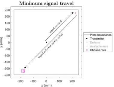
The choice of the length of the signals (number of timesteps) is fundamental: the minimum length must be the time that the emitted signal needs to travel to the farthest defect (with respect to the emitter) and to be reflected back to the farthest receiver (with

N o rm a lis ed a m p lit u d e

(41)

respect to the defect), as depicted in Fig. 13. To comply with this requirement, this distance was set to be 1.5 times the diagonal of the plate, thus:

𝑡𝑖𝑚𝑒𝑠𝑡𝑒𝑝 >1,5 ∙ 𝑑𝑖𝑎𝑔𝑜𝑛𝑎𝑙

V ∙ 𝑓 =

1,5 ∙ 2 ∙ 0,5

3282 ∙ 4𝑒 = 1293 (8)

Where 𝑓 is the sampling frequency of the signal. However, as previously mentioned, it would be advantageous to also include in the acquired signal some reflections from the boundaries of the plate, hence it was decided to acquire 2000 timesteps, i.e. an acquisition time of 0.5ms.

Fig. 14 shows the signals captured by the receiver placed at the three locations of Tab. 1 for a pristine plate at 20°C. Using the dispersion curves of Fig. 10 and the frequency of 300 kHz of the input signal, it is possible to estimate the first arrival time for both S0

and A0:

𝑡 =𝑑

𝑉 ; 𝑡 =

𝑑

𝑉 (9)

being 𝑑 the distance of the receiver from the emitter and 𝑉 and 𝑉 the group velocities of S0 and A0 respectively. Tab. 4 reports the results obtained by applying the

velocities of Tab. 2 in eq. (9).

(42)

Sensor D [mm] First arrival time [ms]

S0 A0

1 45 0,009 0,014

2 165 0,034 0,050

3 284 0,058 0,087

Tab. 4: first arrival times computed from dispersion curves data Fig. 14 also shows that:

 the farther the receiver from the emitter, the lower the amplitude of the intercepted signal;

 anti-symmetric mode A0 has a higher amplitude than the symmetric mode S0: this

is due to the fact that the excitation from the emitter is given in normal direction with respect to the plate, thus exciting almost exclusively A0 mode;

 the closer the receiver to the boundaries, the faster the arrival of the reflections;  looking at the envelope of the first wave packet arriving to the sensor it is possible

to confirm what expected from the analysis of the dispersion curves of Fig. 10: the excited A0 mode preserve its shape as it travels through the plate, hence

reducing the complexity of the received signal.

Fig. 14: signals captured by the receiver placed in the three chosen locations

N o rm a liz e d a m p lit ud e s

(43)

1.2. Pre-processing of the signals before

being fed to the ML algorithms

The numerical signals were processed prior to be fed to the ML algorithms in order to make them more realistic:

 the temperature effect on signals, which is one of the main issues when dealing with ultrasound-based SHM problems, can be mitigated by applying BSS [1] [2] technique;

 the signals obtained from the numerical simulations are not affected by instrumentation noise, thus an artificial noise is added in order to reproduce datasets with certain SNRs;

 the dataset must be properly divided into training, validation and test sets in order to effectively train all ML models

These 3 steps are now discussed in depth.

1.2.1 Baseline Signal Stretch (BSS)

The effect of temperature in the numerical model was already introduced in chapter 1.1.2. Three numerical signals received by the sensor number 1 from models at different temperatures are shown in Fig. 15:

 envelopes arrives at almost the same time since the distance between emitter and receiver is short. The main visible effect is the phase shift due to the different phase of the signal emitted in each of the three models;

 towards the end of the signal (Fig. 15, zoom B) the main visible effect is the different arrival time of the envelope in each of the three signals, due to the longer distance travelled by the propagating modes.

These distortions hinder the detection of reflections originating from defects. BSS technique is one of the most used temperature compensation approaches [1] [2]. A baseline signal is taken as reference and all the others are compressed or elongated in time to best fit the baseline signal (i.e. to reduce the RMSE of the signal obtained by subtracting the modified signal from the baseline). This method allows to obtain signals with equal time of flight (tof), independently from the temperature at which the signal is acquired. In this study the baseline signal was set to be the pristine signal at 45°C (in the middle of the range between 20°C and 69°C) for all the receivers; the results are reported in Fig. 16 that shows the improvement given by this transformation: in zoom A the temperature effect is still dominated by the phase change given by the temperature effect in sensors; in zoom B the signals are almost completely overlapped.

(44)

As explained in the next section, noise was added to the signals and it would be more realistic to apply BSS to the noise-corrupted signals rather than to the noise-less signals as done in fig. 15. However, since the disturbance due to the introduced noise is significantly smaller than the largest peaks of the signals, only negligible differences would be obtained by applying BSS to the noise-corrupted signals rather than to apply noise on the BSS-compensated noise-less signals. Since at each iteration of the study an entirely different set of noise was added to the signals, in order to save computation time it was decided to first compensate all the noise-less signals with the BSS method and hence to simply apply noise at each iteration to the compensated signals.

Fig. 15: signals taken at three different temperatures

N o rm a liz ed a m p lit ud e N o rm a liz ed a m p lit ud e N o rm a liz ed a m p lit ud e N o rm a liz ed a m p lit ud e N o rm a liz ed a m p lit ud e N o rm a liz ed a m p lit ud e