Anno accademico 2016/2017 Sessione III
ALMA MATER STUDIORUM - UNIVERSITÀ DI BOLOGNA
SCUOLA DI INGEGNERIA E ARCHITETTURA
DIPARTIMENTO DI INGEGNERIA DELL’ENERGIA ELETTRICA E DELL’INFORMAZIONE “Guglielmo Marconi”
DEI
CORSO DI LAUREA IN INGEGNERIA DELL’AUTOMAZIONE
TESI DI LAUREA in
Computer Vision e Machine Learning
LEARNING TO DETECT GOOD IMAGE
FEATURES
CANDIDATO RELATORE
Andrea Avigni Chiar.mo Prof. Luigi Di Stefano CORRELATORE Dott. Federico Tombari
III
ACKNOWLEDGEMENTS
I would like to express my sincere gratitude to my advisors Prof. Luigi Di Stefano and Dr. Federico Tombari for the opportunity they offered me and for their guidance and support in the development of the project and the preparation of the thesis.
In addition, I would like to thank the students of the CAMPAR of the Technical University of Munich, David, Keisuke, Christian and Iro, who helped me with the tools necessary for the thesis, and Pietro for his help in the writing of the thesis.
IV
TABLE OF CONTENTS
PAGE
ACKNOWLEDGEMENTS ... III LIST OF TABLES ... VI LIST OF FIGURES ... VII LIST OF SYMBOLS AND ABBREVATIONS ...XI RIASSUNTO ... XII ABSTRACT ... XIII
CHAPTER 1 INTRODUCTION ... 1
CHAPTER 2 LITERATURE REVIEW ... 4
2.1 Learning a Descriptor-specific 3D Keypoint Detector ... 4
2.1.1 Definition of the training set... 4
2.1.2 Design of the classifier ... 5
2.2 Temporally Invariant Learned Detector ... 6
2.2.1 Definition of the training set... 6
2.2.2 Design of the regressor ... 6
2.3 BRIEF and FREAK Descriptors ... 7
2.4 Neural networks ... 8
2.4.1 Artificial neural networks ... 9
2.4.2 Deep neural networks ... 10
CHAPTER 3 METHODS ... 13
3.1 Samples extraction and training of the classifier ... 13
3.1.1 Sampling and description ... 14
3.1.2 Matching ... 16
3.1.3 Positive and negative sample extraction ... 19
3.1.4 Features extraction ... 21
V
3.1.6 Training of the neural network ... 24
3.2 Validation ... 30
3.2.1 Training and test error ... 31
3.2.2 Precision-Recall curve ... 32
CHAPTER 4 RESULTS ... 34
4.1 Positive and negative sample extraction ... 34
4.2 Training ... 38
4.2.1 Random forest ... 38
4.2.2 Convolutional neural network ... 44
4.3 Test 46 4.4 Comparison with TILDE ... 54
CHAPTER 5 CONCLUSIONS AND FUTURE WORK ... 57
VI
LIST OF TABLES
Table 3-1 List of the parameters ... 14
Table 3-2. Score table initialization ... 18
Table 4-1. Speed comparison of all the combinations of parameters ... 34
Table 4-2. Comparison of all the combinations of parameters ... 45
Table 4-3. Thresholds and average number of keypoints for every webcam ... 49
Table 4-4. Average speed of the random forest applied to one image of the dataset (note that when using FREAK a sampling rate of 2 is applied to the image)... 50
VII
LIST OF FIGURES
Figure 1-1. SIFT detector ... 1
Figure 1-2. FAST detector ... 1
Figure 1-3. Description matching ... 2
Figure 2-1. Overview of the definition of positive samples ... 4
Figure 2-2. Feature extraction... 5
Figure 2-3. TILDE positives extraction ... 6
Figure 2-4. BRIEF pairs ... 7
Figure 2-5. FREAK test points ... 8
Figure 2-6. Some digits from MNIST... 8
Figure 2-7. Simple neural network architecture ... 9
Figure 2-8. ReLU ... 10
Figure 2-9. Convolution ... 11
Figure 2-10. Max pooling ... 12
Figure 2-11. LeNet architecture ... 12
Figure 3-1. Images from AMOS (a) and Panorama (b) datasets... 13
Figure 3-2. Image sampling and computation of the descriptors ... 14
Figure 3-3. Keypoints removal: (a) before the computation of the descriptors, (b) after ... 15
Figure 3-4. Matching types: straight matching (a) and cross matching (b) ... 16
Figure 3-5. Some images from the Chamonix training dataset ... 17
Figure 3-6. Matching error ... 18
Figure 3-7. Fixed threshold (a) and dynamic threshold (b) ... 19
Figure 3-8. Positive (black) and negative (white) locations: (a) Sampling rate = 5. (b) Sampling rate = 3, with non-maxima suppression ... 20
Figure 3-9. Example of positive (black) and negative (white) locations with sampling rate = 10 and negative radius = 10 ... 21
Figure 3-10. Some of the 32x32 patches used to train the CNN ... 22
VIII
Figure 3-12. Example of problems with clouds: Frankfurt webcam using a random forest trained
on Chamonix dataset ... 23
Figure 3-13. Example of one-hot encoding ... 24
Figure 3-14. Architecture of the CNN ... 25
Figure 3-15. TensorBoard homepage ... 27
Figure 3-16. Cost function with (a) smoothing = 1 and (b) smoothing = 0 ... 27
Figure 3-17. Example of convolutions applied to an input patch ... 28
Figure 3-18. Example of upsampling ... 30
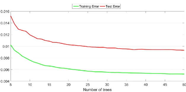
Figure 3-19. Example of training and test error with different numbers of trees ... 31
Figure 3-20. Example of 1 - Precision / Recall curve ... 33
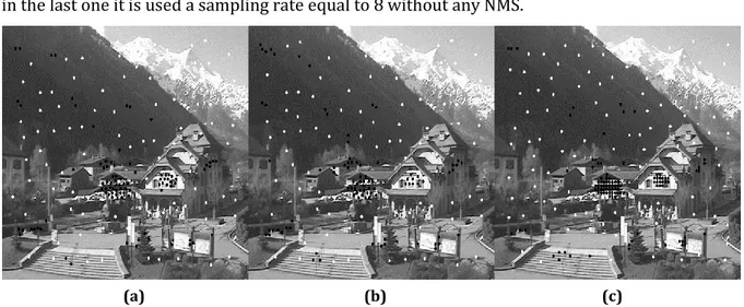
Figure 4-1. Comparison between sample extraction using BRIEF and a straight matching with (a) sampling rate 3, (b) sampling rate 5, (c) sampling rate 8. The black dots are positive samples while the white dots are the negatives. ... 35
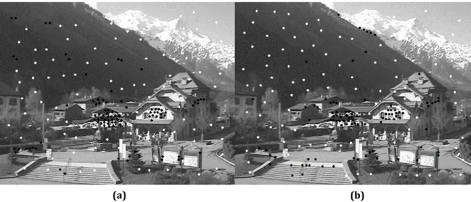
Figure 4-2. Positive (in black) and negative (in white) points obtained using (a) BRIEF description and (b) FREAK description ... 36
Figure 4-3. Positive (in black) and negative (in white) samples using BRIEF (up) and FREAK (down) ... 36
Figure 4-5. Positive (in black) and negative (in white) samples using the cross matching ... 37
Figure 4-4. Positive (in black) and negative (in white) samples using the straight matching ... 37
Figure 4-6. Positive (in black) and negative (in white) samples using the cross-random matching ... 38
Figure 4-7. Example of an xml file containing the descriptors used for the training of the forest ... 39
Figure 4-8. Training and test error when using a different value for the number of trees ... 40
Figure 4-9. Training and test error when using a different value for the depth of the trees ... 40
Figure 4-10. Training and test error when using a different value for the number of samples to be left at a node ... 41
Figure 4-11. Comparison between precision-recall curves obtained using the straight matching type and different sampling rates ... 41
IX
Figure 4-12. Comparison between precision-recall curves obtained using the cross-random
matching type and different sampling rates ... 42
Figure 4-13. Comparison between precision-recall curves obtained using different matching types ... 42
Figure 4-14. Comparison between precision-recall curves obtained using different descriptor types ... 43
Figure 4-15. Random forest prediction over a validation image ... 44
Figure 4-16. Comparison between a batch size of 50 (orange) and a batch size of 100 (blue) .... 44
Figure 4-17. Random forest prediction using FREAK descriptors on an image from the Frankfurt webcam ... 46
Figure 4-18. Random forest prediction using FREAK descriptors on an image from the Courbevoie webcam ... 47
Figure 4-19. Comparison between a random forest prediction using FREAK descriptors (up) and BRIEF descriptors (down) ... 48
Figure 4-20. Comparison between P-R curves obtained using FREAK descriptor and different predictive thresholds over the Courbevoie dataset ... 49
Figure 4-21. Comparison between P-R curves obtained using BRIEF descriptor and different predictive thresholds over the StLouis dataset ... 50
Figure 4-22. CNN classifier applied to an image from the StLouis webcam ... 51
Figure 4-23. CNN classifier applied to an image from the StLouis webcam ... 51
Figure 4-24. Comparisons between random forest and CNN with both BRIEF and FREAK descriptors over the Mexico sequence ... 52
Figure 4-25. CNN keypoint detection over an image from the Mexico sequence ... 53
Figure 4-26.CNN keypoint detection over an image from the Courbevoie sequence ... 53
Figure 4-27. Keypoint detection using TILDE on an image from the Mexico sequence ... 54
Figure 4-28. Keypoint detection using the random forest on an image from the Mexico sequence ... 54
Figure 4-29. Keypoint detection using the CNN on an image from the Mexico sequence ... 55
Figure 4-30. Comparisons between random forest, CNN and TILDE using BRIEF descriptor over the Courbevoie sequence ... 55
X
Figure 4-31. Comparisons between random forest, CNN and TILDE using BRIEF descriptor over the Mexico sequence ... 56 Figure 4-32. Comparisons between random forest, CNN and TILDE using BRIEF descriptor over the StLouis sequence ... 56
XI
LIST OF SYMBOLS AND ABBREVATIONS
SIFT Scale Invariant Feature Transform FREAK Fast REtinA Keypoint
BRIEF Binary Robust Independent Elementary Features TILDE Temporally Invariant Learned DEtector
AMOS Archive of Many Outdoor Scenes ANN Artificial Neural Network CNN Convolutional Neural Network
XII
RIASSUNTO
Gli algoritmi di feature detection allo stato dell’arte sono stati pensati per estrarre determinate strutture da immagini e per raggiungere un alto livello di ripetibilità dei punti salienti, ossia per rilevare gli stessi punti in immagini sottoposte a determinate trasformazioni. Tuttavia, questo criterio non garantisce che i punti trovati saranno ottimali durante la fase successiva: il matching. L’approccio sviluppato all’interno di questo lavoro è volto all’estrazione di punti salienti che massimizzino le prestazioni del matching in accordo con il tipo di descrittore scelto. Per fare ciò, un classificatore è stato addestrato utilizzando un insieme di descrittori “positivi” e “negativi” estratti da immagini sottoposte a trasformazioni definite in precedenza. Prima di tutto, le immagini utilizzate per l’addestramento sono state campionate e confrontate analizzando le distanze tra i descrittori ottenuti attraverso uno specifico procedimento. Successivamente, si è creato l’insieme dei campioni positivi prendendo i descrittori relativi a quei punti che hanno dato corrispondenze corrette durante la fase di matching. Contrariamente, punti campionati casualmente e sufficientemente distanti dagli esempi positivi sono stati classificati come negativi. Infine, i descrittori calcolati in corrispondenza delle posizioni positive e negative sono stati utilizzati per addestrare il classificatore, il quale, ricevendo in input nuove immagini, può definire autonomamente la salienza dei punti sulla base dei loro descrittori e ottenere, così, un insieme di posizioni chiave. Questo procedimento richiede, però, l’estrazione dei descrittori in ogni punto dell’immagine e ciò comporta un alto carico computazionale. Questo, insieme allo stretto legame che vincola il metodo di descrizione utilizzato in fase di training a quello utilizzato durante il testing, limita la performance del detector. Per evitare queste problematiche, l’ultima parte del lavoro di tesi si è concentrato sulla creazione e addestramento di una rete neurale convoluzionale, utilizzando come esempi positivi piccole porzioni di immagine centrate nei punti in grado di fornire corrispondenze corrette tra diverse immagini. Si sono infine analizzate le performance dell’algoritmo sviluppato confrontandolo con lo stato dell’arte su un benchmark pubblico di riferimento.
XIII
ABSTRACT
State-of-the-art keypoint detection algorithms have been designed to extract specific structures from images and to achieve a high keypoint repeatability, which means that they should find the same points in images undergoing specific transformations. However, this criterion does not guarantee that the selected keypoints will be the optimal ones during the successive matching step. The approach that has been developed in this thesis work is aimed at extracting keypoints that maximize the matching performance according to a pre-selected image descriptor. In order to do that, a classifier has been trained on a set of “good” and “bad” descriptors extracted from training images that are affected by a set of pre-defined nuisances. First of all, the images used for the training have been sampled and matched by comparing the descriptor vectors obtained using a specific descriptor method. Then, the set of “good” keypoints is filled with those vectors that are related to the points that gave correct matches. On the contrary, randomly chosen points that are far away from the positives are labeled as “bad” keypoints. Finally, the descriptors computed at the “good” and “bad” locations form the set of features used to train the classifier that will judge each pixel of an unseen input image as a good or bad candidate for driving the extraction of a set of keypoints. This approach requires, though, the descriptors to be computed at every pixel of the image and this leads to a high computational effort. Moreover, if a certain descriptor extractor is used during the training step, it must be used also during the testing. In order to overcome these problems, the last part of this thesis has been focused on the creation and training of a convolutional neural network (CNN) that uses as positive samples the patches centered at those locations that give correct correspondences during the matching step. Eventually, the results and the performances of the developed algorithm have compared to the state-of-the-art using a public benchmark.
1
CHAPTER 1
INTRODUCTION
The paradigm of local features has been widely studied from the early 2000s and it is still matter of discussion among researchers all over the world. The most “interesting” points of an image, also known as keypoints, are the pivots of such paradigm that is based on three main steps: detection, description and matching. Finding corresponding points between images is a fundamental task for many applications, like object detection, SLAM (Simultaneous Localization And Mapping), augmented reality and many others.
The first step is the local features detection which searches across the images for points or shapes that are likely to be found in other images. In order to accomplish this requirement, it is necessary to define a priori what is the most distinctive characteristic that a group of pixels should deploy. For instance, the so called “Canny Edge Detector” [1] is one of the most popular algorithm when it comes to finding points between two image regions, whereas the method proposed by Chris Harris and Mike Stephens [2] relies on a function that gives negative values in case of edges, positive values for corners and zero for flat regions. Finally, algorithms exist that aim at the detection of regions of images that differ in properties. For instance, SIFT [3] (Scale Invariance Feature Detection) searches for the extrema of the Difference of Gaussian, i.e. the difference between several images obtained by applying a Gaussian filter with an increasing smoothing effect to the same initial image. The maximum is sought in space (8 pixels) and in scale (18 pixels).
Another example of feature detector is FAST [4] (Features from Accelerated Segment Test), where a point p is identified as keypoint if enough points on a circle centered at p all have a higher or a lower intensity with respect to the intensity of the central point.
Figure 1-1. SIFT detector
2
State-of-the-art keypoint detectors, such as the abovementioned ones, have been designed in order to achieve a high keypoint repeatability, which means that salient points have to be found in different views of the same scene despite possible transformations applied to the image, and in order to find specific shapes. For instance, Canny edge detector can find edges only, while Harris detector can identify both edges and corners. SIFT and FAST, instead, are specialized in both corners and blobs (regions).
After having detected the salient points over the images, they must be described so that it is easy to find them afterwards. This second step is aimed at creating a vector of numbers, by looking at the neighborhood of the point, in such a way that the result will have a high distinctiveness, i.e. it will capture the salient information around the keypoint, and a high compactness, namely low memory occupancy. Finally, as shown in Figure 1-3, corresponding points must be found in order to localize the salient point of the first image into the second one.
Each element of the paradigm of local feature must work well itself; for instance, a measure of goodness for detectors is the repeatability, i.e. how many times the same point is detected over a sequence of different images of the same scene. However, the most important aspect is the whole detector-descriptor-matching pipeline output and this is only partially related to the repeatability of the detector. As previously mentioned, state-of-the-art keypoint detectors try to maximize the keypoint repeatability, but this does not guarantee that the points that have been found will be the optimal ones during the subsequent steps (description and matching). The idea behind this thesis is to create a keypoint detector that searches over input images for those points that will yield highly distinctive description vectors. In order to do that, a classifier has been trained so that it will judge each pixel of an unseen input image as a good or bad candidate for driving the extraction of a set of keypoints. This thesis work is a follow-up to a recently proposed paper titled “Learning a Descriptor-specific 3D Keypoint Detector” [9] that uses the same idea applied to the
3
3D case. As an alternative, in order to decouple the detector method from the choice of a specific keypoint descriptor, a convolutional neural network has been trained so that it is no longer necessary to define a priori the feature type.
The research approach of this work has been mainly developed using C++ and OpenCV along with already existing images datasets, namely some of the ones used as training set in “Temporally Invariant Learned Detector” (TILDE) [6], that is composed by images from the “Archive of Many Outdoor Scenes” (AMOS) [13] and panoramic images, in addition to the “Oxford” [14] and “EF” [15] datasets. For the last part, regarding the neural network modeling, Python and TensorFlow have been used.
The work is organized as follows: Chapter II describes the literature, in particular the paper TILDE, in which a classifier is trained using highly repeatable keypoints, and the paper “Learning a Descriptor-specific 3D Keypoint Detector”, since these are the papers that are mostly related to this work; at the end of this chapter a brief explanation is also given about the two keypoint description methods used and some hints about how neural networks operate. Chapter III explains in detail the methods used in this work for the extraction of the positive and the negative samples, the training step and the testing procedure; Chapter IV shows the experimental setup and the qualitative and quantitative results obtained from the comparison between this method and the one proposed in TILDE; eventually, Chapter V gives some conclusions and an overview of the future work.
4
CHAPTER 2
LITERATURE REVIEW
The keypoint detectors that have been described in the introduction are all different and each one has its own specific algorithm; however, it is possible to split them in two main groups: the handcrafted keypoint detectors and the learned keypoint detectors. The former tries to overcome all the possible transformations an image can be subject to by looking for specific image structures, whereas the latter uses machine learning techniques to make the algorithm understand which are the most important features to be sought, starting from an initial input training set. For instance, SIFT [3] uses the Difference of Gaussian function as saliency function and it searches for the maxima of such function, while TILDE [6] and “Learning a Descriptor-specific 3D Keypoint Detector” [9] rely on previously trained classifiers for the keypoint detection. We will focus on these two papers.
2.1 Learning a Descriptor-specific 3D Keypoint Detector
The standard approach in 2D and 3D keypoint detection involves local saliency functions that give relevant locations at their maxima. However, this is not related to the quality of the descriptor that will be computed at those coordinates. In this work, it is proposed to train a classifier with points from a point cloud image that gives correct matches over a sequence of partially overlapping 2.5D views of the same 3D object.
2.1.1 Definition of the training set
The classifier that the authors want to train needs two separate sets: the positive sample set and
the negative one. The extraction process of the positive sample points from the 3D image is shown in Figure 2-1 and it is composed of five main steps. First of all, let {Vi} be the N partially overlapping
views of the 3D object and let νi be the set of views partially overlapping with a view Vi. Then, in
5
the third step, for every view Vi the SHOT [10] descriptor is computed at each point and the
nearest neighbor SHOT descriptor in the overlapping view Vj is sought. Now the list of matched
points is analyzed and if the match is correct the point is added to the list of positive samples, otherwise it is removed from the list. In the fourth step the list of positives is refined by checking if the positive samples can be robustly matched also in the other overlapping views. On the other hand, the set of negative points is randomly sampled from the set of points not included in the positive set.
2.1.2 Design of the classifier
The chosen classifier is a Random Forest [5], essentially because it is one of the fastest classifiers and, since it must be applied to every point of the point cloud, the speed is one of the most important elements to be considered. When using a classifier, a feature must be defined; usually, simple binary features such as intensity differences are used, but they need a local reference
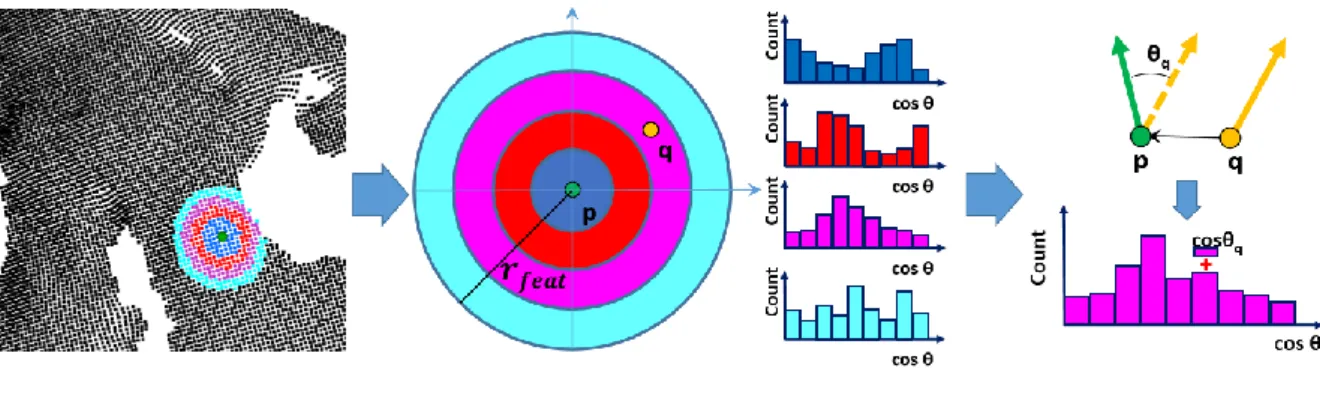
frame to be defined, in order to preserve rotation invariance, and this increases the computational load. In this work, the authors store the cosine of the angle between the normal at the reference point p and the normal at every point within a radius rfeat in several histograms and use them as
features. Since the histograms are computed for spherical shells, they are rotation invariant and then the local reference frame is no longer needed. Finally, when the classifier is applied to unseen input point clouds, the number of trees Tp that identify a point as a keypoint is counted and if the
score Tp/T, where T is the total number of trees, is higher than a minimum score smin ≥ 0.5 and it
is the highest value in a neighborhood of radius rnms, then the keypoint is validated.
The procedure that has been used in this paper for the extraction of the positive samples is equal to the one used in this thesis work, except for the use of different invariant transformations. Indeed, in the 3D case, these transformations are 3D viewpoint changes, while in the 2D case, which is the one explored in this work, they are illumination changes.
6
2.2 Temporally Invariant Learned Detector
A great variety of keypoint detectors has been proposed since the 1980s and, even if they exhibit excellent repeatability with scale and viewpoint changes, they are all very sensitive with respect to illumination changes. In this work, the authors train a regressor using points that have been consistently found over a sequence of images that present drastic illumination changes due to different weather conditions.
2.2.1 Definition of the training set
The dataset that has been used for the training step is composed of two main groups:
• some images from the “Archive of Many Outdoor Scenes” (AMOS), that is a dataset that collects pictures from fixed webcams all over the world; the images are taken at different times of the day and different seasons;
• some panoramic images from a fixed camera located at the top of a building.
The authors trained the regressor on the images of one fixed webcam and then tested on the others along with further images from different datasets. After having collected a certain number
of images from one webcam, they applied SIFT detector to every image and they kept the 100 best repeated locations. Then, the set of positive samples is filled with the patches around these points even in the images where they have not been detected. The negative locations, instead, are just points far enough from the keypoints used to create the set of positive samples.
2.2.2 Design of the regressor
The features that the authors of the paper used are the three components of the LUV color space, the vertical and horizontal gradients and the gradient magnitude computed at each pixel of the
7
patches. Since the detector will be applied to each location of the images, the speed of the algorithm is a crucial element. Thus, here a fast regressor is used, that applies only simple convolutions and pixel-wise maximum operators:
𝐹(𝑥; 𝜔) = ∑ 𝛿𝑛maxm=1𝑤 𝑀
𝑛𝑚𝑇 𝑥 𝑁
𝑛=1 , (2-1)
where x is a vector of image features extracted from the patches, ω is the vector of parameters of the regressor and it can be decomposed in a combination of linear filters wnm and a set of
parameters δn. The linear filters are the elements to be learned through an optimization function
over the training images and they can be approximated as a linear combination of separable filters. At the end two different methods can be used: TILDE-P, that uses the original filters and TILDE-P24 that uses 24 separable filter in order to speed up the process.
As already mentioned, TILDE is probably the most related to this thesis work in the sense that the authors used a machine learning technique to learn a 2D keypoint detector starting from a set of positive and negative samples. As a consequence, the datasets used in this work for the training and testing steps are the same.
2.3 BRIEF and FREAK Descriptors
“Binary Robust Independent Elementary Features” [7] is a description method that, when applied to a certain image patch around a point of interest, returns a binary descriptor, where binary means that is composed by 0s and 1s only. When we want to find correspondences among points of more images, the comparison between such type of descriptors can be very convenient with respect to non-binary vectors, because it allows the use of the Hamming distance and, then, a considerable speed-up of the matching step. SIFT descriptor would require a conversion from the standard vector to the binary equivalent if the Hamming distance is being used, whereas BRIEF extracts a binary value directly from the patch itself. Indeed, the idea behind BRIEF is to pick random points from a Gaussian distribution and test them. The Gaussian distribution has the following form:
(𝑥, 𝑦) ~ 𝑖. 𝑖. 𝑑 𝐺𝑎𝑢𝑠𝑠𝑖𝑎𝑛 (0, 1
2∗𝑆∗ 𝑆
2) , (2-2)
where S is the patch size. The test gives as result 1 if the intensity of the pixel x is lower with respect to the intensity of y and 0 otherwise. If we proceed through many pairs we will end with a string of binary values that is the BRIEF Descriptor.
8
This type of descriptor, tough, is very sensitive to rotation; indeed, if the image is rotated by more than a few degrees, the matching performances of BRIEF falls off
sharply. Randomly picking up points from a Gaussian distribution is not the only possible choice to select the locations that are processed by the test. The authors of the work “Fast REtinA Keypoint” [4] tried to understand which are the best pairs to be used for the test by analyzing the human visual system. Figure 2-5 shows the comparison between the points used for the test along with their Gaussian blur radius and a
human retina region responsible for sharp central vision that is composed by three main elements: fovea, parafovea and perifovea. Similarly to what happens in our eyes, the outer points (perifoveal area) are the first to be analyzed because they are the most discriminative locations, while the central points (foveal area), that are the least blurred ones, are the last pairs to be tested. Regarding rotation invariance, the orientation is estimated by summing the local gradients of some pairs that are symmetric with respect to the center of the patch.
2.4 Neural networks
Neural networks are one of the most used machine learning techniques that have become very popular in the last few years thanks to the decrease of hardware prices and to more performant GPUs (Graphic Processing Units) for personal use. Neural networks with different architectures are used for countless applications, like speech recognition, understanding of biological data, character text generation and many others. Concerning the computer vision field, deep learning, i.e. the branch of machine learning that uses neural networks, is widely used for object classification, colorization of black and white images, medical images segmentation and so on. The human visual system can perform extremely complex image analysis. This ability is the
consequence of millions of neurons linked by billions of connections inside the five visual cortices of our brain. Our efficiency in visual pattern recognition is the result of a long training process that last many years and that teaches us how to perfectly use our powerful eyes. As a consequence, it is not so easy to imitate the human visual system in all its complexity and to carry out a proper training procedure. Figure 2.6, which shows some handwritten digits from the MNIST (Mixed National
Figure 2-5. FREAK test points
9
Institute of Standards and Technology) dataset, is an example of how easy is for the human brain to recognize such images as meaningful information. If we want to create a computer program capable of understanding which number is in front of a camera, though, it would not be easy at all. For instance, we could try to identify the digit “1” by assuming that a fundamental characteristic is the bar at the bottom of the stroke. The problem would be that with such a precise rule it can be hard to identify other “ones” that deploy different features and if we start adding exceptions we could end up in many wrong classifications. Therefore, we need something more powerful and, at the same time, flexible with respect to small variations.
2.4.1 Artificial neural networks
Artificial neural networks (ANNs) are a machine learning technique that can infer specific characteristics of an input training sample and then seek them during the testing step. When we use this algorithm, we do not need to define a priori which shapes identify a sample as belonging to a certain class; indeed, it is the network itself that will learn how the elements of the training data associated with a label must be distributed. For instance, in the case of handwritten digit classification, the feature to be learned is the distribution of pixel intensities over the images.
Figure 2-7. Simple neural network architecture
ANNs are inspired by and loosely based on biological neural networks. Indeed, the idea behind the functioning of ANNs is to use many linked elementary units in order to achieve high performances when dealing with complex tasks. All these interconnected neurons exchange information and update every time a new training sample is injected along with its label. In
10
practice, the neural network should learn a set of weights and biases that, when combined with the input will give us back a probable prediction of a certain label as output. For instance, if our input is x we must initialize the set of weights and biases and then, using the formula
ŷ = 𝑊 ∗ 𝑥 + 𝑏 (2-3) we compute the predicted output and we compare it to the real value of y, that we know since all the training data come with their own labels. The aim of this procedure is to minimize a cost function time by time, by updating weights and biases at every step of the training. This optimization problem can be solved in several ways, for example using gradient descent, stochastic gradient descent and some others. The output of every node is the result of a linear process and, even if its efficiency is high, especially using GPUs and simple matrix operations, a non-linear component is necessary, otherwise the network would lose the ability to model non-linear patterns. Therefore, the output of the linear equation (2-3) is processed by the so-called activation function. Figure 2.8 shows an example of activation function called ReLU (Rectified Linear Unit) that gives y=0 if x is negative and y=x if x is positive. The advantages of this function are that it is differentiable everywhere except in zero and its derivative is very simple: zero if x is negative and 1 if x is positive.
A simple ANN (for example with only 2 layers) can approximate a large variety of models but it uses many nodes and it needs many training images in order to get acceptable values for every parameter. A good solution to these problems is to increase the depth of a network by adding many layers and to reduce the number of nodes per layer.
2.4.2 Deep neural networks
A deep neural network is a very powerful tool that uses many layers of abstraction to infer features of some input signals. The structure of such network is composed by several layers one on top of the other in a way that every layer tries to elaborate the outputs of the previous layer in order to get the best possible prediction for the output. When using deep network, the number of inputs used for the training procedure can be lower with respect to the simple ANNs, and this can easily lead to overfitting, namely the problem of having a too complex model that can hardly work in a general case. In order to solve this problem, it is used the so-called regularization and a possible technique that has been recently proposed is called dropout. The idea behind this
11
technique is to deactivate 50% of the nodes during each iteration of the training step such that the algorithm can never rely on the same inputs.
Deep neural networks, like ANNs, can be developed using many possible architectures that change depending on the depth of the network and on the type of layers used. When dealing with images, a widely used types of layers are convolutional layers and pooling layers, that can be combined together in order to analyze the spatial information of an image. The main reason it is possible to use this approach with images is that pixels can share their weights to reduce the degrees of freedom of the model.
A convolutional layer is a layer in which a simple square filter is applied as a sliding window over the images. The main parameters here are the dimension of the filter, the stride to use, i.e. how many pixels must be skipped between two filters and whether the size of the image after the convolution should remain constant or not. When applying convolutions on the borders of an image, some pixels could be missing since the filter is only partially overlaid to the image. In this case, we have two possibilities:
• use some padding (for instance zero-padding) in order to get some information also on the edges of the images;
• apply the convolution without any padding and skip all the locations where the filter could not be computed. In this case the dimension of the images will not remain constant. The output of this layer will be, then, an image with the same dimension (if padding is present) and a certain depth that indicates the number of channels. Figure 2.9 shows an example of convolution with a stride of 1 along all the directions. In this case the padding is not used, thus, the final image has a smaller dimension, more specifically, one pixel is “lost” on one boundary and one on the other boundary.
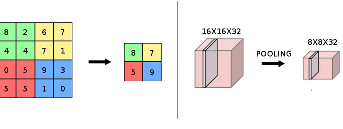
Another type of layer is the pooling layer that is used to reduce the spatial dimension but it keeps the same number of channel of the input image. The downsampling is carried out by taking some information from a cluster of pixels using a specific criterion. For instance, Figure 2.10 shows the so-called max pooling layer, that takes the maximum intensity among the ones of the pixels within
12
a sliding window. The parameters to be set here are the size of such sliding window and the strides.
As already mentioned before, many architectures can be implemented by changing the parameters of the layers and the number of layers itself. Figure 2.11 shows the so-called “LeNet” architecture, created in 1998 by Yann LeCun for handwritten letters recognition.
Figure 2-10. Max pooling
13
CHAPTER 3
METHODS
3.1 Samples extraction and training of the classifier
The procedure that has been used in this thesis is the same as in the previously mentioned “Learning a Descriptor-specific 3D Keypoint Detector”; indeed, the set of positive samples has been extracted from those points that gave a good correspondence during the matching between images of the same scene affected by specific transformations. In the 3D case, these transformations were 3D viewpoint changes, while here the viewpoint is always the same, but the images have acquired under different lighting conditions. Since this work is aimed at learning features from 2D images, the most relevant comparison that can be performed is with TILDE and, in order to make an even comparison, the dataset used here is the same of the one used in TILDE, for both training and testing. As already mentioned, the training dataset is composed by some images from the “Archive of Many Outdoor Scenes” (AMOS) dataset and panoramic images collected by the authors of TILDE, while the testing dataset is composed again by some images from AMOS and panorama.
(a) (b)
Figure 3-1. Images from AMOS (a) and Panorama (b) datasets
The whole procedure is developed through many small steps and each one of them needs specific parameters to be tuned. First of all, all the images of the training dataset are sampled and a descriptor is computed at every location; then, a matching step is performed and a table containing information about how many times a point has given a correct match is created; finally, the points are sorted from the ones with the highest goodness score down and the best ones are kept as positive sample locations. The set of negative samples is randomly sampled over the images in such a way that every point is far enough from both the already computed positives and the other negatives. In one of the two approaches used in this work, the features that will be used during the training of the classifier are vectors of description computed at the positive and
14
negative locations of every image of the training dataset, that are stored into vectors and will be used later. In the other case, with CNNs, it is not necessary to determine a priori the features that we need to feed because the neural network can learn these features autonomously, therefore the only thing we need from the locations detected by the matching procedure is the distribution of the intensities around them. Table 3-1 shows all the possible parameters that are combined and compared in order to determine which is the best arrangement to be used for the first step of this keypoint detector. The extraction of positive and negative samples is, of course, used in both random forest approach and CNN approach. The comparison will take place during the validation step and it will involve also other settings related to the classifier. In the next sections, the steps for the positive and negative samples extraction are explained in detail.
Table 3-1 List of the parameters
SAMPLING RATE 3 5 8
DESCRIPTOR TYPE BRIEF FREAK
MATCHING TYPE STRAIGHT CROSS CROSS-RANDOM
3.1.1 Sampling and description
The first important step is the training images sampling. Indeed, we need a set of points that will be compared to the others belonging to the remaining images of the dataset. Even if the sample extraction and the training of the classifier are both offline processes, meaning that they can be computed before the application of the keypoint detector to the test images, the speed of the whole process is important in practice. On the other hand, if we speed up the process by applying
a very low sampling rate, many points would be discarded and the number of positive candidates would be too low. To sum up, a dense sampling would be better in terms of quality of the positive
15
samples, but very slow, while a high sampling rate would make the process fast but not very precise.
The main parameters to be set here are two: • the sampling rate of the input images; • the descriptor to be used.
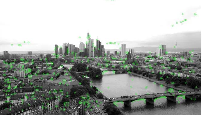
For the latter, while both detector and descriptor are included in the SIFT procedure, descriptor methods like “Binary Robust Independent Elementary Features” (BRIEF) [7] and “Fast REtinA Keypoint” (FREAK) [8] do not have an already integrated detector. The choice of the description method in this step must be the same during the final testing step when using the random forest, because if we train a classifier to recognize a specific pattern that is related to a certain descriptor type it will not recognize vectors created in a different way. It is possible to note in Figure 3.2 that many points on the borders are missing; the reason is that when the descriptor vectors are created, as already mentioned in Chapter 2, the intensities of many points around the central one (in this case the sampled point) are compared by looking at their intensities and if one or both points happen to be outside the image a problem occurs. In this case the point of interest is skipped and it is removed by the set of keypoints, but this aspect strongly depends on the choice of the description method.
In the case of CNNs, the problem of computing vectors of description before the testing procedure is not important since the features are inferred directly by the network. However, this first step has two purposes: the localization of the points that should be good for the training procedure and the extraction of the descriptors that will be used later when training the random forest. The former aim is common to both the random forest and the CNN and it needs anyway the computation of the descriptors in order to perform the matching procedure; thus, the problem of missing keypoints near to the boundaries cannot be avoided. The CNN, though, deals with patches
Figure 3-3. Keypoints removal: (a) before the computation of the descriptors, (b) after
16
and, even if there are no intensity differences, it could be possible that a portion of some patches covers an area that exceeds the boundaries of the image. Since we are discarding some points that are far enough from the borders, it will be always possible to extract all the patches centered at those points.
3.1.2 Matching
The second step is the matching, in which all the descriptors of two images are compared in order to find the best correspondences. This is the main difference with respect to TILDE, because, while TILDE extracts the best locations by applying an already existing keypoint detector and it labels a point as positive if it can be consistently found over the sequence of images, here a point is good only if it gives many times a good correspondence. In this specific case, since all the training images are already aligned, a good correspondence means that a point on the first image of a compared pair must point to a location in the second image of the pair with exactly the same coordinates. If it was not the case and similarity transformations were applied, a perspective matrix would have been needed in order to find the correct position.
The procedure to follow in order to find the positive locations can be various and the main parameter to decide here is which images will be compared. As already mentioned before, the used dataset is the same of TILDE, in which 100 images from the same webcam form the training set. Of course, the best solution would be to perform a cross matching between all the possible
Figure 3-4. Matching types: straight matching (a) and cross matching (b)
17
pairs of a training dataset, but it would require a lot of time. A workaround to this problem is to perform the matching step only over a subset of images from the training set and then extract the descriptors from the whole set, but this forces us to choose the images to use. This decision is very important since a wrong choice of the images could lead to favor specific features. For
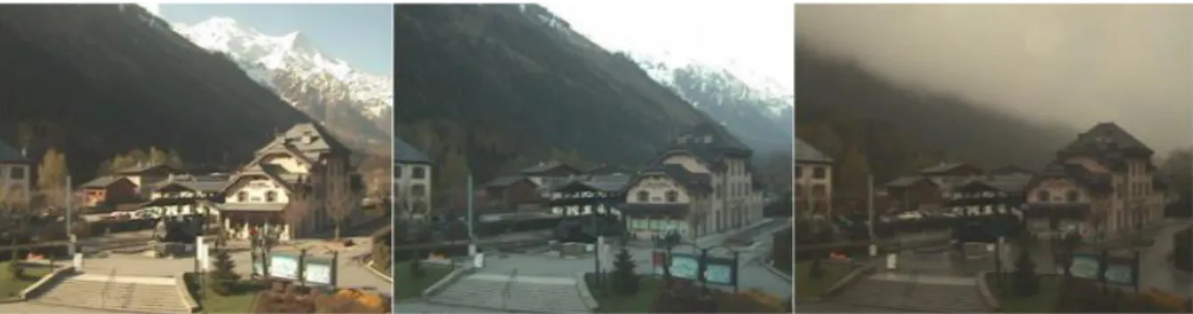
instance, Figure 3.5 shows a comparison between 3 different images of the same scene under different illumination and weather conditions. It is easy to note that if images with the same illumination and weather of the third image are not present among the images that must be compared, some points of the mountains in the background could be detected as positive and the final result could be biased. On the other hand, checking all the images and trying to manually hardcode the dataset could be very time wasting. A possible solution, then, is to inject randomness and let it decide for us. In this work three possibilities have been developed:
• a match between the descriptors of the first image of the dataset and all the others (straight approach);
• a match between pairs of images from a subset of the dataset composed by the first 30 images of the dataset (cross approach);
• a match between every image of the dataset and a subset of the dataset (cross-random approach).
In the first case the number of combinations is obviously smaller; indeed, if N is the number of images inside the dataset, N-1 matchings will be necessary, while in the cross matching case the procedure must be executed 𝑁!
𝑘!(𝑁−𝑘)! times, where k is 2 since every comparison is between 2
images only. In order to keep the sample extraction time almost constant, N must vary depending on the matching type we want to use. In the “straight” matching, 100 images have been used, exactly like TILDE, whereas, in the cross matching, 15 and 30 images have been used, resulting in 105 and 435 comparisons respectively. In the last case, every image of the training set is compared to some randomly chosen images, thus the number of comparisons depends on the times a random number, associated to an image, is chosen. A possible negative drawback here is
18
that randomly choosing a number does not guarantee that images like the third one of Figure 3-5
are chosen and this can affect the final positions of the positive samples. The main parameter to be set here is the descriptor type, that can be either BRIEF or FREAK, but also the matching algorithm is important; indeed, once the descriptors have been extracted around the points, the way in which they are compared can affect the final result. The tested alternatives are the Brute-Force Matcher, that takes the descriptor of one feature and compares it to all the others, and two matchers from the “Fast Library for Approximate Nearest Neighbors” [11] that use KDTree and Locality Sensitive Hashing. These two last methods are very fast in case of large dataset and for high dimensional features, but, since this is not the case, they are slower with respect to Brute-Force Matcher.
The objective of this matching step is to fill a table with information about the “goodness” of every point in terms of matchability. This table is initialized as shown in Table 3-2, where X and Y are
Table 3-2. Score table initialization
the coordinates of the sampled points, ID is necessary to identify every keypoint and the score is a value that indicates how many times a point has given a correct match over the sequence of images. When the first descriptor matching is executed, every point of the list of matches is checked and if the corresponding point given by the matching algorithm is in the correct position, where correct means in the same position of the first point of the pair, then the location coordinates are stored in a vector. It is important to note that a small matching error (1 or 2 pixels) is accepted and then a point gives a correct correspondence even if it is not exactly at the right position.
X Y ID SCORE
0 0 1 0
0 Sampling rate 2 0
… … … …
Max width Max height Max ID 0
19
At the end of this step, every positive location of the vector is sought over the score table and its score is increased by 1
𝑇𝑜𝑡𝑎𝑙 𝑛𝑢𝑚𝑏𝑒𝑟 𝑜𝑓 𝑐𝑜𝑚𝑝𝑎𝑟𝑖𝑠𝑜𝑛𝑠 that, in the case of straight matching, is equal
to 1
𝑁−1 , where N is the number of images, while in the case of cross matching is 2
𝑁(𝑁−1) since the
number of comparisons is 𝑁!
2(𝑁−2)! . The last case, namely the cross-random approach, is slightly
different because the score of a positive point is increased by 1
𝑁∗𝑖𝑚𝑔𝑠𝑇𝑜𝐶𝑜𝑚𝑝𝑎𝑟𝑒 , where imgsToCompare is how many random numbers are extracted for every image. When a point gives a correct correspondence, its location is updated and, as already mentioned before, no similarity transformation is needed since the training set is already aligned.
3.1.3 Positive and negative sample extraction
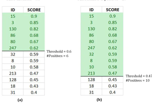
At this point, every location of the image has its own score that tells us how good the descriptor is, around those points to be matched later. In order to choose the best points, we have two possibilities: set a threshold on the scores and take all the points above that threshold or sort out all the points of the table from the one with the highest score and use a dynamic threshold that,
starting from 1, keeps decreasing until the number of points with a score higher than the threshold is greater than a predefined value. In the first case, when we set the threshold to a certain value, for instance 0.6, we do not know how many points will be found later and this can
Figure 3-7. Fixed threshold (a) and dynamic threshold (b)
20
be very bad because we could get either too many or too few points. For example, if a sequence of images is not affected by strong transformations, all the sampled points of the images can get a very high score and, with a low threshold, they could be all labeled as positive samples and during the testing step this results in a very low selective keypoint detector. Moreover, if the positive samples distribution is too dense, when the negative samples will have to be randomly picked, it will be hard to find points that are far enough from the good sample locations. On the other hand, if the dynamic threshold is used, the minimum number of positive samples that we want must be chosen beforehand, but the threshold changes and decreases as long as enough points are selected. This could result in a set of positive samples with a very low score that will have a bad influence on the final classifier. In this work, the dynamic threshold approach is used during the positive extraction procedure and the afore-mentioned problem does not exist anymore since the images suffer from illumination changes and not from similarity transformations, which means that many points can get a high score. Later in the process, during the testing step with random forests, will be necessary to decide which approach to use between the fixed and the dynamic threshold, and the best solution will be a fixed threshold since it is possible to adjust it before the real use of the algorithm.
The sampling rate defined during the first step of the process, when the images are sampled, could discard many points that could get a high matching score during the second step. As already mentioned, the best solution would be to analyze every pixel so to be sure that no good locations are left behind. However, this approach would require a lot of time and moreover, the OpenCV library, used in this thesis, does not allow to fill the set of training descriptors with more than 262144 items, limit that is easily reached by images like the one in Figure 3-8. Another important
Figure 3-8. Positive (black) and negative (white) locations: (a) Sampling rate = 5. (b) Sampling rate = 3, with non-maxima suppression
21
problem associated with the dense sampling is that many points of the same area can be detected as positive and this can lead the process to an extraction of many descriptors (in case of random forests) or patches (in case of CNNs) that are too similar.
Having a large variety of training data is fundamental for a good estimation because, otherwise, the algorithm cannot learn enough features and its predictions are not precise. In order to spread the points and cover a wider surface, the points are sorted from the one with the highest matching score to the one with the lowest. Then, starting from the first point, the locations around its coordinates within a certain radius are checked and, if their scores are lower with respect to the central one, they are discarded from the list of positives. Figure 3-8(a) shows an example of positive samples extraction with a sampling rate of 5 pixels without any improvement, while
Figure 3-8 (b) shows a training image with a sampling rate of 3 pixels and the previously explained technique with a radius of suppression equal to 6 pixels. Since the sampling rate is 3 pixels, having a radius of suppression equal to 6, 7 or 8 pixels does not make difference, because it is not possible to find a sampled pixel between the 6th and the 8th pixels.
3.1.4 Features extraction
When the final set of positive locations is complete, the features set that will be used for the random forest training is formed by all the descriptors computed at the positive locations over
every image of the training dataset, even in those where a certain location did not give a correct
Figure 3-9. Example of positive (black) and negative (white) locations with sampling rate = 10 and negative radius = 10
22
match during the previous step. Regarding the CNN, instead of the descriptors set, a set of patches extracted from the area around the selected positive and negative points is used.
The negative locations are randomly picked from the images in such a way that they are far enough from every positive location and every negative location.
Basically, a pair of integers are randomly sampled within a range defined by the width and the height of the images of the dataset; then, they are compared to the coordinates of the positive samples and if they are far enough from every positive location they are labeled as non-positive locations. In order to have a large variety of negative samples, the non-positive coordinates are also compared to all the points that are already inside the negative samples set and if the distance is greater than a certain value they can be inserted into the negative samples set. Figure 3-9 shows an example where the sampling rate is 10 pixels and the negatives (white dots) must have at least a distance of 10 pixels from both the positive and negative locations. In this thesis work the negative radius will be equal to 30 pixels. Using the random forest trained with the
descriptors computed at the positive and negative locations is more efficient with respect to the CNN, because all the descriptors we need are already available from the sample extraction. When applying the CNN, instead, all the patches centered at the positive and negative points must be extracted and used for the training of the network.
3.1.5 Training of the random forest
The last step is the training of the machine learning algorithm. For this work, the chosen classifiers are the random forest, similarly to what has been done in “Learning a
Descriptor-Figure 3-11. Random Forest structure
Figure 3-10. Some of the 32x32 patches used to train
23
specific 3D Keypoint Detector” and a convolutional neural network. A Random Forest is a cluster of decisional trees that, given an input sample, tries to predict which class the input belongs to by computing the means of all the results coming from each tree. The word “random” means that the initial dataset is randomly split in many overlapping subsets and the same is done to the “questions” to be asked at every node. When the classifier is trained, a bunch of labelled elements (in this case the labels are “positive sample” and “negative sample”) is given to the algorithm that decides which are the best question to be asked in order to get the best split of the input data. The parameters to be tuned here are two: the number of trees to be used inside the forest and the depth of every tree, which is measured in terms of how many times we want the classifier to split the input data into smaller subsets or how many samples we want to be left at a node. Having a
high number of trees and a high depth can be better in terms of quality but worse in terms of speed, thus a good trade-off should be found. When the classifier is trained, the algorithm asks a sequence of questions to every feature we put inside of it and it gives back the probability associated to a final leaf. In this thesis work, the features used for the training of the classifier are the description vectors obtained at certain locations using either the BRIEF descriptor and the FREAK descriptor. Using a descriptor to train a classifier can be very useful when dealing with illumination changes. Indeed, the method used in BRIEF and FREAK relies on intensity differences
Figure 3-12. Example of problems with clouds: Frankfurt webcam using a random forest trained on Chamonix dataset
24
between pairs of pixels and if both the intensities of a pair change in the same way the result of the test remains constant. However, the dataset used in this work contains images of the same scenes under different weather conditions and the illumination changes are not linear and uniform all over the images. The presence of shadows or, for instance, rain over the glass of the camera could modify only the intensity of one of the pixels subjected to the test of the descriptor, and then the result would be biased. Finally, another problem is related to the presence of clouds. Indeed, a special characteristic of the AMOS dataset is that many webcams partly point to the sky and then the sun and the clouds strongly modify the images. When training the random forest, no descriptor comes from an area of the sky where there might be clouds; however, the descriptors contain only values that indicate a sort of gradient associated to the pixel intensities and this gradient can be obtained also with different configurations.
3.1.6 Training of the neural network
As already mentioned before, while when training the random forest, a set of descriptors has been used, here patches centered at the locations obtained in the previous steps are extracted and directly used as training set, since descriptors are implicitly learned by the network. After the extraction of the patches pixel by pixel, it is necessary to create a dataset that will be used by the neural network. This dataset is obviously composed by all the patches, but it must also contain all the labels, associated with their corresponding images, that indicate to which class the sample
belongs to. This thesis work is aimed at finding highly distinctive keypoints and to do that is necessary to analyze all the pixels of an input image and identify them as positive or negative. The classification approach to be used, then, is a binary classification that involves two classes.
25 The labels to be used can be of two different types:
• dense labels, which means that, in this specific case, it is necessary to assign a value to one class and another value to the other class; in this thesis work the label 1 is assigned to the positive samples while the label 0 to the negative ones;
• one-hot labels, which means that starting from a set of dense labels, a binary vector of 0s is created for each label and a 1 in different position identify a label. Figure 3-14 shows an example.
In this work, a binary classification is required, thus it is possible to use both a simple dense labeling or a one-hot labeling. In case of multiclass classification, like, for instance, in the handwritten digit classification or letters classification, the one-hot encoding is necessary to identify each class using only 0s and 1s.
Chapter 2 explained how an image can be processed through the neural network by operators, like convolution, pooling, activation functions and dropout. The architecture that has been used in this thesis is shown in Figure 3.14 and it is the same for both training and testing.
After having created a training dataset, composed by many 32x32 patches, the procedure for the training is the following:
1. Take the first image of the training dataset.
2. Apply 32 convolutions using a filter of size of 5x5; the output tensor (stack of images) has a size of 32x32x32. The size of every image after the convolution does not change because a padding is applied before the filter.
26
3. Apply the activation function. In this case, the REctified Linear Unit is used, but also the tanh can be used.
4. Apply a max pooling with a filter of size 2x2 and a stride of 2. The depth of the output remains constant while the size of every image is halved. The output has a size of 16x16x32.
5. Apply 64 convolutions using a filter of size of 3x3; the output tensor has a size of 16x16x64. The size of every image after the convolution does not change because a padding is applied before the filter.
6. Apply the activation function.
7. Apply a max pooling with a filter of size 2x2 and a stride of 2. The output has a size of 8x8x64.
8. Apply 128 convolutions using a filter of size of 3x3; the output tensor has a size of 8x8x128. The size of every image after the convolution does not change because a padding is applied before the filter.
9. Apply the activation function.
10. Apply a max pooling with a filter of size 2x2 and a stride of 2. The output has a size of 4x4x128.
11. Apply 1024 convolutions using a filter of size of 4x4x128; the output tensor has a size of 1x1x1024. The size of every image after the convolution changes because no padding is used.
12. Apply the activation function. 13. Apply dropout.
14. Apply 2 convolutions using a filter of size of 1x1x1024; the output tensor has a size of 1x1x2.
15. Compare the output of the network to the label associated with the input image and optimize the weights and the biases in order to minimize the cross entropy. The optimizer used in this thesis is the Adam optimizer.
16. Take the next image of the training set and repeat from step 2.
At the end of this process, every patch will have been analyzed and the set of weights and biases inside every convolution will have been updated depending on the loss function.
The framework that has been used in this thesis for the CNN is TensorFlow [12] that makes the creation and the training of a neural network very easy. The only thing to do, at the beginning of the code, is to create two placeholders: one for the input images and one for the labels associated with these images. Then it is necessary to create a function for the initialization of the weights
27
from a truncated Gaussian distribution (other types of initialization can be used) and a function for the initialization of the biases to a small value different from zero. This last value and the standard deviation of the Gaussian curve are the same of the MNIST tutorial code provided by TensorFlow. This framework allows, also, to monitor the results of the neural network, how the weights and biases change and the output of every convolution. Inside the code, indeed, it is possible to use commands like “tf.summary.image” or “tf.summary.histogram” to keep track of the elements of the flow and then it is possible to visualize them using a tool called TensorBoard.
Figure 3-15 shows the first page of TensorBoard once it has been launched using the command “tensorboard –logdir=path_to_logdir/logs” and the web browser has been navigated to
“localhost:6006”. After having correctly configurated TensorBoard, it is possible to visualize the TensorFlow plots, images, graphs and other elements and this can be very useful for the understanding of the network, the debugging and the optimization. When visualizing plots of
Figure 3-15. TensorBoard homepage
Figure 3-16. Cost function with (a) smoothing = 1 and (b) smoothing = 0
28
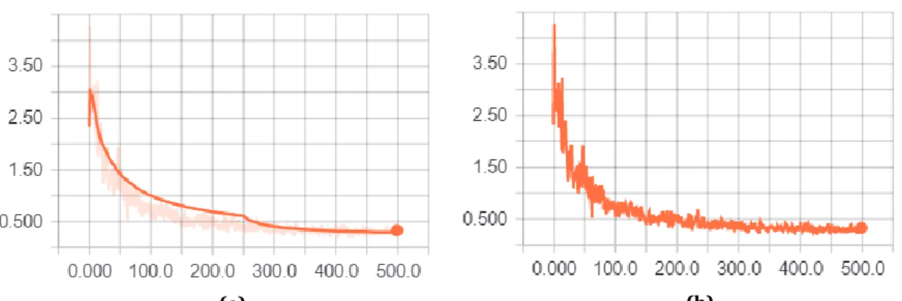
scalars, like the accuracy or the cost it is always possible to adjust the smoothing of the curve in order to understand better the real behavior of the data. Two very important parameters of the neural network are the batch size, namely how many images must be processed at every iteration and the total number of iterations. As it is shown in Figure 3-16, the number of iterations in that specific case is 500, while the used batch size is 100. These two parameters must be carefully chosen because a small batch size would need much more time to converge to a minimum, but can be more general, whereas a big batch size would behave in the opposite way. A good trade-off must be found by looking at the accuracy and the loss function that, in this case, is the cross entropy.
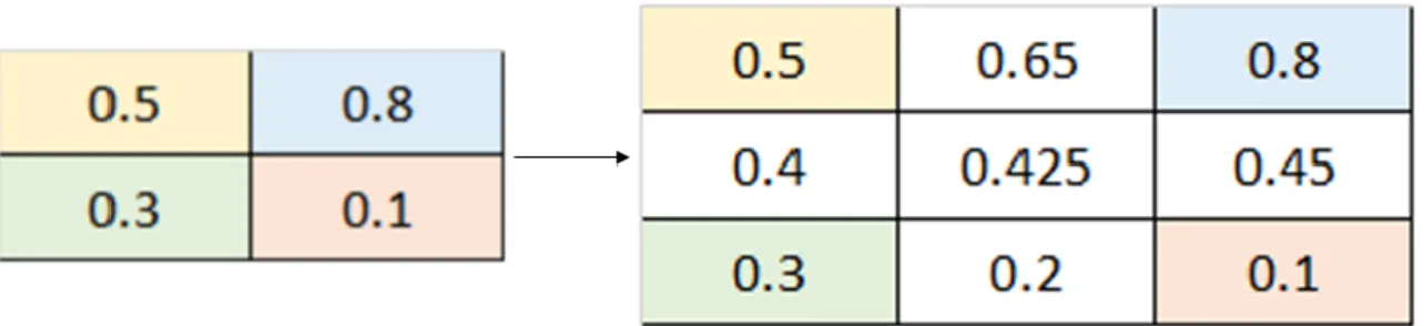
After having trained the neural network, a test dataset is created from some test images. In this case, it is not necessary to extract the patches from the test images because the convolutions of the neural network work themselves on small areas of the input images. For instance, when testing the network on the Courbevoie webcam dataset, the size of every input images is 640x471, but there is no need to modify the network. However, the changes applied to the input images by the network are the same that have been used over the training sequence and then, if the training image height is halved by the max pooling layer, the test image height will be halved as well. At the end of the pipeline, instead of a 1x1x2 tensor, i.e. two probabilities, one for each class, there will be a heat-map with a probability for every pixel of the image. The procedure to be followed is the same of the training but with trained weights and biases and different sizes:
1. Take the first image of the test dataset (in this case with size 640x471).
2. Apply 32 convolutions using a filter of size of 5x5 with the trained weights and biases; the output tensor has a size of 640x471x32. The size of every image after the convolution does not change because a padding is applied before the filter.
3. Apply the activation function.
4. Apply a max pooling with a filter of size 2x2 and a stride of 2. The output has a size of 235x320x32.