ALMA MATER STUDIORUM − UNIVERSITÀ DI BOLOGNA
CAMPUS DI CESENA
SCUOLA DI INGEGNERIA E ARCHITETTURA
Corso di Laurea Magistrale
Ingegneria Elettronica e Telecomunicazioni per l’Energia
CONTENT
CHARACTERIZATION
OF 3D VIDEOS
Tesi in:
TEORIA DELL’INFORMAZIONE LM
Tesi di Laurea di: Silvia Rossi
Relatore: Chiar.mo Prof. Marco Chiani Correlatori: Prof. Andrea Giorgetti Prof. Maria G. Martini Dott. Ing. Simone Moretti
SESSIONE III
KEY WORDS
3D Video
Depth Indicator
"...perché prima e dopo il sogno
c’è la vita da vivere."
LL
Abstract
This thesis is focused on the content characterization of Three-Dimensional (3D) videos. In a preliminary analysis, the 3D spatial and temporal com-plexity is studied following conventional techniques that are applied to Two-Dimensional (2D) videos. In particular, Spatial Information (SI) and Temporal Information (TI) are the two indicators used to describe the spatio-temporal content. To provide a complete 3D video characterization, the depth content information has to be taken into account. In this regard, four novel depth indicators are proposed based on statistical evaluations of the depth map his-togram. The first two depth indicators are based on the mean and standard deviation of the depth map data distribution. The third proposed algorithm estimates the depth of a 3D content based on the entropy of the depth map. The fourth implemented technique jointly applies a thresholding technique and analyses the residual depth map histogram calculating the Kurtosis in-dex. Several experiments are performed to validate the proposed techniques through the comparison with other objective metrics and subjective tests. The experimental results show the effectiveness of the proposed solutions to provide algorithms for the automatic depth evaluation of 3D videos. Finally, one of these new metrics is applied to a 3D video database in order to provide a real example of 3D content characterization.
Contents
Abstract vii
Introduction 1
1 3D video: State of the art 5
1.1 Brief History of 3D . . . 5
1.2 Human visual system . . . 6
1.3 3D video processing and communications . . . 8
1.4 Content generation . . . 9
1.5 3D Signal Format . . . 10
1.5.1 Stereoscopic format . . . 10
1.5.2 Video plus depth . . . 11
1.5.3 Layered depth video . . . 11
1.6 3D video compression . . . 12
1.6.1 Stereo and multiview video coding . . . 12
1.6.2 Video plus depth coding . . . 13
1.7 3D Displays . . . 14
1.7.1 Stereoscopic Display . . . 15
1.7.2 Head-Mounted Display . . . 17
1.7.3 Autostereoscopic Display . . . 18
1.7.4 Holographic Display . . . 21
2 New metrics for 3D depth characterization 23 2.1 Introduction . . . 23
2.2 Previous works: evaluation of depth perception . . . 24
2.2.1 Subjective test: depth evaluation . . . 24
2.2.2 Depth Information estimation . . . 25
2.3 Depth Map Estimation . . . 28
2.4 Proposed Depth Indicators . . . 30
2.4.2 TKDI . . . 31
2.4.3 EDI . . . 32
2.5 Performance analysis of DI . . . 33
2.5.1 Statistical Depth Indicator (DI) performance evalua-tion metrics . . . 33
2.5.2 Results . . . 35
3 Characterization of Videos 37 3.1 Introduction . . . 37
3.2 2D Videos: Spatial and Temporal Information . . . 38
3.3 Space-Time characterization of a 3D video database . . . 39
3.4 3D videos: Depth Indicator . . . 43
Conclusion 43 A Video Quality Evaluation 51 A.1 Introduction . . . 51
A.2 Subjective test methodologies . . . 51
A.2.1 Rating method . . . 52
A.3 Subjective quality test: impact of freeze frames . . . 55
A.3.1 Video selection . . . 55
A.3.2 Test section . . . 60
A.3.3 Results analysis . . . 60
List of Figures
1.1 First examples of stereoscope. . . 6
1.2 Principle of binocular vision. . . 7
1.3 Some examples of monocular cues. . . 8
1.4 3D video system . . . 9
1.5 Comparison of different stereoscopic format . . . 11
1.6 Example of Video plus depth. . . 12
1.7 Layered Depth Video (LDV). . . 12
1.8 Coding schemes for stereo and multiview video . . . 14
1.9 A hierarchy of 3D Display . . . 15
1.10 Example of image and glasses used for anaglyph technology . . 16
1.11 Polarized 3D system . . . 17
1.12 Functional principle of time multiplexed system . . . 18
1.13 Working principle of two different autostereoscopic technology 19 1.14 Multiple viewing zones produced by Autostereoscopic display 19 1.15 Multiview system [1] . . . 20
2.1 Some images from the 3D image database used for the subjec-tive tests. . . 25
2.2 Parallax calculation on 3D display. . . 26
2.3 Object detection in histogram of disparity. . . 26
2.4 a) Example of a depth map; b) The related histogram. . . 29
3.1 The video set used for the 3D analysis: Kingston videos from A to I, RMIT videos from J to M. . . 40
3.2 Spatial and temporal information for the sequences in 3D Video Database database, calculated for left and right views: Kingston videos from A to I, RMIT videos from J to M. . . . 42
3.3 Content characterization of selected 3D videos database in terms of SI and T I. . . 45
3.4 Content characterization of selected 3D videos database in terms of SI and DI. . . 46
3.5 Content characterization of selected 3D videos database in
terms of T I and DI. . . 47
3.6 Content characterization of selected 3D videos database in terms of SI, T I and DI . . . 48
A.1 Absolute Category Rating (ACR) method. . . 53
A.2 (Degradation Category Rating (DCR) method. . . 53
A.3 Pair comparison method. . . 54
A.4 Double Stimulus Continuous Quality Scale (DSCQS) method. 55 A.5 Temporal information for each selected part. In each figure, the point of rebuffering are indicated. . . 58
A.6 Frames corresponding to rebuffering positions in the video stream. . . 59
A.7 The continuous evaluation interface. . . 60
A.8 Scores of scenario 0. . . 61
A.9 Scenario 1 - Mean score difference between pattern 1 and 2 for each participant. . . 62
A.10 Scenario 2 - Mean Opinion Score sorted by number of frames and in chronological order. . . 63
List of Tables
2.1 Previous depth indicators. . . 27 2.2 Performance of selected depth indicators. The numbers are
referred to Table 2.1 . . . 36 3.1 Characteristics 3D video database: Kingston videos from A to
I, RMIT videos from J to M. The frame rate is fs=30 fps. . . 41
3.2 SI and TI values of 3D video database . . . 42 3.3 SI, TI, DI values for the video sequences of the 3D database. . 44 A.1 Duration of freeze events. . . 56 A.2 Test cases. The different colours of grey indicates each
Acronym
2D Two-Dimensional 3D Three-Dimensional 3DTV 3D TelevisionACR Absolute Category Rating
ACR-HR ACR with Hidden Reference AVC Advanced Video Coding
CSV Conventional Stereo Video DCR (Degradation Category Rating
DMAG5 Depth Map Automatic Generator 5 DMOS Differential Mean Opinion Score DI Depth Indicator
DSCQS Double Stimulus Continuous Quality Scale EPFL École polytechnique fédérale de Lausanne EDI Entropy-basedDI
FoV Field of View
FPD Flat Pannel Display fps Frame per Second H Height
HMD Head-Mounted Display HVS Human Visual System Hz Hertz
IRCCYN Institut de Recherche en Communications et Cybernétique e Nantes ITU International Telecommunications Union
LCD Liquid Crystal Display LDI Layered Depth Image LDV Layered Depth Video muDI µDIMean-basedDI MOS Mean Opinion Score MVC Multiview Video Coding MVD Multiview Video Plus Depth MVV Multiview Video
PCC Pearson Correlation Coefficient QoE Quality of Experience
RMIT3DV Royal Melbourne Institute of Technology 3DV RMSE Root Mean Square Error
RMSE* Epsilon-Insensitive RMSE RODR Regions of Depth Relevance SCC Spearman Correlation Coefficient SEI Supplemental Enhancement Information SI Spatial Information
sigmaDI σDIStandard Deviation-basedDI SS Single Stimulus
TKDI Thresholding&Kurtosis-basedDI VoD Video on Demand
Introduction
The invasion of multimedia and digital telecommunication technologies is one of the most high-impact phenomena of the modern era. Given the latest technological progress, even more evolved mobile devices appear every day on the market. The diffusion of advanced smart-phones and tablets is drasti-cally increased in the recent years. Another important step, in the technology evolution, is the wireless connectivity that is able to guarantee a fast and re-liable connection between a large number of multimedia devices. Moreover, since new mobile devices are equipped with embedded cameras, they are able to record and share video information in an easy way. In this regard, video is one of the main source of information, producing a large amount of data. In particular, recent studies report that the novel video transmission such as TV, Video on Demand (VoD), Internet, and P2P will constitute 90% of global consumer traffic by 2019 [2]. The video evolution started in the 19th
century when new techniques have been proposed for improving the quality of 2D images. Eventually, one of the most recent innovation, in the context of multimedia entertainment, is the introduction of 3D images and videos. The transition from 2D to 3D is having the same impact as the introduction of colour television in the second half of the 20thcentury [3]. The 3D technology
is devised for improving the visual quality by adding the perception of depth. It is based on the ability of the human binocular system of perceiving the tridimensionality. The human eyes capture two views of the same scene and fuse them in order to reconstruct the real depth. The stereoscopic images are the first example of 3D technique and they are based on the same principle of the human visual system. They are composed by two overlapped images that are generated with two complementary colours. In particular, special glasses, with filtering properties, have been invented to achieve image separation and perceive the sense of depth. Although the first studies on 3D dates back to 1920, this technology has become more popular only in the recent years [4]. For instance, Avatar, the first popular 3D movie, has been proposed only in 2009. Recently, 3D videos is applied to a large variety of new fields such as: entertainment (3D Television (3DTV) and 3D games), tele-medicine
(re-mote 3D surgery monitoring), education (3D tour in museum), and 3D video conference. To provide the best quality of experience for the final user, the novel 3D multimedia applications must satisfy severe requirements in terms of delay, jitter, low bit error rate during the transmission and to guarantee the best visual quality.
In this scenario, this work presents new methodologies to characterize the content of 3D videos and images. In particular, the 3D content description is provided in terms of spatial, temporal, and depth information. In the first step, 3D videos are characterized by using temporal and spatial infor-mation, applying SI and TI as in the 2D context. The main novelty of this work consists in adding the information about depth. Therefore, four novel DIs are proposed to evaluate the perceived human depth in 3D images and videos. Several experiments are performed to validate the proposed tech-niques through the comparison with other objective metrics and subjective tests. The experimental results show the effectiveness of the proposed solu-tions to provide algorithms for the automatic depth evaluation of 3D videos. Finally, one of these new metrics is applied to a 3D video database in order to provide a real example of 3D content characterization.
The remainder of this thesis is the following:
• Chapter 1 provides an overview of the state-of-the-art of the 3D tech-nologies. A brief description of the human visual system is provided in order to analyse the human perception of tridimensionality. In addi-tion, the principal 3D video acquisiaddi-tion, elaboration and visualisation techniques are studied.
• Chapter 2 proposes four novel depth indicators which are based on a statistical analysis of the depth map histogram. In particular, the two first depth indicators are based on the mean and standard deviation of the depth map data distribution. The third proposed algorithm estimates the depth based on the entropy of the depth map values. The fourth implemented technique jointly applies a thresholding technique and analyses the residual depth map distribution through the Kurtosis index. Finally, the performance of the new metrics are compared with other well-known indicators.
• Chapter 3 is focused on the content characterization of a 3D video database. In the first step, the 3D videos are characterized in terms of spatial and temporal information through SI and TI. Then, one of the implemented indicators is applied to the video database in order to provide a real example of 3D content description.
Finally, Appendix A concerns the video quality assessment. In particular, after a brief description of different subjective test methodologies, a video ob-jective quality test is reported. The purpose of this experiment consists in studying the impact of the freezing effect on the perceived quality from the final user.
The work in this thesis has been realized in the framework of a collabo-ration between University of Bologna and Kingston University in London.
Chapter 1
3D video: State of the art
1.1
Brief History of 3D
Stereoscopy, from στερεος (stereos) meaning "firm, solid" and σκοπεω (skopeo), meaning "to look, to see" is the technique for creating and displaying the il-lusion of depth in images and videos. It is based on our binocular vision system that is known since 200 b.C. as proposed by Euclid: our brain re-ceives slightly different images from eyes and is able to perceive the sense of depth (Paragraph 1.2).
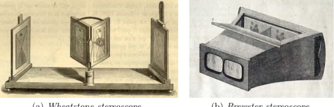
The history of stereoscopy started in 1928 with Sir Charles Wheatstone who proved that it was possible to reproduce artificially human binocular vi-sion and in 1838 designed the first stereoscope, an optical instrument based on two angled mirrors for viewing two-dimensional pictures and giving an illusion of depth. Only after the invention of photography (1839) and im-provements in technology, stereoscopy became very popular. David Brewster showed at the 1851 Great Exhibition the first stereoscopic camera and also Queen Victoria was fascinated by this new instrument. Brewster’s stereo-scopes was based on a lens system that allowed a reduction in size as showed in Figure 1.1.
With the advent of cinema, a new era of 3D reproduction began: the Lu-mière brothers in 1903 produced the first short 3D motion but only in 1922 Harry K. Fairall realised the first full-length 3D movie named "The Power of Love". It was based on anaglyph technique (Section 1.7.1): each image was coded with two different colour, red and green, and the audience was able to perceive correctly the image wearing coloured glasses. Using the same princi-ple, in 1928 John Logie Baird conducted first experiments on 3DTV. Despite these early successful demonstrations of the stereo cinema and television, the "golden era" of 3D began much later in 1952, with first colour stereoscopic
(a) Wheatstone stereoscope. (b) Brewster stereoscope.
Figure 1.1: First examples of stereoscope.
film. It was the first boom for 3D cinema and during next two years Hol-lywood produced one hundred movies in this format. However, the interest for this new technology dropped rapidly because of technical deficiencies and insufficient quality. Only the early 1990s have seen a significant revival in 3D technology due to new researches about depth perception, quality control and new technology. The movie that marked definitely the recent successful, was "Avatar" in 2009. which it has introduced this technology in our daily life [4].
1.2
Human visual system
The ability to appreciate the third dimension from the environment around us is a characteristic of our binocular visual system and is known with the term stereopsis. Because of their horizontal separation, our eyes capture slightly different images of the same object and the brain, fusing them, is able to extract the depth information. The 3D technology tries to recreate this condition to obtain the sense of depth in 2D images. Therefore this para-graph explains basic characteristics of Human Visual System (HVS) before introducing the principles of 3D technique.
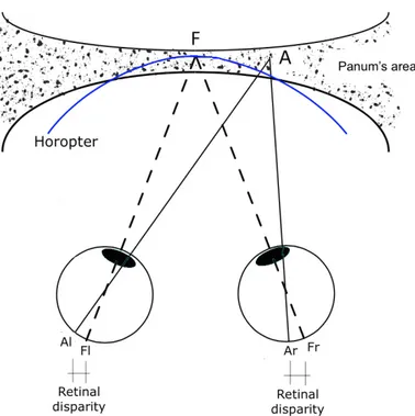
The HVS uses different cues in the process that provides the depth percep-tion and these can be divided in two groups: monocular cues and binocular cues. The latter require both eyes to perceive the depth and is more im-portant. An example of binocular cues is the retinal disparity or binocular disparity, as shown in Figure 1.2. The point F is called fixation point which when fixated is projected at the same position in both eyes and hence has zero retinal disparity. For each fixation point it is possibly define horopter: an imaginary curved line which contains all points that are at the same
ge-Figure 1.2: Principle of binocular vision.
ometrical or perceived distance of the fixation point [5]. Thus, all objects located on the horopter are beamed on the same relative coordinates in the retina of both eyes and are perceived as single images, thank to the fusion that happens in the brain. Around the horopter it is possible to define a small zone, Panum’s area, where the objects are perceived as a single one but they are projected in different position on the left and right retina. The difference between these positions is the retinal disparity.
Other examples of binocular depth cues are vergence and accommodation, two process related to each other because changes in vergence induce changes in accommodation and vice versa. First one is a mechanism by which our eyes move simultaneously in order to put the fixation object in the centre of each retina. The latter refers to the movement that optical axes do to maintain a clear vision. These cues are responsible for understanding the distance of observed objects.
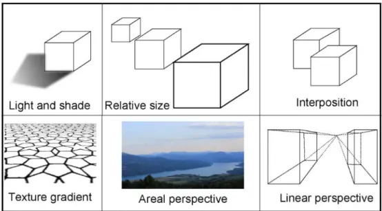
In addition to the binocular depth cues, others factors that contribute to understand depth are monocular cues which they provide depth information when viewing a scene with only one eye. Some examples are (Figure 1.3):
• light and shade: the reflected light and shadow gives information about the thickness objects in the observed scene.
Figure 1.3: Some examples of monocular cues.
• relative size: a closer object is bigger than farther one and it helps to understand their relative position.
• interposition: farther objects disappear when others overlap them and this suggest their depth order.
• texture gradient: most surfaces (e.g. walls, roads, field) have a tex-ture that appears finer and smoother with distance.
• areal perspective: contrast and colour of objects change with dis-tance due to the atmosphere.
• linear perspective: parallel lines converge and recede to the horizon.
1.3
3D video processing and communications
Today, the 3D videos have become so popular that their applications cover several varieties of environments: entertainment (3DTV, DVD, games) , medicine (3D surgery), real-time application (3D conference), education (3D picture books, 3D tour in museums), and others [6]. Irrespective of the final application, all 3D systems can be represented by the same general blocks in a end-to-end chain as shown in Figure 1.4.
In particular the chosen method of delivery is the most important com-ponent in the system because it influences other comcom-ponents. Two general
Figure 1.4: 3D video system
approaches can be used: delivery via storage on mass storage or transmission of 3D video. The latter is of more interest nowadays because it is suitable for several applications and it is possible to transmit in digital TV channels or on the Internet for HTTP streaming or VoD application.
In the following, the main steps in a 3D system, i.e. content generation, signal format, coding and displaying will be described briefly.
1.4
Content generation
The first stage in a generic 3D system is to generate the 3D content. Different type of camera systems can be used and based on the number of devices are called monoscopic systems, dual-camera systems and multi-view systems.
The monoscopic systems are very simple because it requires only one digital camera. After recording, the 2D video has to be elaborated by com-puter vision algorithms that try to extract depth information by monocular and binocular depth cues. These programs convert automatically or semi-automatically the 2D video to 3D. Hence this method is of much interest as it does not require expensive devices but with the drawback that the final quality is not always satisfying. Other example of a monoscopic system is to use a single camera in combination with other devices (e.g. laser or infra-red sensors) that records depth map which contains depth information in each pixel. Usually, these maps are stored as 8-bit image where the level 0 corre-sponds to a farther value and the level 255 coincides with a closer value [7]. Unfortunately, these devices have limited depth accuracy.
The dual-camera configuration is composed of two digital cameras posi-tioned in parallel with a horizontal separation in order to register the same scene by different point of view, basically reproducing our HVS. The main drawback in this approach are synchronization and camera calibration. It is possible to adjust the image pairs post-production but it is limited and time consuming. An approach to overcome these problems is to use 3D state-of-the-art cameras that record one conventional video combined with a depth map. One of the latest version of this type of cameras, for example, capture a High Definition (HD) colour picture and calculate the depth using a
succes-sion of short light pulses transmitted in the direction of the scene. The depth in fact is inversely proportional to the energy of the light that comes back when it collides with an object. This approach allows a easy post producing but the cameras are usually very expensive.
The multi-view systems is an array of more than two monoscopic cam-eras. Hence the results are more precise but calibration and synchronization problems are inherent to these systems.
1.5
3D Signal Format
There are different formats for acquiring 3D videos; however, 3D video format capable to serve a wide range of 3D applications are the most efficient [8].
1.5.1
Stereoscopic format
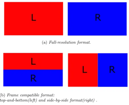
The Conventional Stereo Video (CSV) or stereoscopic 3D video signal is the most well-known and simple format: it is developed to be used with existing technologies, such as coding/decoding system for 2D videos. In it turn, stereoscopic format can be divided in two types: full resolution video or frame compatible format as shown in Figure 1.5.
Full resolution video is composed by two distinct 2D videos with full resolution, one is for the left eye and the other one for the right eye. The two streams can be elaborated as typical 2D videos separately but, in this way, the amount generated data is double compared to the 2D video.
The frame compatible format tries to solve this problem with the two stereo views multiplexed in a single frame. Spatial multiplexing techniques can be applied: each view has half horizontal (side-by-side) or half vertical resolution (top-bottom). Temporal multiplexing is also possible: the frames of two views are saved sequentially with full spatial resolution. In both cases, the amount of data is the same as of a single view since the total resolution of the two views is equal to a single 2D image. A Temporal multiplexing extension is the Multiview Video (MVV). It is composed by multiple views of the same scene but captured from different points. It has been devised for advanced 3D video application, e.g. multiview autostereoscopic displays and free viewpoint videos (see 1.7). Obviously, the amount of data for this format increases significantly.
(a) Full-resolution format.
(b) Frame compatible format:
top-and-bottom(left) and side-by-side format(right) .
Figure 1.5: Comparison of different stereoscopic format
1.5.2
Video plus depth
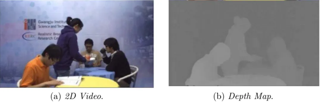
Another format is the video plus depth which is a regular 2D video with a depth map. An example is shown in Figure 1.6. The depth map represents the depth information or more precisely the distance from the camera to each point in the filmed scene. It can be considered a monochromatic luminance signal with a restricted range between [Znear, Zf ar]. The 2D video gives
in-formation about the structure of the scene and colour intensity.
Video plus depth format is really efficient due to the backward compatibility and extended functionality that allows to adjusted the 3D perception before visualization. On the other hand, it is difficult to generate an accurate depth map.
Also in this representation, it has been proposed the related extension (namely Multiview Video Plus Depth (MVD)) that is able to give higher accuracy re-spect to the previous formats.
1.5.3
Layered depth video
A Layered Depth Video (LDV) is a an extension of the Layered Depth Image (LDI)format as proposed since 1998 [9]. As shown in Figure 1.7, this format is composed by a 2D colour image with its depth map as in the previous
(a) 2D Video. (b) Depth Map.
Figure 1.6: Example of Video plus depth.
format, and a background layer with associated depth map. The latter layer includes only image content which is covered by objects in the main layer while the rest is omitted [10]. Thus, LDV might be more efficient than MVD because is able to produce lower data rates.
Figure 1.7: Layered Depth Video (LDV).
1.6
3D video compression
Several 3D video coding techniques have been designed. In this section we briefly discuss some of the states of the art technique based on the 3D video formats discussed in previous section [11].
1.6.1
Stereo and multiview video coding
H.264/MPEG4-AVC
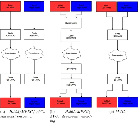
The first example of video coding for stereoscopic 3D video is H.264/MPEG4-Advanced Video Coding (AVC) that can be used with a frame-compatible coding scheme.
• Simulcast encoding (Figure 1.8 (a)): each view is encoded and trans-mitted independently and is not synchronized. It is very simple and compatible with most of the standard video coders but has reduced compression capability because it does not take into account the infor-mation of redundancy between the two views.
• Dependent encoding (Figure 1.8 (b)): each picture contains both the views that are packed either "side-by-side" or "top-and-bottom". Prior to display, the views are required to be sampled to the appropriate resolution. In order to guarantee that the decoder is able to distinguish the left and right view inside the multiplexed stream, the standard expects a Supplemental Enhancement Information (SEI) message. Multiview video coding (MVC)
An important extension of H.264/MPEG4-AVC, it is Multiview Video Cod-ing (MVC) which was standardized in 2009. It codes efficiently stereo and multiview video [12]. This solution takes advantage of not only temporal re-dundancies between the frames in one view but also the similarities between neighbouring frames (Figure 1.8 (c)). It allows also partial decoding of a single view thus providing backward compatibility with old systems.
1.6.2
Video plus depth coding
The simplest approach to encode video plus depth is coding independently both 2D video and depth map using H.264/AVC. However, it has the same drawbacks of synchronization and low compression as that of simulcast en-coding in H.264/MPEG4.
MPEG-C Part 3
For optimized compression of the 3D format, a new standardized format MPEG-C Part 3 has been proposed recently. It allows encoding the 3D con-tent as conventional 2D sequence with additional parameters for interpreting the decoded depth values at the receiver side. Especially it is compatible with any existing deployment of H.264/AVC because the used video codec for both colour video and depth video signal is H.264/AVC. Moreover, Eu-ropean projects have shown that for a encoded depth map with good quality it is sufficient only 10%-20% of the bit rate used for the colour video [13]. Thus, this format is interesting from compression efficiency point of views thanks to the characteristics of the depth data.
(a) H.264/MPEG4-AVC: simulcast encoding.
(b) H.264/MPEG4-AVC: dependent encod-ing.
(c) MVC.
Figure 1.8: Coding schemes for stereo and multiview video
1.7
3D Displays
The last but not the least step in a 3D video system is the 3D display, a device capable to give the perception of depth in the visualized video. A common characteristic is that it requires at least two views of the same scene captured from different perspectives in order to recreate our HVS (see Paragraph 1.2). In this section an overview of the state-of-the-art technologies in 3D display with their advantages and disadvantages are discussed.
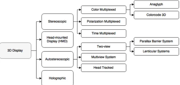
There are different methods of classification but in this work the technolo-gies currently being used are divided into the following categories: Stereo-scopic Display, Auto-stereoStereo-scopic Display, Head-Mounted Display, Holographic Display [14]. Figure 1.9 shows this classification.
Figure 1.9: A hierarchy of 3D Display
1.7.1
Stereoscopic Display
The stereoscopic technology was the first display technology ever used to give the sensation of depth on a 2D screen. The main requirement of stereoscopic videos or images is to capture the same scene from two different positions and it is needed that the two views are presented separately so each eyes see only one views. This requirement of eye separation is achieved by means of special glasses that the viewer wears while viewing the stereoscopic image. There are different ways to obtain the image separation: using different colours, polarization or time multiplexed. In the first two cases the glasses include no active electronic elements and are therefore termed "passive". In the last one it is required that the glasses are synchronized with the display, so they are called "active".
Colour Multiplexed Approach
Anaglyph technique is an example of separation by colour: the left and right images are generated with a couple of complementary colours. These images are showed in the same time on the screen but, thanks to the glasses each eye is able to see only one view per time. The most common colour filter used is red for the left eye and cyan for the right. In figure 1.10 is shown an example of anaglyph image and glasses used as filter.
This method can be used in any device capable of reproducing colour (elec-tronic devices but also paper) and it is an inexpensive solution, thanks to easy-to-manufacture glasses. Due to the quality limits of the filters, images
for one eye sometimes gets mixed with the other eye’s images, a problem commonly known as crosstalk. Furthermore, the images are of full colour-resolution but each eye receives them as non-full-colour because of the glasses that block a specific colour. Another drawback is that the brightness of im-ages for each eye may vary and so the eye watching darker frames feels dull, an effect known as flicker effect.
(a) Anaglyph of Saguaro National Park at dusk 3D red cyan glasses are recommended to view this image correctly. [15] .
(b) Color-coded anaglyph glass.
Figure 1.10: Example of image and glasses used for anaglyph technology An evolution of anaglyph images is the ColorCode 3D. It was deployed in the 2000s and produces full-colour 3D images which are viewed with amber and blue colour glassed. ColorCode 3D, like all stereoscopic 3D technologies, reduces the overall brightness of the viewed image and also can cause ghosting images.
Polarization-Multiplexed Approach
In one of the most common current technology, each image is polarized. An optical filter is used that allows light beams of a specific polarization angle to pass and blocks light beams of other angles. Each image is showed at the same time but their polarization is made mutually orthogonal in order to have the image separation. The viewer wears eye-wear with appropriate polarization to block the image not intended for that eye. It is also possible to use linear or circular polarization. With linear polarization the position of the viewer’s head needs to have a precise location to perceive 3D vision. With circular polarization this constraint is no more necessary. Even if the
polarization solution solves several drawbacks (e.g. no-full-colour resolution and flicker effect), it is more expensive and complex because demands a new type of screen in order to preserve the state of polarization.
(a) Functional principle of polarized 3D tech-nology. [15] .
(b) Polarized glass.
Figure 1.11: Polarized 3D system
Time-Multiplexed Approach
The solutions explained until here are based on spatial multiplexing. In this new approach, instead, the left and right images are not shown at the same time but are displayed on the screen in alternating fashion at high frame rate, usually 120 Hertz (Hz). In this case the viewer has to wear a pair of active shutter glasses, which are synchronized to the content being displayed on the screen. The active glasses are controlled by an infra-red signal sent from the television and when the left-eye image is shown, they block reception of the right eye and vice versa. This approach provides the best 3D performance compared to other stereoscopic techniques because it assures full-colour as well as full-resolution images. However, an immediate disadvantage is the cost of the active shutter glasses and software required for synchronization system. Furthermore there does not exist a standardised infra-red signal for this technology. Thus, eyeglasses of one particular display may not work with another one and it could give rise to interference problems.
1.7.2
Head-Mounted Display
A Head-Mounted Display (HMD) is a display system that can provide the viewer with a sense of immersion in a displayed scene since the device is worn on the head. It consists of two displays which show directly the left and right images to the respective eye. Nowadays such systems are widely used for training purposes in the medical, military and industrial fields. However, it
Figure 1.12: Functional principle of time multiplexed system
is not easy to provide a large Field of View (FoV) and high resolution at the same time.
1.7.3
Autostereoscopic Display
Autostereoscopic display provides the binocular perception of 3D without requiring any special glasses. This technology is used on Liquid Crystal Display (LCD) since they offer good pixel position tolerance and can be successfully combined with different optical elements. The main limitations of this technology is the cost and number of users able to perceive depth at the same time.
In the following section are discuss two different types of autostereoscopic display: two-view and multiple display.
Two-view autostereoscopic Display
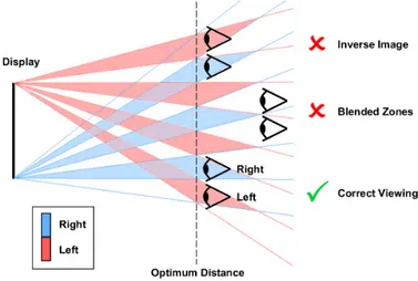
Two-view display are the older and simpler autostereoscopic display. In this technology only one stereo image is displayed at the same time and so there is a limited area where the viewer’s eyes have to be to perceive correctly the depth. There are two different working principle: parallax barrier and lenticular lenses. The first, as show in Figure 1.13(a), requires a barrier in front of the screen. Left and right image are both shown but placed alternately in column and the parallax barrier, which is composed of vertical apertures separated by black masks allowing light to pass only toward the desired eye. The parallax barrier can be turned on/off electronically in order to have a system 2D/3D switchable system. This approach produces multiple viewing zones (Figure 1.14). Only when the viewer is standing at the ideal distance and in the correct position, he/she is able to perceive the depth sensation. For this reason the viewer has 50% chance to be in the wrong
(a) Parallax Barrier (b) Lenticular Screen
Figure 1.13: Working principle of two different autostereoscopic technology position and see an incorrect image [1]. The optimum viewing distance is proportional to the space between the display and the parallax barrier and is inversely proportional to the display pixel size. Other disadvantage of these kind of 3D display is the loss of spatial resolution because only half display is available overall for each eye. There is also loss of brightness caused by the barriers.
Figure 1.14: Multiple viewing zones produced by Autostereoscopic display Figure 1.13(b) shows the lenticular system. It is composed of a Flat Pannel Display (FPD) with cylindrical lenses that direct the light from a pixel towards a specific direction and each column of pixels is visible only from a particular zone around to the display. Similar to parallax barrier system, only when the viewer is in a right position, 3D perception is satisfied.
It is also possible have a 2D/3D switchable system using special lenses that can be change electronically between refracting (3D) and non-refracting (2D) modes. Anyway there is a residual lens effect that last even if the display is working in the 2D way. The disadvantages caused by multiple viewing zones are present in this approach as well.
Multiview Autostereoscopic Display
A multiview system provides the viewing of multiple pairs of stereoscopic im-ages. The main advantage is that the viewer is able to perceive a 3D image anywhere inside the viewing zone as shown in Figure 1.15(a).
The main disadvantage of multiview displays is the difficulty of building a display that is able to show at the same time multiple views of the same image.
(a) Viewing zone (b) Multi-projector system
Figure 1.15: Multiview system [1]
Parallax barrier and lenticular screen, discussed before, can be applied to obtain a multiview autostereoscopic display. Multi-projector is another ap-proach: each view requests a single projector that project on a special screen (Figure 1.15 (b)). Because of the high number of projectors, this method is expensive and requires that the images are aligned precisely.
Head Tracked Display
An other kind of autostereoscopic system is the head tracked display that try to adjust the viewing zone according to viewer’s head or eye position. This display may reduce the discomfort for the viewer but requires state-of-the-art technology to track the right position.
There are several head tracking methods such as electromechanical, electro-magnetic, acoustic and optical tracking [16]. It is highly important to guar-antee that the position is accurately tracked and the scene updates very fast
in accordance to viewers’ movement. Thus some advanced systems combine many of these different methods to make the tracker more robust.
1.7.4
Holographic Display
Unlike stereoscopic technology that is based on our depth perception, holo-graphic display allows a comfortable viewing experience because it is able to recreate an object in three physical dimensions. It is a technique known since 1948 but several obstacles have prevented this technology from becom-ing popular and only recently these have been addressed [17].
The basic principle of holographic is to record the space with all its phys-ical properties and then generate a light field that represent optphys-ically the scene. Unfortunately, huge amount of information is required to generate holograms. In order to overcome this problem, there are different strategies such as eye-tracking that is able to generate holographic images only in a narrow region that the viewer sees.
Volumetric displays are an evolution of this technique. They are screen com-posed by voxels, e.g. pixels in a 3D grid that represent an object in a space [18].
Chapter 2
New metrics for 3D depth
characterization
2.1
Introduction
One of the most important metric to evaluate the efficiency and the reliabil-ity of modern video communication and processing techniques is the Qualreliabil-ity of Experience (QoE). The QoE has been introduced in [19] as the over-all acceptability of an application or service, as perceived subjectively by the end-user; following the mentioned definition, QoE is a quality indicator which is fundamentally based on the final point of view. Successively, other QoE definition have been proposed. For example, in [20] the QoE is defined as the degree of delight or annoyance of the user of an application or service. It results from the fulfillment of the expectations with respect to the utility and/or enjoyment of the application or service in the light of the user’s per-sonality. When a novel technology implies the video transmission, one of the most reliable way to evaluate the QoE is the subjective tests. Nowadays, 3D video entertainment is one of the most attractive and promising field for sci-entific research and innovative video applications. Considering this aspect, there is a need to provide efficient systems for a realiable QoE evaluation for the novel 3D technologies [21]. While 2D video assessment has been a widely studied field, the 3D video quality evaluation has need of be investi-gated more. As mentioned in 3.2, SI and TI are two indicators capable to describe the complexity of 2D images. These parameters, however, provide only a measurement of spatial and temporal complexity and do not provide information on the depth content of an image or video sequence. Therefore, it is necessary to find new techniques to describe the contents of 3D images and videos. A 3D video is jointly composed of two 2D videos and the related
information on the depth of the filmed scene. Considering this aspect, it is reasonable to use the SI and TI indicators for studying the temporal and spatial complexity of the two 2D views. However, a new metric is required to additionally take into account the depth.
In this Chapter, four novel Depth Indicators (DIs) for 3D videos are presented which are based on the study of the histogram of the depth map greyvalues. The aim of these indicator is that to estimate with objective values, the per-ceived depth by human observers. Initially, an overview of previous works found in literature is provided. In particular, several works concerning the depth estimation and the software used for calculating the depth map are studied. In the second phase, the four proposed DIs are described. To eval-uate the reliability of the proposed techniques, the DIs are compared with other well-known metrics.
2.2
Previous works:
evaluation of depth perception
In literature, several depth estimation algorithms for 3D images are pre-sented. In particular, 31 different DI algorithms have been studied and im-plemented [22]. The main idea consists of comparing these 31 algorithms with the 3 novel proposed DI techniques. Since the final objective is to iden-tify a depth index that represents the human perception of depth, several subjective tests have been performed to evaluate the perceived depth of sev-eral 3D images. These subjective tests are used as metric reference to analyse the performances of the implemented DIs.
2.2.1
Subjective test: depth evaluation
In [22], subjective tests are performed in order to test the efficiency of the DI algorithm. Twenty users rated 200 images about the personal perceived depth [22]. The Absolute Category Rating ACR (as described in A.2.1) is used for evaluating the subjective test results. The rated images belongs to a public image database that has been developed with the aim to investigate the contribution of monocular and binocular depth cues in natural images [23]. These images present a variety of depth properties (e.g. linear perspective, texture gradient, relative size and defocus blur). Figure 2.1 shows some examples of the used images.
(a) (b) (c)
(d) (e) (f)
Figure 2.1: Some images from the 3D image database used for the subjective tests.
2.2.2
Depth Information estimation
As described in 1.2, the disparity is one of the major factors that influence the binocular vision. Therefore, the studied metrics are mainly based on the disparity between left and right view. They can be divided into three categories: distance, volume and object-based metrics [24].
In the first group, 19 of the 31 studied metrics corresponding to 1-19 in Ta-ble 2.1 are based on statistical data analysis: the depth is measured referring to a particular value of percentile (from 0.05% to 99.5%) of disparity values in the depth map.
The volume metrics evaluate the whole distribution of disparity values. Three of the considered volume metrics (20-22 in Table 2.1) are based on the differ-ence between two of the previously considered percentile values. The metric 23 in Table 2.1 calculates the standard deviation of the distance metrics [24]. In its turn, metric 24 is based on the luminance contrast as proposed in [24]. The last considered volume metric (25 in Table 2.1) calculates the depth per-ception as a function of average parallax and range parallax [25]. Parallax is the difference between the object’s position shown on a 3D display and its apparent position (Figure 2.2) as defined by the equation:
P = β − α. (2.1)
Finally, five object-based metrics, capable of evaluating the depth based on the object decomposition, are studied (27-31 in Table 2.1). The metric 27 in Table 2.1 counts the detected objects corresponding to the peaks in the
Figure 2.2: Parallax calculation on 3D display.
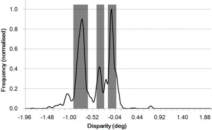
histogram of Figure 2.3. The metric 28 computes the difference between the farthest and nearest detected objects. In its turn, the metric 29 in Table 2.1 computes the object thickness. In Figure 2.3, the rectangle width represents the computed thickness.
The metric 30 in Table 2.1 is one of the most complex object metrics: the
Figure 2.3: Object detection in histogram of disparity.
objects are detected thanks to the segmentation maps [26]. In particular, only the Regions of Depth Relevance (RODR) are selected for estimating the depth. The metric 31 Table 2.1 is jointly based on the disparity values and the width of the objects that are detected through the segmentation map [27].
Nr. METRICS Distance metrics 1 P005 2 P010 3 P015 4 P020 5 P025 6 P050 7 P075 8 P100 9 P125 10 P500 11 P875 12 P900 13 P925 14 P950 15 P975 16 P980 17 P985 18 P990 19 P995 V olume metrics 20 P950-P050 21 P975-P025 22 P990-P010 23 Standard Deviation 24 Michelson contrast
25 2nd order polynomial fit [25]
26 2nd order polynomial refit [25]
Ob
j.
metric
27 Avg. Thickness
28 Depth Interval btw Objects
29 Number Objects
30 PerceptualDepthIndicator [26]
31 Object thickness [27]
2.3
Depth Map Estimation
All the mentioned algorithms are based on disparity values. Therefore, an accurate depth map estimation is needed. In [22], a well known optical flow based algorithm is used [28]. However, the depth map estimation tool in [28] is not able to compute the depth map for some particular images (dark images and images with a predominant color). Due to this reason, other tools have been searched and the Depth Map Automatic Generator 5 (DMAG5) [29] has been selected for this work. The implementation of this algorithm is proposed in [30]. The selected algorithm estimates the depth map of stereo images taking the left view as the reference and the right as target. The depth estimation is achieved considering the position difference of each pixel between the reference and the target image. Recent studies have demonstrated that label-based approaches can be successfully applied to many computer vision task such as stereo matching problems. For instance the chosen label could be the disparity in order to evaluate the depth map. The main drawback of these approaches is the high computational time. Therefore, the aim of authors in [30] consists of proposing a filter-based algorithm for general multi-labelling problems able to evaluate the disparity map in real time mode. This approach is based on three main steps:
• Definition of a cost-volume function that assigns a cost for the chosen label at all pixel in the image.
• Filtering the cost-volume using a guided filter which is able to preserve edges. The guided filter is a moving average filter.
• Labeling selection looking for the value that minimizes the cost associ-ated to every pixel, i.e. Winner-take-all strategy [31].
Some parameters are required to obtain a correct depth map. The input parameters are listed and described below.
• Minimum Disparity is the difference between the position of the fur-thest point in the images left and right.
• Maximum Disparity is the difference between the position of the closest point in the images left and right.
• Window Radius is the filter size that calculates the disparity between the images.
• Alpha balances the colour and the gradient matching cost. The closer is alpha to 0, the more important is the considered colour.
• Truncation Value - colour limits the color value. • Truncation Value - gradient limits the gradient value. • Epsilon controls the smoothness of the depth map.
• Nbr of smoothing iterations indicates how many times the disparities pixels are smoothed.
A detailed analysis about the influence of these parameters on the disparity estimation is proposed in [31]. Although the best value for each parameter depends on the image type, some parameters can be generically setted. For example, better results are obtained with large values of windows radius, color and gradient truncation. The influence of alpha depends on texture of the scene, e.g. for higher textured images the disparity evaluation is better with high values of this parameter. Figure 2.4(a) depicts the depth map evaluated for the image 2.1(a) and the associated histogram in (b).
(a)
(b)
2.4
Proposed Depth Indicators
In the context of the 3D video characterisation, four novel depth indicators have been proposed. For each depth of them, the histogram of the depth map has been analysed. An histogram is a graphical representation of the distribution of numerical data. In the context of 3D images, the histogram of the depth map provides some information about the object distribution within the 3D images. Considering a n bit grey level depth map, the related histogram is composed by a discrete and integer number of bins [0, L-1] where L = 2n. Each bin defines the number of pixel (frequency) in the depth map, that have the related gray value. In particular, lower bin values correspond to object that are placed in proximity of the camera while, higher values refers to objects that are far away from the camera.
The histogram of a digital image of size M × N with grey levels in the range [0, L-1] is a discrete function:
h(rk) = fk (2.2)
where
• rk is the kth grey level (depth),
• fk is the number of pixels in the image having gray level rk,
• h(rk)is the histogram of a M × N digital image with grey levels rk.
Based on the analysis of the histogram, four depth indicators are pre-sented. The first algorithm, namely Standard Deviation-basedDI (σDI), is based on the statistical analysis of the depth map histogram. The second proposed algorithm, denoted as Thresholding&Kurtosis-basedDI (TKDI), jointly applies a thresholding technique (usually used in the 2D images) and a statistical indicator capable to estimate the similarity between the depth histogram distribution and a Gaussian one. Finally, Entropy-basedDI (EDI) is proposed to estimate the depth of an image based on the study of the histogram entropy.
In the following, the proposed metrics of this work are presented in detail.
2.4.1
µDI, σDI
As a first simple metric we propose the mean value of the depth map as a possible indicator, defined as:
µDI =
L−1
X
k=0
where:
• pk = M ·Nfk is the normalized histogram value.
Analysing the histograms over a wide set of 3D images, it is noticed that very deep images are characterized by histograms with a predominant mean value and decreasing distribution around this value. These peaks depict predominant objects in the scene. These are the parts in the views more extended at the same distance. Therefore, from the observer point of view, the presence of these objects is important for the perception of depth; they are taken as reference as cues of depth. Following the previous observation, σDI estimates the depth calculating the standard deviation of the depth map distribution. This DI statistically measures the data dispersion respect to the mean value. In particular, low standard deviation values mean that the data set tends to be very close to the mean value, while high values indicate that the data are largely spread in a certain range.
Given the histogram of a depth map defined as in (2.2), the σDI is defined as: σDI = v u u t L−1 X k=0 pk· (rk− µDI)2. (2.4)
2.4.2
TKDI
The analysis of the deep image histograms reveals a correlation between the depth of images and the distribution of their histograms. Therefore, the second proposed algorithm, denoted as TKDI is based on the estimation of the Gaussianity of the depth histograms. Before this statistical analysis, the depth histogram is processed with a thresholding technique. In the 2D world, thresholding is a technique able to separate the background and the foreground of an image. In TKDI, the depth histogram is thresholded in order to analyse only the histogram values that provides a real contribution to the depth estimation. In particular, Otsu’s technique is applied [32]. The principle of this algorithm is that a 2D image contains two groups of pixel forming the foreground and background part. The optimum threshold is calculated in order to divide the two classes of pixels. In particular, the threshold is chosen in order maximize the inter-class variance of the pixel. Given the histogram of depth map defined as in Equation (2.2), the Otsu’s algorithm looks for a threshold T following these main steps:
2. Look up n1(T ) = |fk≤ T |, n2(T ) = |fk > T | in the histogram and
calculate both cluster means.
3. Compute the weighted within-class variance as: σ2(T ) = n1(T ) · n2(T ) (M · N )2 · [µ1(T ) − µ2(T )] 2 where • µ1(T ) = σ1/n2(T ). • µ2(T ) = σ2/n1(T ).
• σ1 and σ2 are the variances of cluster 1 and 2.
Finally, the optimum threshold is chosen as: T∗ = arg max
T [σ 2(T )].
In the second phase, the residual histogram is analysed calculating the Kur-tosis index which measures the level of tailless of the probability distribution of a random variable. Therefore, the Kurtosis index is calculated with the residual values as:
TKDI = µ4(fk) σ4(f k) = E[fk− ¯f ] 4 (E[(fk− ¯f )2])2 . (2.5)
2.4.3
EDI
The last proposed metric, namely EDI, is based on the computation of the entropy of the depth map data distribution. In general the entropy is a indicator of the uncertainty of the information contained in a data distribu-tion. Taking into account this condition, very deep image are characterized by high value of entropy. Given the histogram of depth map defined as in Equation (2.2), EDI is defined as:
EDI = −
L−1
X
k=0
2.5
Performance analysis of DI
The performance between of each proposed DI and the 31 algorithms de-scribed in 2.2.2 are compared in the following. Since each depth indicator has a proper scale, a third order polynomial function is applied in order to uniform the different metrics scales and the Mean Opinion Score (MOS) value obtained through the subjective tests.
2.5.1
Statistical DI performance evaluation metrics
Four evaluation metrics are implemented in order to compare each DI with the results provided by the subjective test in [33]. In particular, Pearson Correlation Coefficient (PCC) evaluates the linear correlation between two sets of data. The Root Mean Square Error (RMSE) of the Pe is the second
evaluation metric and it measures the accuracy between two data sets. In addition, a third statistical indicator is provided and it is denoted as Epsilon-Insensitive RMSE (RMSE*). This metric is a RMSE modified version and it additionally takes in account the uncertainty on the analysed data. Finally, Spearman Correlation Coefficient (SCC) measures the statistical dependence between two variables.
Pearson Correlation Coefficient (PCC)
The PCC is used to measure the linear correlation between two data sets. Given two data sets, α and β, composed by N elements, it is defined:
• αi as the value of the ithelements in α (in this work, αi is the MOS for
the ith image).
• βi as the value of the ith elements in β (in this work, βi is the DI value
for the ith image of one of the implemented depth indicators).
Based on the previous definitions, PCC computes the linear correlation as follows: P CC(α, β) = N X i=1 (αi− α) · (βi− β) v u u t N X i=1 (αi− α)2· v u u t N X i=1 (βi − β)2 (2.7)
where: • α = 1 N N X i=1 αi and β = 1 N N X i=1 βi. RMSE
This metric evaluates the accuracy of the objective metric.
Defined α and β as in PCC, the prediction error Prediction Error (Pe) for
each sample is:
Pe(i) = αi− βi. (2.8)
To compute Pe it is required that α and β have the same scale. This is
obtained by applying an interpolation with a third-degree polynomial func-tion as described in the introducfunc-tion of this secfunc-tion. Therefore, the RMSE is calculated as: RM SE = v u u t 1 N − 1 N X i=1 Pe(i)2. (2.9) RMSE*
Epsilon-Insensitive RMSE (RMSE*) is a RMSE modified version and it takes into account the 95% confidence interval of the MOS values.
In RMSE*, the Pe for each single value is defined as:
Pe∗(i) = max(0, |αi− βi| − ci95). (2.10)
where ci95 is the 95% confidence interval of the averaged α and it is
deter-mined using the t-Student distribution. Finally, the RMSE* is defined as:
RM SE∗ = v u u t 1 N − d N X i=1 P∗ e(i)2. (2.11) where:
• d the number of freedom (d=4 if a 3th order mapping function is used
Spearman Correlation Coefficient (SCC)
Differently to the other considered metrics, SCC is based on the ranking of the two data distribution. Specifically, the two data sets are sorted in ascending order based on the MOS value and each considered DI.
Defined:
• R(αi) as the ranking position of the MOS of the ith image,
• R(βi) as the ranking position of the ith image considering one of the
implemented DI, the SCC is calculated as:
SCC = 1 − 6 N X i=1 (R(αi) − R(βi))2 N3− N . (2.12)
2.5.2
Results
In this section, the comparison of µDI, TKDI and EDI is performed over the 3D image database described in 2.2.1. In particular, the DIs are calculated over a specific image subset. The database in [22] is composed by 200 images; however only 45 images have been chosen in this work. The selected subset is composed by natural images with no acquisition artifacts (e.g. the blurring effect) and post-acquisition elaborations (e.g. resizing). This selection has been performed to eliminate any further influencing factors in judging the image depth during the subjective tests. Successively, the MOS values, for the selected images, are obtained from [22].
The performance of the all DIs have been evaluated through the statistical coefficients described in 2.5.1. For the sake of simplicity, the proposed DIs are compared with 3 of the 31 indicators (see 2.2.2) which provide the best performance. In particular, metric 7, 26, and 30 (see Table 2.1 ) are selected. In Table 2.2, the evaluated DIs are compared with the results provided by the subjective tests. Through the presented results, the correlation between objective and subjective tests is studied: taking the subjective results as metric reference, the higher is the correlation with the subjective tests the more efficient is the considered DI. Therefore, the higher is the PCC and SCC values, the better are the DI performance. Conversely, low RMSE and RMSE* values correspond to a better capability in the depth estimation. Considering the PCC values, from Table 2.2, all the proposed metrics obtain the best results: specifically, the DI based on the entropy evaluation (EDI)
Nr METRICS PCC SCC RMSE RMSE*
7 P075 0.511 0.576 3.900 3.105
26 2nd order polynomial refit [25] 0.532 0.558 3.882 3.070
30 PerceptualDepthIndicator [26] 0.494 0.525 3.874 3.060
32 µDI 0.608 0.429 3.239 2.472
33 TKDI 0.601 0.530 3.263 2.529
34 EDI 0.679 0.567 3.279 2.524
Table 2.2: Performance of selected depth indicators. The numbers are re-ferred to Table 2.1
achieves the highest PCC value. Otherwise, metric 7 is the best DI if the SCC values are taken into account. It is worth noticing that this metric it is not well-defined since it depends on the considered percentile value (see Table 2.1) and it is strictly related to the considered image set. In conclusion, the results in Table 2.2 prove that the proposed metrics are characterized by a higher level of reliability respect to the metrics present in literature.
Chapter 3
Characterization of Videos
3.1
Introduction
The information extraction from a video sequence is a challenging task to be pursued in order to perform efficient video characterization and classification. In this regard, several works are present in literature in which the video characterization is based on technical parameters or content information [34]. However, the major part of the proposed works are related to 2D videos: due to the increased adoption of 3D videos in the recent years, similar approach are studied to perform smart video characterization in the 3D context. For instance, this characterization could be a way to describe the complexity of 3D videos and could be used in the selection of source for subjective video quality assessment. As described in Chapter 1, a 3D stereoscopic video is basically composed by two 2D videos. Therefore, one of the possible approach is to describe spatial and temporal complexity with the same indicators used for a typical 2D content. However, for an effective 3D video characterization a fundamental information must be additionally taken into account: the depth. One of the main objectives of this thesis is to characterize a 3D video database based on specific content video information. The objective is to provide a video classification reference for future experiments.
In this Chapter, the indicators used to characterize spatial and temporal complexity in a 2D video are described and applied to a 3D database video as initial step in the content characterization. Finally, one of the implemented indicators is applied to the video database in order to provide a real example of 3D content description.
3.2
2D Videos: Spatial and Temporal
Information
Subjective video quality tests are a fundamental tool for the QoE evalu-ation in the video/image processing context. A reliable perceived quality analysis entails an appropriate video sequence selection. The use of video se-quences characterized by different quality (e.g. motion, level of details, type of scene) leverages an accurate QoE analysis. Therefore, these sequences should be chosen in order to cover a large set of characteristics. In par-ticular, spatial and temporal data are efficient indicators to determine the relation between achievable video compression and the final perceived qual-ity. Recommendation ITU-T P.910 [35] defines Spatial Information (SI) and Temporal Information (TI) as objective metrics to quantify the spatial and temporal perceptual information. Furthermore, [35] recommends the em-ploying of a video set capable to cover the whole spatio-temporal plan. SI and TI indicators are based on the luminance plane and they characterize the quality of each video frame by a single value.
SI measures the amount of spatial details in a frame [35]. The principle is the following: the higher is the number of high-contrast areas in a frame, the larger is the presence of edges, and the more relevant is the spatial infor-mation. Given a video sequence with a MxN image size, SI is based on the application of the Sobel filter on the luminance matrix (Fn) of the
consid-ered nth frame in order to identify horizontal and vertical edges. The Sobel
function is defined as follow:
Yn = Sobel(Fn) (3.1)
where Yn is the matrix that identifies the related edges by the Sobel filter.
Defined Yn(i, j) as the generic elements of Yn, where i and j are the ith row
and jth column, SI for the nth frame is computed as the standard deviation
in the following way: SIn= v u u t 1 (M − 1)(N − 1) N X i=1 M X j=1 (Yn(i, j) − Yn)2 (3.2)
where Yn is the Yn mean value and is calculated as:
Yn = 1 M N N X i=1 M X j=1 Yn(i, j).
In its turn, TI measures the amount of temporal variations in a video sequence [35]; high TI values correspond to high quantity of movement. It-eratively, TI calculates the temporal variation between two adjacent frame performing a pixel-to-pixel comparison, as:
Mn(i, j) = Fn(i, j) − Fn−1(i, j) (3.3)
where Fnis luminance matrix, and i and j are the ith row and jth column of
nth frame.
Based on (3.3), TI computes the standard deviation over the whole pixel differance set, in the following way:
T In= v u u t 1 (M − 1)(N − 1) N X i=1 M X j=1 (Mn(i, j) − Mn)2 (3.4)
where Mn is the mean value defined as:
Mn= 1 M N N X i=1 M X j=1 Mn(i, j).
Typically, TI and SI are employed for the video content information and classification. In [35], a proposed approach consists of taking the maximum value over the whole considered video as defined in bellow:
SI = max n SIn (3.5) T I = max n T In. (3.6)
3.3
Space-Time characterization of a
3D video database
In the first step of this characterization work, a 3D video database of the Kingston University, London [36] has been analysed to achieve a 3D content characterization in terms of spatial and temporal information. This database, freely accessible for scientific research purposes, is composed by nine stereo-scopic videos: for each video the left and right views are available. Figure 3.1 (A)-(I) shows a frame from each of the nine videos. In Table 3.1-left, the resolution and the number of frames for each video sequence are provided.
(A) Lovebird 1 (B) Newspaper (C) Kendo
(D) Beergarden (E) Cafe (F) Ballroom
(G) Mobile (H) Horse (I) Car
(J) Skateboard (K) Bike (L) Motorway
(M) Library
Figure 3.1: The video set used for the 3D analysis: Kingston videos from A to I, RMIT videos from J to M.
Videos Resolutions N. Frames A - Lovebird 1 1024x768 300 B - Newspaper 1024x768 300 C - Kendo 1024x768 300 D - Beergarden 1920x1080 150 E - Cafe 1920x1080 300 F - Ballroom 640x480 250 G - Mobile 720x540 200 H - Horse 480x270 140 I - Car 480x270 235 J - Skateboard 1920x1080 250 K - Bike 1920x1080 300 L - Motorway 1920x1080 300 M - Library 1920x1080 298
Table 3.1: Characteristics 3D video database: Kingston videos from A to I, RMIT videos from J to M. The frame rate is fs=30 fps.
In Table 3.2, the SI and TI values for the both views of the considered videos are provided. As it can be noticed from Figure 3.2, the Kingston video database does not entirely span the SI-TI range as request. To cover the spatio-temporal domain in a more homogeneous way, other available 3D videos database have been analysed.
There are few examples of public 3D video database; in this work, other three database are analysed in terms of SI and TI. For example, six 3D videos are available from the École polytechnique fédérale de Lausanne (EPFL)-Switzerland [37]. These sequences last 10 seconds and the employed cameras are placed at different distances from the scene. A second database composed by ten stereoscopic videos is presented by the Institut de Recherche en Com-munications et Cybernétique e Nantes (IRCCYN) in order to investigate dif-ferent research areas in 3D technology, such as subjective assessment, depth estimation, objective quality metrics, and visual discomfort [38]. Finally, the Royal Melbourne Institute of Technology 3DV (RMIT3DV) database is composed by 31 uncompressed HD 3D [39].
The SI and TI values are calculated for all the mentioned database and four videos, from RMIT3DV database, have been chosen in order to have a more distributed SI-TI range values. In particular, the selected videos are char-acterized by variable camera position or high quantity of movement that guarantee high TI values. In Figure 3.1 J-M, one frame from each selected video is shown and technical information are reported in the right Table 3.2.
Kingston Database SI TI Video A right 60.851 11.007left 62.803 11.850 Video B right 67.76left 64.57 15.0115.29 Video C right 59.43left 57.98 23.4323.75 Video D right 83.57left 83.73 13.1113.88 Video E right 56.33left 56.95 12.5012.46 Video F right 77.08left 77.14 26.7326.96 Video G right 96.52left 93.20 14.9115.40 Video H right 74.73left 77.96 19.3218.77 Video I right 56.32left 54.99 13.8214.50
RMIT Database SI TI Video J right 69.61 28.66left 59.35 26.98 Video K right 83.41 31.66left 77.90 30.38 Video L right 89.95 24.21left 88.76 23.90 Video M right 81.06 25.99left 87.19 26.90
Table 3.2: SI and TI values of 3D video database
50 55 60 65 70 75 80 85 90 95 100 10 15 20 25 30
Spatial Information (SI)
Temporal Information (TI)
Video A Video B Video C Video D Video E Video F Video G Video H Video I Video J Video K Video L Video M
Figure 3.2: Spatial and temporal information for the sequences in 3D Video Database database, calculated for left and right views: Kingston videos from A to I, RMIT videos from J to M.