A digital approach for the automatic definition of performance evaluation models for flow-/job-shops

(1)

Scuola di Ingegneria Industriale e dell’Informazione

Master’s Degree in Management Engineering

Master’s Degree Thesis

A digital approach for the automatic

definition of performance evaluation

models for flow-/job-shops

Supervisor

Prof. Marcello URGO

Doc. Massimo MANZINI

Candidate

Filippo BORTOLOTTI

Student number

905363

(2)

The increasing request of connectivity and interoperability in the manufacturing sector, in particular for small and middle size companies, creates the need of flexible and integrated solutions for the management and performance evaluation of a system.

The objective of this thesis is to define an approach for the representation of a physical production system and from it developing a procedure for the automatic generation of performance evaluation models. The approach aims to represent an ontology based production system in a queuing network trough the definition of modelling hypothesis and rules. Next step is to apply the model to integrate the ontology production system to the simulation tool for the performance evaluation. This integration is possible by analysing both the connected elements to understand how the data can be extracted from the ontology and how the approximate model can be imported in the simulation tool. This approach is then verified through the definition of multiple study case where for each of them, some approximate model KPIs are compared with the one obtained from a commercial software. Moreover, a possible representation of assembly system for the performance evaluation tool has been presented and validated.

(3)

L’aumento della richiesta di connecttività e interoperabilità all’interno del settore industriale crea la necessità di ottenere soluzioni integrate e flessibili per la gestione e la misurazione delle performance per un sistema produttivo.

L’obiettivo della tesi è quello di definire un approccio per la rappresentazione di un sistema produttivo fisico e da esso sviluppare una procedura per la generazione automatica di modelli per la valutazione delle performance. L’approccio mira a rappresentare un sistema produttivo basato sull’ontologia con un sistema di code attraverso la definizione di regole e ipotesi di modellizzazione. Il prossimo passo è quello di applicare il modello per intrgrare il sistema produttivo di ontologia al tool di simulazione per la valutazione delle performance.

Questa integrazione è possible analizzando entrambi gli elementi connessi e capendo come i dati possano essere estratti dall’ontologia e come il modello approssimato possa essere importato nel tool di simulazione. Questo approccio è poi verificato attraverso la definizione di multipli case study dove per ognuno di essi alcuni KPI del modello approssimato sono confrontati con quelli ottenuti da un software commerciale. In più, una possibile rappresentazione di un sistema di assemblaggio per il tool di valutazione delle performance viene presentata e validata

(4)

(5)

List of Tables v

List of Figures vi

1 Introduction 1

2 State of the art ₄

2.1 Digital system representation . . . 5

2.2 Performance evaluation . . . 7

2.3 Automatic generation of a performance evaluation model . . . 8

3 Problem Statement 10 3.1 Analysis of the production system . . . 14

3.2 Analysis of the buffer . . . 15

3.3 Analysis of the relationship between . . . 17

4 Solution 19 4.1 JMT JSIM Formalization . . . 20

4.1.1 Station definition . . . 20

4.1.1.1 Queue . . . 20

4.1.1.2 Source and Sink . . . 22

4.1.2 Class Definition . . . 22

4.1.3 Performance Evaluation . . . 23

4.2 Data extraction from ontology . . . 24

4.2.1 Ontology preparation . . . 24

4.2.2 Queries definition . . . 25

4.2.2.1 Physical system stations . . . 27

4.2.2.2 Buffer Size . . . 28

4.2.2.3 Part Types . . . 29

4.2.2.4 Process Steps . . . 30

(6)

4.2.4 Data Refinement . . . 37

4.2.4.1 Physical system stations . . . 37

4.2.4.2 Buffer size . . . 38

4.2.4.3 Part types . . . 38

4.2.4.4 Process steps . . . 38

4.2.4.5 Assignment of processes steps to machines . . . 39

4.2.4.6 Assignment of stocastic processes steps to machines 39 4.2.4.7 Part type flow . . . 39

4.2.4.8 Buffer and machine merging . . . 40

4.2.4.9 Arrival time and number of population . . . 40

4.3 XML Modelling . . . 40 4.3.1 Heading . . . 44 4.3.2 Source . . . 45 4.3.3 Queue station . . . 47 4.3.4 Sink . . . 51 4.3.5 Connections . . . 51 4.3.6 Performance to be evaluated . . . 52

4.3.7 Load of population for closed system . . . 53

4.3.8 Ending . . . 53

4.4 Run Simulation . . . 53

4.4.1 JMT JSIM user interface approach . . . 54

4.4.2 Console simulation run . . . 55

4.5 Output Reading and Results Analysis . . . 56

5 Validation of the model ₅₉ 5.1 Flow shop . . . 61

5.1.1 Flow Shop single class . . . 61

5.1.2 Flow Shop multi class . . . 63

5.2 Hybrid flow shop . . . 64

5.2.1 Hybrid flow shop single class . . . 64

5.2.2 Hybrid flow Shop multi class . . . 66

5.3 Job shop . . . 68

5.4 Real Industrial case . . . 69

5.4.1 JMT JSIM representation . . . 72

6 Conclusion 77

A XML generation 79

(7)

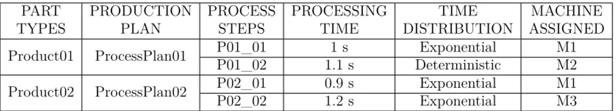
4.1 process plan for SPARQL extraction case study . . . 37

5.1 Process plan flow shop case study . . . 61

5.2 Hypothesis test results for flow shop single class . . . 62

5.3 Hypothesis test results for flow shop single class in blocking situation 62 5.4 Hypothesis test results for flow shop multi class . . . 64

5.5 Process plan hybrid flow shop study . . . 65

5.6 Hypothesis test results for hybrid flow shop single class . . . 66

5.7 Hypothesis test results for hybrid flow shop multi class . . . 67

5.8 process plan job shop case study . . . 68

5.9 hypothesis test results on job shop production system . . . 69

5.10 processing time of assembly system . . . 71

(8)

2.1 OntoGui user interface example . . . 6

2.2 Hierarchy of Ontology Modules . . . 7

2.3 Example of a system representation in JMT JSIM user interface . . 8

2.4 Scheme representing JMT JSIM XML structure . . . 9

3.1 OntoGui ontology structure . . . 11

3.2 JMT JSIM representation open hybrid flow shop single class . . . . 12

3.3 Ontology structure for system definition . . . 13

3.4 Example for a queuing network with the server . . . 13

4.1 Solution summary . . . 19

4.2 scheme representing the data extraction process. . . 24

4.3 Hierarchy of Ontology Modules . . . 26

4.4 SPARQL query case study system representation . . . 37

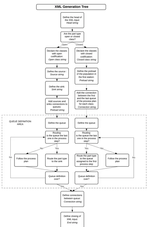
4.5 XML generation process . . . 43

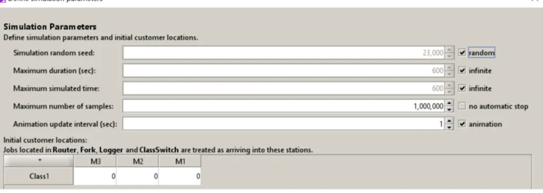
4.6 JMT JSIM simulation parameter . . . 54

5.1 Flow shop physical system . . . 61

5.2 Plant Simulation representation flow shop single class . . . 62

5.3 Plant Simulation representation flow shop multi class . . . 64

5.4 Hybrid flow shop physical system . . . 65

5.5 Hybrid flow shop Plant Simulation system . . . 65

5.6 Plant Simulation hybrid flow shop multi class system representation 66 5.7 Jobshop system representation . . . 68

5.8 Plant Simulation Jobshop system representation . . . 69

5.9 representation of the assemble hinge . . . 70

5.10 Model of an assembly line similar to the case study one . . . 70

5.11 cosberg assembly line representation . . . 72

5.12 Fork and Join component structure . . . 73

5.13 JMT JSIM representation of Industrial case study . . . 74

(9)

(10)

Introduction

Nowadays, the digital world is acquiring more and more importance. With the new revolution of Industry 4.0, also manufacturing industry is showing signs of this shift to the connected environment. The manufacturing industry shows trend towards automation and data exchange in manufacturing technologies and processes such as cyber-physical systems, the internet of things devices and cloud computing. These solutions can be achieved with an interconnected system, where data are immediately available and updated; grounding on this, a new need of connection solutions arises.

In particular, manufacturing sector experienced a shift to a continuous improvement focus exploiting new technologies available on the market. Under this light, also the production plan design requires solution for the improvement of the efficiency. During the life cycle of a production system, there could be multiple events that trigger the change or reconfiguration of the system. Every time the system changes is it needed to define a new formal representation, a new model of this system and the performance analysis representation. This performance analysis can be conducted with an analytical approach or through a simulation by exploiting different techniques and obtaining results with a different level of detail. The focus of this thesis is on the simulation side. The process of updating a system can require multiple step in order to find the best solution. During each step, the physical model is defined with the new parameters, then the simulation model is created based on the physical one and the simulation is launched. The performance are collected and evaluated by comparing the data with the previous one and the process can start again. A search of the most suitable solution requires multiple analysis, and for each analysis, multiple update of the system according to the different representation, such as physical and simulation model.

In the market, there are available simulation tools which let the user define a single system keeping the formal and performance evaluation representation connected. The problem is that these software are expensive, which limit their use,

(11)

and have a rigid structure that allows only a little integration with external tools. In the design and configuration phase, multiple systems, have to be evaluated in order to obtain the best solution. In this evaluation phase, there are lot of other elements to be considered together with production KPIs, such as physical location of the production system, CAPEX and OPEX; these parameters to include in the choice are scattered along different tools. The lack of integration of the commercial software requires a manual update of every single representation. A definition of an automatic tools for the generation and performance estimation of a system could improve the efficiency of this process. The objective of the thesis is to define a model for the representation of a physical production system from a ontology representation to a queuing network representation and, based on that, to develop a tool for the conduct of automatic performance evaluation without the need of a manual update.

This solution is possible through the use of open-source tools in order to obtain the maximum possible flexibility. For this reason, we focus on the use of ontology representation. The use of an ontology-based representation in the manufacturing environment is increasing in the lasts years thanks to open standards which allow the creation of connections between system [1]. The use of an ontology allows us to formally represent the production system and use this representation as a way to integrate different software coming from different ICT companies, including performance evaluation tools.

The first barrier to the diffused use of ontology is an efficient instantiation and management tool [2]. For this reason, OntoGui software can be adopted to overcome this obstacle and define the production system with simplicity through the use of its GUI.

Regarding the choice of the simulation tool, we consider the use of Java Modelling Tool (JMT from now on), a free open source suite. The suite uses an XML data layer that enables full re-usability of the computational engines. It consists of six tools, such as SimWiz (Java Simulation Textual) , JSIM Graph (Java Simulation Graphic), JMVA (Java Mean Value Analysis), JMCH (Java Markov Chain), JABA (Asymptotic Bound Analysis) and JVAT (Java Workload Analyzer Tool ). In particular, we will consider the use of JMT JSIM that allows exact and approximate analysis of single-class or multi-class product-form queuing networks, processing open, closed or mixed workloads.

With this availability of tools whose flexibility allows a high level of iteroperability, there is the need to understand how to create this connection. After the definition of the model from the ontology structure to the queuing network representation, the focus of the research is moved to develop a bridge between the system represented in the ontology for the performance evaluation process. We will work on the definition on this connection using the OntoGui for the ontology representation and JMT JSIM as the performance evaluation tool.

(12)

The results of this thesis will be part of the results of EU funded project called VLFT: Virtual Leaning Factory Toolkit [3]. The aim of VLFT convey the results of research activities in the field of digital manufacturing, starting from modelling, performance evaluation and virtual and augmented reality into the curriculum of engineering students. The final objective of this project is to use these virtual tools to support the students in learning complex engineering concepts and enhance their learning ability. The project consortium is composed of three different uni-versities in Europe: Politecnico di Milano, Tallinna Tehnikaulikool and Chalmers Tekniska Högskola, and two research centers: STIIMA-CNR and MTA-SZTAKI. VLFT project is supported and funded from ERASMUS +, for this reason they are defined also activities in collaboration with foreign students and workshop in project partner premises.

The project also includes the definition of a case study grounding on a real produc-tion system. The industrial partner is Cosberg, an italian manufacturing company located in Bergamo area. Cosberg design and create machines and modules for the automation of assembling processes. One of their new assembly line is used as the case study to be developed. This case study will be used for the application and testing for the generation tool developed.

In Chapter 2, one it is defined is is defined the state of the art si discussed, where it is also explained the use of the tools used. In Chapter 3, it is described the creation of the model requiring the analysis of both the element of the connection in order to define hypotheses and rules for the a valid approximation. Chapter 4 discusses how the data defined necessary for the model definition can be obtained from the ontology and how its model representation has to be encoded to define the system in JMT JSIM for the performance evaluation. This step requires the understanding of the OntoGui structure and the XML standard input required by the simulation software.

Chapter 5 involves the real performance evaluation and its verification to prove the model ability to approximate the original system.

Final consideration of the possibilities and the limits of the model, and possible future improvement are defined in Chapter 6 .

(13)

State of the art

In this chapter is being analysed the context in which this thesis is being developed and what is the current research in the topic defined. In the first part it is introduced the new connection need that is increasing in the industry. In Section (2.1 it is defined what are the possible solution for the digital representation of a system. Section 2.2 discusses about the performance evaluation issue and what is the solution chosen.

The thesis lies in the new industrial revolution called Industry 4.0 . This new revolution brings with itself a new definition of system: there are not more small systems with a limited way to communicate with each others, but everything is connected. Each system should be able to exchange data with others without any limitation. In particular, the manufacturing sector shows a great interest in this change, due to the presence of multiple sub system within a single system: the physical production line, its digital representation on various tools, the sensors able to collect data from the line and the KPIs obtained. The different sub-system representation are all independent, for this reason any update on the real system requires the change to be manually defined on each of its representation. This updating process can be addressed by the creation of connections between the different representations that a change in one of it can also be applied simultaneously to the linked systems. Due to the increase of digital tools in the industry, the need of interoperability is more and more critical.

The market already provided some solutions with professional digital tools which includes "all in one" solutions to include different type of representations of the system. These software can answer to the need of the manufacturing sector but present some limitations. For example, the interoperability of the various system representations is defined only within the tool boundaries, connections from it to an external one is limited or even not possible. Moreover, these solutions can be too expensive for small and middle players in the industry forcing them to rely on

(14)

different and scattered solutions. In particular, they have to rely on various tools for the representation of physical production system and their performance evaluation. For this reason a change of even a single parameter in the physical system requires the need to update of the simulation model. During a system creation or update the number of times that a system has to be changed are countless, each parameters has its effect on the system, thus, the possibilities to analyse are wide; a lack of connection is only decreasing the efficiency of the whole process. This issue will be analysed in detail in this chapter.

Research on the topic has been conducted over the years looking for a way to create an open system representation which could grant connections with other digital tools where data are defined in different structures. In particular for the performance evaluation field this has been deeply studied.

In this problem there are two element to analyse before the definition of a connec-tion model: the system representaconnec-tion and the performance evaluaconnec-tion.

2.1 Digital system representation

The digital system representation is the key structure of the whole process since all tools refer to this definition for their execution. Due to its central position, it is crucial to find a structure that allows the integration of fragmented data models into a unique model without losing the notation and style of the individual ones. An effective data model has to include information in relation to both the physical production system and the intangible representation given by the products and their production plans. Different solutions can be found in the existing documentation. [1].

For example, consider the ANSI/ISA-95 [4], which is is an international standard for the development of interfaces. This standard proves to be effective to represent processing and production system but has some limits regarding integration with physical representation tools.

Another solution can be found with the Process Specification Language (PSL) standard [5]. PSL standard is an ontology-based standard which allows a robust representation of a process and its characteristic together with a good level of interoperability.

A valuables standard to consider is The Industry Foundation Classes (IFC) standard by buildingSMART [6] which provides most of the definitions needed to represent tangible elements of a manufacturing systems and it is possible to include also the intangible ones through definitions provided. The connection capability of the PSL standard is given from the ontology-based structure. An ontology encloses the representation and the definition of categories, properties and connections between

(15)

entities defined in a single or multiple system. Their open definition allows the integration without the risk of losing level of details of the data such as the notation [7].

One of the most common languages for an ontology definition is OWL, Web Ontology Language, it is a semantic web language designed for ontology representation. The benefit given from an ontology-based system are countermeasured by a difficulty instantiation of the OWL ontology which limit their use to the general public. A solution to this issue is proposed through the use of OntoGui [2]. OntoGui is a tool presenting a Graphical User Interface for Rapid Instantiation of OWL Ontologies. The tool allows the definition of both physical production system and product process plan through a user interface which deeply simplify the process. It can be possible to see the user interface in Figure 2.1 .

Figure 2.1: OntoGui user interface example

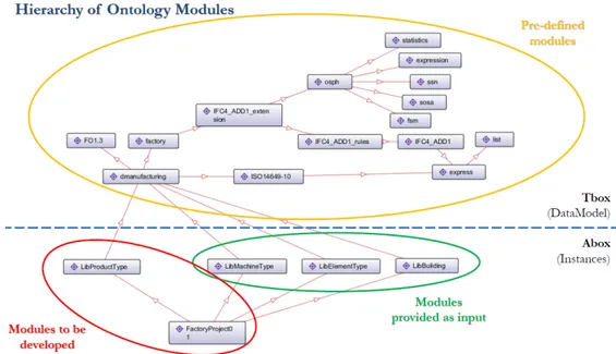
OntoGui is defined by different modules, some of them are pre-defined, while others provided as input or to be developed. The hierarchy of the ontology modules is depicted in Figure 4.3.

(16)

Figure 2.2: Hierarchy of Ontology Modules

2.2 Performance evaluation

Once the system representation has been identified, it is needed to analyse the second element of the connection model: the performance evaluation.

The choice of design for a manufacturing system comes from the evaluation of their performance in the production process [1]. For this evaluation two main approaches can be used:

• Analytical model: using mathematical or symbolic relationships to provide a formal description of the system

• Simulation models: designing a dynamic model of an actual dynamic system for the purpose either of understanding the behavior of the system or of evaluating various strategies (within the limits imposed by a criterion or set of criteria) for the operation of the system.

Analytical model proves faster results but with more approximation while simulation one can provide a higher level of precision but it is a slower process, moreover, this high level can only be reached from a really formal and wide definition of the original production system.

A lot of simulation commercial tools are available on the market but most of them lack of the connectivity capabilities needed. Moreover, the objective is to rely on open source software that can be accessible from a wider audience. We consider the use of JMT [8] tool. This tool is an open source software developed from

(17)

Politecnico di Milano and Imperial College London based on Java language. It provides six different tools performance evaluation, capacity planning, workload characterization, and modelling of computer and communication systems. The one used for the simulation is JMT JSIM which allows the discrete-event simulation for the analysis of queuing network and Petri net models through a intuitive user-interface; it can be possible to see an example in Figure 2.3. The simulation is based in queuing network which is a really important feature to the future definition of the model.

JMT JSIM is particularly interesting since it works through a XML layer to

Figure 2.3: Example of a system representation in JMT JSIM user interface connect the model definition to the analytical and simulation engine, a scheme can be found in Figure 2.4. In fact the system to be analysed can be defined through the GUI or through an XML format input. The second method allows the possibility of integration with the ontology by defining an appropriate XML based on the ontology model created.The great diffusion of this markup language makes the integration easier.

2.3 Automatic generation of a performance

eval-uation model

Once the tools used have been defined, it is needed how to understand how automatically generate the simulation model which can be represent the ontology

(18)

Figure 2.4: Scheme representing JMT JSIM XML structure

system.

The challenge of modelling is to define a general workflow to be applied for different systems but able to represent them correctly. All the steps for the definition of models and its application have been studied and defined at the end of the previous century [9]. The model has to be created with clear hypothesis and rules defining its field of application.

The new challenge is to define the connection between the system representation and the performance evaluation. Connection between an ontology based system and an JMT JSIM XML codification is not been defined yet. On the other side, there are tools for the extraction of data from the ontology exploiting SPARQL queries. For this reason a coding phase is required to create the connection once the data are obtained.

With this analysis concluded it can be possible to move to the problem statement phase of chapter 3, where all the hypothesis and rules of the modelling are defined according to the knowledge collected in this chapter.

(19)

Problem Statement

In this chapter it defined the model for the system representation. This model grounds on a set of rules and hypothesis that are defined by an analysis on the problem presented in Chapter 1.

The chapter is organized as follow: analysis of the problem and identification of the issues that requires modelling hypotheses, production system issue analysis (Section 3.1), buffer issue analysis (Section 3.2) and buffer and machine relationship

analysis (Section 3.3).

The starting point of the modelling is the structure that defines the data rep-resentation in the tools used for the physical system reprep-resentation and for the performance evaluation.

A production system in order to be suitable for this model has to respect the following assumptions:

1. It must represent a flow shop, hybrid flow shop or a job shop;

2. All machines assigned to each process step can be visited with the right sequence from the part types, thus, the production plan has to be feasible with respect to the physical system;

3. each machine has a dedicated buffer;

4. The product of a process plan strictly follow the flow defined, there are no split, for example reworking.

OntoGui product and physical representadio present an ontology-based formal-ization which can be find represented in Figure 3.1 [10]. In particular, the modules represent:

(20)

Figure 3.1: OntoGui ontology structure

• IfcTypeProcess: Definition of specific process plans; • IfcProcess: Definition of specific production process steps;

• IfcProduct: Definition of factory elements like Buffer elements, Machine tools, Pallets;

• IfcGroup: Definition of transformation systems;

• IfcControl: Definition of a work plan (e.g. production plan) to control the behaviour of a system.

From this structure, which can also be defined as process-based, the physical system and the products are defined separately. The reason of this formalization can be found in the high interoperability that it grants. This tree structure allows the data to be integrated but on the same way to maintain their original representation.

On the other side JMT JSIM adopt a flow based formalization which results in a merge between the process plan with the physical system. This structure is easier for an user to be understood and applied but limits the possible exchange of data with other tools. This difference between the two formalizations makes necessary the process of create a model to move from one to another. The differences requires definition of hypotheses and rules to limit and approximate the system that can be represented from the model.

It is needed to start from the idea that is at the base of the different representations. From one side there is the ontology, a way to create flexible data model by integrating various knowledge domains without loss for any individual one. On the other side there is a queuing network structure with a very limited flexibility, also due to the presence of a user interface with increase the restrictions. This difference can be seen by looking at the data representation of ontology from Figure 3.1 and the structure of queuing network in Figure 3.2

Before continuing it is important to understand how the the creation of a production system is defined in OntoGui. This step will help the reader to have a clear idea on the following steps, please refers to Figure 2.1 for a view on the user

(21)

Figure 3.2: JMT JSIM representation open hybrid flow shop single class

interface. The definition part can be defined into two parts, the first one defines the creation of a library for the production plan, while in the second defines the creation of a subfolder, where the previous library is imported, where the physical system is designed and the process steps can be assigned to the physical machine.

A complete production plan definition is composed into three main steps: the part type is created, a process plan assigned to the part is created, process steps of the plan are defined and for each of them it is defined the order and the processing time. In order to define the physical system the subfolder has to be created and the previous library imported; at this point it is possible to define each buffer and machine element in the system with their parameter such as buffer size, and define the physical connection. Last step is to assign each process step to the machine needed in order to define the connection between the physical system and the process plans. For this reason, what really connects the product and the physical machines is the assignment of a precise machine, or multiple ones in case of parallel processing, to a process step of a determined process plan to produce/assemble a part type. This representation of a product defines the ontology as process plan based.

Thus, the real link between the two entities, physical system and production plan, is the machine assigned to the process step. As it is discussed later this definition is critical and must always be considered during the modelling process. The concept expressed in the previous lines is depicted in Figure 3.3, where the ramification clearly shows the two part of the ontology connecting trough the machine assignment. Excluding that point, there is no other connection, thus, due to this logic, the buffer has no product assignment.

This representation has a great impact on the modelling that will be developed in the following steps, needing the creation of precise rules and hypothesis on the representation of the buffers. Moving to the queuing network, before going into detail it is important to focus its main characteristic. A queuing system is defined by one or more “customers” waiting for a service by one or more ”servers”. Queue forms due to a not perfect balance between the arrival rate of the customers

(22)

Figure 3.3: Ontology structure for system definition

and the service rate of the service. An example can be found in Figure 3.4 A

Figure 3.4: Example for a queuing network with the server

queuing network has different characteristic in the analysis: the number of the population, the arrival process, the service process, the queue configuration and the queue discipline. For some of these parameters there is the need to create some assumption which are defined along the chapter.

Due to this different structure, process plan is assigned differently to the physical system. The user must define the “class” which represent the products, and the physical production system. At this point the assignment of the production/assem-bly processes to the machines is direct, there is no process plan to define.

As explained in Chapter 2, in this kind of network each station is composed in 3 main parts: the queue section, the service section and the routing section. The first one is responsible for the buffer of the station, the second one to the processing time and the last one to the direction that each product is taking after leaving the station. For this reason, the definition of the physical system is merged with the one of each part type and its process plan.

The addition of the process step characteristic within a station parameter represents a critical change compared to the Ontology definition. There is a merging of information that in the original representation are kept separated and finds the only point of contact through the assignment of the machine to a single process step. In this way, a queuing network eliminates the need of defining a

(23)

process plan separately. This define that the new representation necessary for the performance evaluation is Flow Based which simply means that for each product it is necessary to define all the machine visited with their processing time and set the routing of the part types from machine to machine.

The new radical change is the basis of the modelling of the new system. The first objective is to understand what needs to be limited passing from an open and flexible model to a strict one. Following this which information are necessary to operate from production plan based to flow based system.

3.1 Analysis of the production system

In this section, the first problem related to the difference between a flow-based logic and a production plan logic is analysed. The two different data structures have a different system definition and it is needed to find an approach to pass from first to the second.It has been seen how the two different codification change the system definition. In a practical way, moving from the first to the second means starting from a product with its production plan and obtain a list of all the machines visited from the product. Doing this for all the part type of the system completes the process.

These two different approaches also change the way to define the type of pro-duction system. Let us start from the hypothesis that all the part type defined in the same ontology library are assigned to the same physical system and there it is not possible to define the system without one of them. With this approximation, a production system is composed of: part types and their process plan and a physical system where the process steps are assigned to. There can’t be any process step that is not assigned to an existing machine. System with more flexibility such as open shop can be easily distinguished from more rigid one such as flow shop, due to the presence of multiple following process steps. For other cases, without the definition of the production system it can’t be possible to operate this distinction. For example, a flow shop and a job shop from only the point of view of the process plan cannot be defined, it is its assignment on physical machines that creates the type definition. On the other side in the queuing network the physical system defined together with the process steps, so there is no space for flexibility. These is no possibility to assign the process steps of a “class” to another system.

Moreover, system with less constraints, such as open shop, grants higher flexibility but this flexibility requires a wider analysis of the ontology structure. For this reason, in order to start the analysis with more focus, it has been defined another hypothesis which limits the field of application of the model: only systems that can be included under the categories of flow shop, hybrid flow shop (flow shop with

(24)

parallel machines) and job shop without parallel machines are considered. Opening the definition to more complex system would increase greatly the definition of the model. Once the model is defined it can be possible to go back and remove some constraints and start again a new analysis.

Another issue that need to be faced in before continuing with the in-depth analysis of the XML input file, regards the buffers station of the physical system.

3.2 Analysis of the buffer

This problem comes from the different concept of buffer between the Ontology defined structure and the queuing network. In OntoGui the buffer is an independent element of the production system, completely separated from the machines, on the other way in queuing network there is no real representation of the buffer. The buffer is represented as the queue section inside a station. Within the same station, as wrote before, there is both the queue and the service section, where the last one represents the machine in the Ontology. This duality of a station creates a great issue to be solved.

Going back to the concept of production plan and flow-based representation, it’s critical to understand how the buffer issue can be faced in these two different models. Starting from the ontology, the part types are connected to the physical system through the process steps which have the machines assigned; on the other side there is no real direct connection with the buffers. It is no possible to act on the linking between a buffer and a product. This relationship can be easily deduced in case of simpler production system such as flow shop; in fact in relation to the this system, if a buffer is connected downstream a machine and upstream another, and both of them are visited in succession from a certain part type, this means that also the buffer is being crossed from the same product. In cases where there is more than one buffer between two machines, it is not feasible to claim that the path of the part types crosses the buffer.

This lack of information is a cause of great uncertainty which need to eliminate for the fact that the model to be developed is going to be applied from a program, which is not able to reason like a human mind in case of ambiguous situation like this one. First of all there is to consider that the model is already limited to production system such as: flow shop, hybrid flow shop and job shop which are already limiting the variety of buffer configuration.

Starting from this point it is important also to point out again that the ontology is not containing any information on how buffers are being assigned to products. For this reason, even if it was possible to convert with any change the production system it would still be a certain level of lack of data for a correct and reliable

(25)

performance evaluation. Due to this issue, it is easier to have a new hypothesis that there is only one buffer before each machine, this solution is also going to become handy in following problems. This new rule can look like a limitation but considering the constraints we already have and the lack of parameters in the ontology, it has a limited impact, with great improvement in term of performance evaluation and on the reliability of the model within its hypothesis.

The definition of a single, machine-dedicated buffer puts a limit in the use of this model to already defined ontology production system. This approach let the user define its own approximation so that the results can be as closest as possible to its own point of view in the buffer management.

Within a buffer station there are various possible strategies that can be imple-mented. The first one is the queue policy, so how products in queue should behave while waiting in the buffer. It can be defined into two levels, a general station level and a part type level. For the station specific level, it represents the general queue policy without distinction between classes of product. For this policy the best general approach is the non-pre-emptive scheduling for all the queue element. It grants a better modelling for the production system considered in the hypothesis already made.

Going to focus on the single part type it can be possible to define a queue policy also for the single product. Due to the lack of this definition in the ontologies taken into analysis and the need of simplify the initial model, it is decided that the best option is to use for all buffer a FCFS logic. The policies chosen represent the most common type for the production system analysis, so these hypotheses still grant the most general approach as possible in terms of queue policies.

Another parameter to analyse is the “drop rule”, so how each station should behave with the products within it when there is a blocking situation in the system. It is important to define this parameter since it has a great effect on the system performance. Discarding a product other than keep it waiting in the queue until the next one has space again can have multiple impact such as on throughput and time spent in the system. Considering the kind of system it is being modelled, it can be easily excluded a rule based on dropping the product out of the system such as it could be modelled a real person queue for a service provided. The logic to follow is to be able to represent at the best the majority as possible of the production system that respect the boundaries expressed by the hypothesis. For this reason, the best rule to apply would be the block after service one. In this way, the part types that have just finished their operation in a station must wait in the service station until the end of blocking if they find the buffer of the following station full.

After a definition of the main hypothesis for the buffer part of a station there is the need also to define some rules for the processing. In the ontology, it is possible to define a wider set of processing rules thank to the fact of the great versatility of the structure, on the other side from the queuing network the regulation can be

(26)

more imiting. The machines are considered to process only one product per time, so each process step has 100% usage on each station, considering a processing time which is always load independent and that can be defined only trough deterministic or exponential distribution. The last hypothesis is simply defined in order to develop a model that is able to consider more than one time distribution, so a being able to recognise the kind of input, but to keep easier the creation of it.

3.3 Analysis of the relationship between

The last step of this first part of analysis is focusing on the difference between the definition of the machine and the buffer for the two models. To recap, in the ontology defined structure the machine is considered independent from the buffer, on the other side for the queuing network the two elements are merged into one represented from a queue. Through some specific modelling that is explained in detail for JMT JSIM tool it can be possible to represent also in a queuing network the machine separated from the buffer. Since there is the possibility to merge the two element or keep them separated it is useful to think about the possible implication of this choice, later this analysis can also be supported with some testing.

The merging strategy would prove to be difficult considering all the possible existing production systems, and the infinite combination of configuration would make the assignment of the right buffer size to the dedicated machine hard. Instead, thanks to the hypothesis defined in the previous steps, by creating a unique buffer before each machine, the fusion process is direct with no space for mistakes.

On the other side, by keeping the original ontology structure, a modification of the system definition to split the element is required. This change would go against the basic hypothesis of a queuing network, which obviously define the queue as basic structure, possibly creating issue in the performance calculation. In conclusion, leaving the station divided the system is reflecting better the ontology structure, on the other side the merged structure is more faithful to the queuing network structure. We choose to adopt the queuing network merged structure. The creation of the previous hypothesis already grants a great applicability of this merging solution, hoping in the most accurate performance analysis.

In the next chapter with the definition of the single section of a queue it is also analysed this last choice by testing to make sure that it is the best one for the model definition.

Once these initial hypotheses have been defined, the system application field where the model is applicable has been limited. This reduction comes at the cost of excluding those systems that presents very few constraints in terms of product

(27)

routing, such as open shop, or those that presents a not simple buffer configuration. The rules have been set to guarantee a better reliability of the model to the production system the user want to analyse.

The next step of the process is the development of the real resolution model. From a deep analysis of the XML file, all the different JMT JSIM structure are going to be coded and the whole logic to move from the ontology to the simulation will be defined.

(28)

Solution

This chapter deals with the effective application of the model defined in Chapter 3 in order to develop the connection between the ontology-based system and the queuing network.

The creation of a connection between the two environment and the automatic generation of the model is developed through different steps depicted in Figure 4.1

Figure 4.1: Solution summary

Section 4.1 addresses the analysis of the XML input file for the queuing network. All the needed JMT JSIM elements are analysed and their XML codification is defined. In this way, it is possible to understand the data needed for the definition of the simulation model.

In Section 4.2, the process of the data extraction from the ontology is analysed, defining what are the possibilities and describing the whole process to obtain all the information needed.

Section 4.3 deals with the XML generation. All data obtained from the ontology are used to generate the different elements needed to define the queuing network model.

Section 4.4 explains how the simulation works and how to set the necessary param-eters.

Section 4.5 addresses the definition of an approach for the output reading process and their analysis, by explaining where are the results saved and how to automate the activity.

(29)

4.1 JMT JSIM Formalization

After the definition of the problem to be faced and the basic hypothesis, it is needed to understand how the different elements are defined according to the ontology and the XML logic.

It is needed to operate a process of “reverse engineering” to understand how the various information collected in the ontology are represented in the queuing network. After this part, the actual “conversion” is operated. Due to the different codification of knowledge, once both are defined, the aim is to understand how to move from the ontology to the XML. This process has been thought to be the most efficient share the content of the modelling.

The first part of the chapter is dedicated to describing the process of getting an empirical definition of the multiple structure needed in XML input format. On the JMT documentation [8] it is not possible to find any XML codification of the different element on JMT JSIM; this lack of information leads to the choice of personally develop a codification for each structure is needed.

This long process can be conducted by defining single stations, saving the file and read the output which contains the XML structure. Step by step, increasing continuously the complexity of the structure, it can be possible to understand the rules that define the elements.

The analysis has been limited only to the feature of the tool needed for our application.

The process to obtain the needed information from the ontology is explained in Section 4.2, from now on it will be considered as if everything needed is immediately available.

In the following subsection it is described how each element needed in JMT JSIM can be represented with the XML input. For each element described it is also presented their representation through the JMT JSIM graphical user interface to give the reader a better understanding.

4.1.1 Station definition

4.1.1.1 Queue

The main element in JMT JSIM is the “Queue”. A Queue is a station which includes a queue section, service section and routing section.

The queue section is the part that represent the buffer of the station. In this part it is possible to set the capacity (the buffer size) and the queue policy. The first one can be set to infinite or to a finite number; for this modelling it is important to set this number equal to the buffer size plus 1. This setting is due to the fact that for a queuing network the buffer size is not equal to the maximum number of

(30)

customer but it is smaller of one unit, in fact the number of customers represents the one waiting in the queue and the one that is being serviced. In the queue policy tab, it is possible to select a non-preemptive scheduling or a preemptive one; according to the hypothesis it is considered to use a non-preemptive policy. Once this assignment is concluded, the class specific queue policies must be set.

• FCFS: first come first served; • LCFS: last come first served; • RAND: random;

• SJB: shortest job first;

According to the assumptions presented in Chapter 3 the standard queuing policy is set as FCFS.

Moving to the next policy there is the drop rule; for this parameter it has been already be assumed that all stations follow a block after service logic, where here it is defined BAS Blocking.

Next section of the station is the service station. In this section it is possible to set the policies in relation to the processing activities for the products in the machine. It can be set the number of servers, in case of parallel machining for two identical machines, and service time distribution. For each class of products, it is possible to set different strategies:

• Load independent; • Load dependent; • Zero-time services; • Disabled;

According to the assumptions of Chapter 3 a load independent strategy has been decided as standard.

The next and the last section of a Queue is the routing section. This section is the responsible of directing the product that has finished its process activity to the right following station. Between the set available on JMT, here are defined the two routing policy used in the modelling:

• Random: “with this strategy, jobs are routed randomly to one of the stations connected to the routing device”;

(31)

• Probabilities: “with this algorithm you can define the routing probability for each outgoing link”;

The random routing is used for all the stations with only one possible destination, in fact the implementation of random routing is the easiest one and where the path is already constrained by the connections, such as flow shop, there is no need to develop a more detailed routing strategy.

On the other side "Probabilities" strategy requires a deeper analysis to understand how it can be used for the product path where there is more than one choice, such as hybrid flow shop or job shop.

4.1.1.2 Source and Sink

Once the buffers and the machines are defined, it is needed to understand how the products flow through the system. In queuing network there are two types of class to define: open and closed. Each one requires a different configuration of the production system. In particular, the open one needs the definition of two additional stations: Source and Sink.

The sink is the element generating the part type arriving in the system according to a determinate arrival time. The sink on the contrary is the station where parts exit the production system. In term of parameters these two stations are very limited, indeed, for the source it is only possible to set the routing policy. The arrival time is set in another tab, where is possible to set all the classes present in the system. The Sink has no possibility to have any customization since it is the last station visited and the part types after that are disappearing from the system.

4.1.2 Class Definition

Next step is to understand how the products can be defined within the production system. In “Define customer classes” it is possible to set the part types. For each class it is possible to act on some different setting according to the type: open or closed. For both it is possible to set the priority and the reference station, which represent the station where the product is starting the routing in the system. In general, for all open classes it is necessary to set the arrival time according to the preferred time distribution; as the service station for the model developed the choice of time distribution is limited only to deterministic and exponential. Regarding the reference station, as wrote in the paragraph before, for all open classes it must be set a source. On the other side for closed class, it is needed to set the population, which represents the number of part type in the system, and the reference station as the first machine of its production plan. This kind of class

(32)

can be used to represent these systems where the products that are produced or assembled are moving on a pallet. Thanks to the pallet, it is possible to consider the pallet itself at the part type that is undergoing the processes. In this way the class is considered closed since the pallet in the system are limited. In case that their number is high it can be useful to analyse if it has any effect on the performance and, if not, consider the class as open.

4.1.3 Performance Evaluation

Last point to be analysed is the reason for the creation of this model: the perfor-mance evaluation.

In the ontology codification there is no direct correspondence between the possible performance to evaluate and the one that are available in JMT JSIM. So, for the sake of a general application it has been decided to include the automatic evaluation of certain performance if the user requires. The performance to be evaluated are:

• Response time per station; • Queue time per station; • Utilization per station; • Throughput per station; • System throughput; • System response time;

The choices should be able to give the user a clear view on the system general performance. In case of additional needs, it is the duty of the user to manually add the needed one through the user interface.

A performance is chosen from a set of predefined set including the most elementary ones such as station throughput, queue time and system response time. The definition is possible from the tab “define performance indices”. The performance that includes “system” in the name are system specific and can be set for the evaluation of a specific class or all. All the other performance, except those which have a name of a determined element in the name such as sink or fork, can be applied at a single station by specifying it under “Station/Region” column. Moreover, it can be possible also to set the confidence interval and the maximum relative error of the simulation.

Once the structure of the JMT JSIM element is defined and the use and parameters definitions of each of them are clear, it can be possible to start the XML reading for the codification of the elements’ representation. Only with a perfect idea of

(33)

the features of the different elements and their functioning it can be possible to understand the XML structure.

4.2 Data extraction from ontology

This section explains the process of data extraction from the ontology, these data are used in next section (Section 4.3) to create the XML model. The use of the different tools is presented for the process and the final elaboration is realized with Python.

The process is composed by several steps, the first is the "Ontology preparation" where it is required to find a feasible way to access to the ontology, the second step is the "definition of the queries" in order to extract the information needed. The third step is the "extraction process", where a tool using the query to extract the information has been developed using Python language. The last step is the "refinement of the data" obtained in the previous step. Trough this last step, the

data are converted in another representation suitable for the XML definition. In figure 4.2 the scheme for the extraction of data from the ontology is depicted.

Figure 4.2: scheme representing the data extraction process.

4.2.1 Ontology preparation

This step deals with the preparation of the ontology to the data extraction. As explained in the chapter introduction it is important to define a way to access to the ontology. Different ways are possible which can be resumed into two main alternative: direct access on a local ontology or remote access. Each one of the two possibilities has its own point of advantage and its weaknesses.

Regarding the local access, its benefits are correlated to the simplicity of use. A local ontology allows the user access to its information without the need of external support such as internet connection and remote servers. The data are always accessible when working in local and protected from external unwanted access. On the other side a remote access gives the user the possibility to work on the ontology from everywhere with the only need of an internet connection. Moreover, the use of a server can reduce the risk of a data loss since they can be stored with

(34)

multiple backup. The most important aspect of this possibility it that it allows also the use of a remote machine for all the processes required for the performance evaluation of the required system.

Following the analysis of the pros and cons defined before it has been decided to follow a remote access approach due to the vision of a future remote computing of all the processes. Moreover, uploading the ontology on a server allows user from all over the world to access them improving opportunities of team work. The use of a remote server requires the search for the right tool for this operation. Ontogui has been developed with an add-on to include an integration with Stardog [11] which is a commercial RDF database, which allows SPARQL query, transactions, and OWL reasoning support. For our use Stardog gives the possibility to create databases on a remote server where to save the ontologies and to make SPARQL queries for the data extraction process this add-on gives the user the possibility to upload the ontology directly on Stardog. The possibility to access Stardog directly from Ontogui enables the users to access directly to the ontology trough the user interface they already knows.

For the first phase it is needed to create a database on Stardog server and upload the ontology needed.

4.2.2 Queries definition

The ontologies, as the RDF database, are particularly suitable to a reading through SPARQL query. SPARQL [12] is a semantic query language for database which allows the user to write queries against data that follow RDF specification. This parts regards the real definition of the SPARQL queries that are developed for the extraction of the needed data for the XML development.

First it is needed to understand what are the needed data, after that different type of queries have been developed for the different cases. Some information require more than one SPARQL query while others can be directly obtained with a single one. Before continuing please refer to the Figure 4.3 to see the ontology structures and the modules it is composed.

In the following, we report an explanation of all the pre-defined modules: [13] • statistics: basic concepts about probability distributions and descriptive

statistics. (http://www.ontoeng.com/statistics). [14] • fsm: basic concepts to model a Finite State Machine (http://www.learninglab.de/ dolog/fsm/fsm.owl). [15]

• sosa: Sensor, Observation, Sample, and Actuator (SOSA) Core Ontology (http://www.w3.org/ns/sosa/). [16]

(35)

Figure 4.3: Hierarchy of Ontology Modules

• expression: formalization of Algebraic and Logical expressions (http://www.ontoeng.com/expression). [18]

• osph: ontology modeling Object States and Performance History, while inte-grating fsm, statistics, ssn, sosa, expression (http://www.ontoeng.com/osph). [19]

• list: ontology defining the set of entities used to describe the OWL list pattern. (https://w3id.org/list). [20]

• express: ontology that maps the key concepts of EXPRESS language to OWL (https://w3id.org/express). [21]

• IFC_ADD1: ifcOWL automatically converted from IFC_ADD1.exp .

• IFC_ADD1_rules: add class expressions to ifcOWL derived from WHERE rules in IFC_ADD1.exp .

• IFC_ADD1_extension: integration of modules and general purpose extensions of ifcOWL.

• factory: specialization of ifcOWL with definitions related to products, pro-cesses, and systems.

• dmanufacturing module further specializes the industrial domain of discrete manufacturing.

(36)

• powertrain: ontology that defines specific concepts for the powertrain domain. In every SPARQL query, it is needed to define the prefix defined in Listing 4.2

1 PREFIX list: <https://w3id.org/list\string#> \\

2 PREFIX express: <https://w3id.org/express\string#> \\

3 PREFIX ifc: <http://ifcowl.openbimstandards.org/IFC4\string_ADD1\

string#> \\

4 PREFIX factory: <http://www.ontoeng.com/factory\string#>\\ 5 PREFIX dm: <http://www.ontoeng.com/dmanufacturing\string#>\\ 6 PREFIX osph: <http://www.ontoeng.com/osph\string#>\\

7 PREFIX fsm: <http://www.learninglab.de/~dolog/fsm/fsm.owl\string#>\\ 8 PREFIX ifcext: <http://www.ontoeng.com/IFC4\string_ADD1\

string_extension\string#>

9 PREFIX ssn: <http://www.w3.org/ns/ssn/>\\ 10 PREFIX sosa: <http://www.w3.org/ns/sosa/>\\

11 PREFIX stat: <http://www.ontoeng.com/statistics\string#> Listing 4.1: SPARQL query prefix

In the following sub-sub-section it is analysed each needed SPARQL query, pre-senting also what parameters must be changed according to the modules of the ontology to be modelled

4.2.2.1 Physical system stations

The aim of this SPARQL query is to obtain data about the physical station of the system, like the machines and the buffer of the production system. The data needed are for each element to obtain:

• name of element;

• ame of physical system;

• type of element: MachineTool or BufferElement; • downstream element.

In order to obtain these information it is developed the SPARQL query in Listing 4.2:

(37)

1 PREFIX LINES

2 select distinct ?sys ?elem ?class ?downstreamElem 3 FROM <http://ifcowl.openbimstandards.org/IFC4_ADD1> 4 FROM <http://www.ontoeng.com/IFC4_ADD1_extension> 5 FROM <http://www.ontoeng.com/factory> 6 FROM <http://www.ontoeng.com/dmanufacturing> 7 FROM <http://www.ontoeng.com/SUB_LIBRARY> 8 where { 9 # get systems

10 ?sys rdf:type/rdfs:subClassOf* factory:TransformationSystem . 11 # get elements in system

12 ?sys ifcext:hasAssignedObject|^ifcext:hasAssignmentTo ?elem . 13 # downstream connection 14 OPTIONAL{ 15 ?elem ifcext:isConnectedToElement|^ifcext:isConnectedFromElement ?downstreamElem . 16 } 17 # class

18 ?elem rdf:type ?class .

19 FILTER ( ?class != owl:NamedIndividual ) .

20 }

Listing 4.2: SPARQL query Physical system stations

The only parameter that needs to be changed is the one defined as: SUB_LIBRARY which should be substituted with the ontology module name where the physical system is defined.

4.2.2.2 Buffer Size

The objective of this SPARQL query is to obtain the data related to the elements in the physical system and their buffer size. The information obtained are:

• name of element;

• name of physical system;

• type of elements: MachineTool or BufferElement; • buffer size.

(38)

1 PREFIX LINES

2 select distinct ?sys ?elem ?class ?buffCap

3 FROM <http://ifcowl.openbimstandards.org/IFC4_ADD1> 4 FROM <http://www.ontoeng.com/IFC4_ADD1_extension> 5 FROM <http://www.ontoeng.com/factory> 6 FROM <http://www.ontoeng.com/dmanufacturing> 7 FROM <http://www.ontoeng.com/SUB_LIBRARY> 8 where { 9 # get systems

10 ?sys rdf:type/rdfs:subClassOf* factory:TransformationSystem . 11 # get elements in system

12 ?sys ifcext:hasAssignedObject|^ifcext:hasAssignmentTo ?elem . 13

14 # class

15 ?elem rdf:type ?class .

16 FILTER ( ?class != owl:NamedIndividual ) . 17

18 # buffer capacity 19 OPTIONAL{

20 ?elem ssn:hasProperty ?prop .

21 ?prop rdf:type factory:BufferCapacity . 22 ?prop osph:hasPropertySimpleValue ?buffCap .

23 }

24 }

Listing 4.3: SPARQL query Buffer Size

Also in for this SPARQL query, the only parameter to be changed is SUB_LIBRARY, that has to be substituted with the module of the ontology where the physical system has been defined.

With this SPARQL query and the previous one, the physical system is defined.

4.2.2.3 Part Types

The first step for the collection of the information regarding the production plan is to extract the part types present in the system together with their process plans. The data obtained are:

• name of part type;

(39)

1 PREFIX LINES

2 select distinct ?parttype ?pplan

3 FROM <http://ifcowl.openbimstandards.org/IFC4_ADD1> 4 FROM <http://www.ontoeng.com/IFC4_ADD1_extension> 5 FROM <http://www.ontoeng.com/factory> 6 FROM <http://www.ontoeng.com/dmanufacturing> 7 FROM <http://www.ontoeng.com/LIBRARY> 8 FROM <http://www.ontoeng.com/SUB_LIB> 9 WHERE {

10 ?parttype rdf:type owl:NamedIndividual .

11 ?parttype rdf:type/rdfs:subClassOf* factory:ArtifactType . 12 OPTIONAL {?parttype ifcext:hasAssignedObject|^ifcext:

hasAssignmentTo ?pplan . }

13 }

Listing 4.4: SPARQL query Part types

In this query, it is needed to define two parameters: LIBRARY and SUB_LIB. This duality is defined due to he fact that for the ontology definition has been chosen to define the part type and their process plan on an library ontology module. While the physical system is defined in an ontology module which is a InSubFolder that has imported the previous modules. So when both information are required, it is needed to select both the modules.

In the SPARQL query, LIBRARY word needs to be replaced with the name of the library module while SUB_LIB word must be substituted with the InSubFolder ontology module name.

4.2.2.4 Process Steps

Once the part types with their associated production plans have been extracted, it is possible to extract the data related to the single process steps of each plan. The choice to collect these information in two different queries is due to the fact that by keeping them separated it is possible to make a specific query for a specific production plan. The data obtained are:

• part type name;

• name of process plan of part type; • process step name of process plan; • process step successor name.

(40)

1 PREFIX LINES

2 select distinct ?pplan ?task ?successor 3 FROM <http://www.ontoeng.com/LIBRARY> 4 FROM <http://www.ontoeng.com/SUB_LIB> 5 WHERE{

6 VALUES ?pplanstr {"http://www.ontoeng.com/LIBRARY#PROCESS_PLAN"} 7 BIND(URI(?pplanstr) AS ?pplan) .

8 # ?pplan rdf:type owl:NamedIndividual .

9 # ?pplan rdf:type/rdfs:subClassOf* ifc:IfcTaskType . 10 ?pplan ifcext:isNestedByObject|^ifcext:nestsObject ?task. 11 OPTIONAL { ?task ifcext:isPredecessorToProcess|^ifcext:

isSuccessorFromProcess ?successor . }

12 }

Listing 4.5: SPARQL query Process Steps

In this SPARQL query, it is important to notice the PROCESS_PLAN param-eter. As wrote, this is due to the fact that this SPARQL query is process plan, specific in order to collect the data in an ordered way. Since a process plan is part type specific in order to collect the data of all process steps this SPARQL query must be used for as many interrogation as the number of process plan replacing each time in place of the word PROCESS_PLAN the name of the process plan extracted in subsubsection 4.2.2.3.

The parameter LIBRARY and SUB_LIB are defined as the previous SPARQL queries.

4.2.2.5 Assigment of processes steps to machines

This SPARQL query is the used to collect the data representing the assignment of a machine of the physical system to the process step related to a certain process plan. The processing time is also defined with the help of this query. The production flow of a part type within the physical system is defined using this query, in the case the processing time is not defined as a deterministic value, a second SPARQL query is needed.

So from the data obtained in this step are: • part type name;

• name of process plan of part type; • process step name of process plan; • process step machine assignment;

(41)

• time distribution of processing time;

• processing time or, for stochastic distribution, its URI;

1 PREFIX LINES

2 PREFIX osph: <http://www.ontoeng.com/osph#>

3 PREFIX fsm: <http://www.learninglab.de/~dolog/fsm/fsm.owl#> 4 PREFIX ssn: <http://www.w3.org/ns/ssn/>

5 PREFIX sosa: <http://www.w3.org/ns/sosa/> 6

7 select ?parttype ?pplan ?task ?timeDet ?timeStoch ?stochDistr ?

machine ?durationDet ?durationStoch ?usage # ?restype ?res ? machinetype 8 9 FROM <http://ifcowl.openbimstandards.org/IFC4_ADD1> 10 FROM <http://www.ontoeng.com/IFC4_ADD1_extension> 11 FROM <http://www.ontoeng.com/factory> 12 FROM <http://www.ontoeng.com/dmanufacturing> 13 FROM <http://www.ontoeng.com/FactoryProject01> 14 FROM <http://www.ontoeng.com/LibMachineType> 15 FROM <http://www.ontoeng.com/LibElementType> 16 FROM <http://www.ontoeng.com/LibProductType> 17 FROM <http://www.ontoeng.com/LibBuilding> 18 FROM <http://www.ontoeng.com/SUB_LIB> 19 FROM <http://www.ontoeng.com/LIBRARY> 20 21 WHERE{ 22

23 ## The selected process plan is a user-defined parameter

24 VALUES ?pplanstr {"http://www.ontoeng.com/LIBRARY#PROCESS_PLAN

"}

25 BIND(URI(?pplanstr) AS ?pplan) . 26

27 # get process plans

28 ?pplan rdf:type owl:NamedIndividual .

29 ?pplan rdf:type/rdfs:subClassOf* ifc:IfcTaskType .

30 ?parttype ifcext:hasAssignedObject|^ifcext:hasAssignmentTo ?

pplan .

31 ?parttype rdf:type/rdfs:subClassOf* factory:ArtifactType . 32

(42)

34 ?pplan ifcext:isNestedByObject|^ifcext:nestsObject ?task. 35