Facolt`
a di Scienze Matematiche Fisiche e Naturali
Corso di Laurea Magistrale in Fisica
Anno Accademico 2010/2011
Tesi di Laurea Magistrale
Measurement of the positrons fraction
in cosmic rays with AMS-02
Candidato: Claudio Corti
Relatore: Franco Cervelli
Chapter 1. Positrons in cosmic rays 1
1.1. Cosmic rays 1
1.2. Dark matter 2
1.2.1. DM searches 5
1.3. Experimental results of positrons fraction 7
Chapter 2. The AMS-02 experiment 9
2.1. Detector description 9
2.1.1. Transition Radiation Detector 11
2.1.2. Time of Flight 12
2.1.3. Silicon Tracker and permanent magnet 13
2.1.4. Anti-Coincidence Counter 15
2.1.5. Ring Imaging Cherenkov Counter 15
2.1.6. Electromagnetic Calorimeter 16
2.1.7. Trigger system 17
Chapter 3. Electromagnetic showers in ECAL 19
3.1. Calorimeter structure 19
3.2. ECAL performances 21
Chapter 4. Leptons-hadrons discrimination 23
4.1. Differences between electromagnetic and hadronic showers 23
4.2. Events preselection 25
4.3. First approach: simple cuts 26
4.4. Multivariate analysis: Boosted Decision Tree (BDT) 29
4.4.1. BDT training and testing 32
4.4.2. Extended set of variables 37
Chapter 5. Positrons fraction 41
5.1. Protons rejection power 42
5.1.1. ECAL 43
5.1.2. AMS-02 45
5.2. Statistical and systematic errors 46
5.2.1. Bin-by-bin migration 47
5.2.2. Charge confusion 47
5.2.3. Residual background 49
5.3. Measurement of the positrons fraction 51
Acknowledgements 53
Bibliography 55
Appendix A. Electromagnetic and nuclear showers 57
Positrons in cosmic rays
In 1931, Dirac predicted [1] the existence of a particle having the same mass of the electron, but opposite charge: the anti-electron.
One year later, Anderson, during an experiment with cosmic rays, detected [2] some particles exactly with these properties and he named them positrons (from positive electrons).
Figure 1.1. Positron track in Wilson chamber, from Anderson’s
exper-iment; the horizontal thickness in the center is a 6 mm lead plate used to detect the direction of the particle (in this case, from below) exploiting
the measurement of the curvature in a magnetic field.[2]
1.1. Cosmic rays
Cosmic rays, also known as cosmic radiation, were discovered at the beginning of the
twentieth century, observing a discharge of electroscopes even when they were far away from radioactive sources: thanks to Hess, Kolhörster and Millikan, it was understood that this ionizing radiation had origin outside from the terrestrial atmosphere and many experiments during the ’20s showed that cosmic rays were subatomic charged particles. Nowadays, we have a clearer picture of this phenomenon: the particles arriving at the top of the atmosphere are ∼87 % protons, ∼12 % helium nuclei, ∼1 % heavier nuclei and
∼2 % electrons; other particles, like antiprotons and positrons, have an abundance at
per mille level.
Usually, cosmic rays are classified as primaries (produced from astrophysical sources) and secondaries (produced from the interaction of the primaries with the interstellar gas): electrons, protons, helium and nuclei synthesized in stars (like carbon, oxygen and iron) are primaries, while other nuclei (like lithium, beryllium and boron) are secondaries; antiprotons and positrons are mostly secondaries, but it’s not excluded that there could be primary sources of these particles.
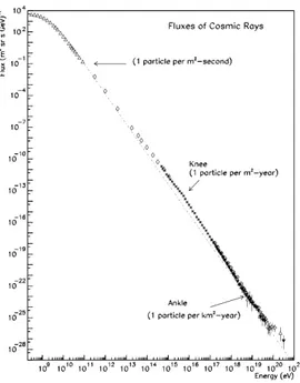
The prominent feature of cosmic rays is the wide range of energy spectrum, spanning
from ∼ 0.1 GeV to ∼ 1012GeV, and the fact that it can be described by a simple power
law:
dN
dE ∝E
−α
where α is the spectral index.
Figure 1.2. Differential energy spectrum of all cosmic rays at top of the
atmosphere; the dotted line shows E−3. [3]
Figure 1.2 shows the flux of cosmic rays: knee and ankle are zones in which the spec-tral index changes, suggesting different acceleration mechanisms for different ranges of energies; below 10 GeV the flux is strongly modulated by the intensity and polarization of the solar activity.
For nuclei, α = 2.7 up to 1016eV and α = 3.0 for 1016eV < E < 1018eV [3], while for
electrons (e−
+ e+) α = 3.0 in the range 7 GeV − 1 TeV [4].
Composition and flux of cosmic rays are well explained by the standard theory of supernovae remnants and cosmic propagation within our galaxy: if positrons were only secondaries, their flux should be the same of the primaries, plus a steepening due to the propagation and energy losses, so it is expected to be monotonically decreasing; any
dif-ferent behaviour of positrons spectrum, and thus of positrons fraction, i.e. e+
/(e−+e+), would suggest some source of primary positrons.
1.2. Dark matter
The study of the rotation velocity of galaxies have shown that this velocity remains constant with increasing distance from the center of the galaxy.
Assuming a spherical symmetry and all the mass of the galaxy concentrated in the nucleus (in effect, the mass of the disc is negligible compared to the mass of the nucleus), Newtonian mechanics predicts the rotation velocity to be
v(r) =
√
GM (r) r
where M (r) = ⎧ ⎪ ⎪ ⎪ ⎪ ⎨ ⎪ ⎪ ⎪ ⎪ ⎩ 4
3πρr3 inside the nucleus
Mtot outside the nucleus
So, v(r) ∼ r−1/2 in the galaxy disc, but observations contradict this hypothesis.
Figure 1.3. Rotation velocity of the galaxy NGC 7331, along with a
three-parameter dark halo fit (solid curve); dashed, dotted and dashed-dotted lines represent the velocity of various components (respectively:
visible, gas, dark halo).[5]
As can be seen in the figure 1.3, experimental data are compatible with a spherical halo of invisible (dark) matter, assuming a density distribution of an isothermal sphere
ρ(r) = ρ0[1 + (r rc ) 2 ] −1
where ρ0 is the central halo density and rc is halo core radius: this distribution is a
solution of the isothermal Lane-Emden equation.
There are mainly three hypothesis about the nature of dark matter (DM): (1) MOND (Modified Newtonian Dynamics)
This hypothesis requires no DM, but predicts alterations of the gravitational interactions at big distances.
The galaxy cluster 1E 0657-56 (figure 1.4), better known as Bullet Cluster, was originated from the collision between two smaller galaxy clusters and is claimed to be the best evidence against this theory: indeed, no MOND model seems to correctly account for the displacement of the center of the total mass from the center of the baryonic mass peak.
(2) MACHOs (Massive Astrophysical Compact Halo Object)
The missing mass could be made up of gas, JLO (Jupiter Like Objects), dwarf stars and black holes, since all these objects emit little or no electromagnetic radiation.
Microlensing measures excludes MACHOs with masses between 0.6 · 10−7 and
Figure 1.4. Bullet Cluster: in red the clouds of hot x-ray emitting gas,
in blue the distribution of dark matter inferred by observations of
gravi-tational lensing of background galaxies.[6] [7]
Big Bang Nucleosynthesis (BBN) constrains the fraction of the baryonic mat-ter (BM) in the Universe, using the cosmic abundance of light elements (D,
3He,4He,7Li), thus putting a limit on gas and JLO contribution to DM.
Com-bining BBN studies with CMB (Cosmic Microwave Background), BAO (Bary-onic Acoustic Oscillation), SNe Ia (Supernovae Type Ia) and Hubble Space Telescope observations (see figure 1.5), the WMAP experiment concludes that
Ωb=0.0456 ± 0.0016 (BM fraction) while ΩDM =0.227 ± 0.014 (DM fraction) [9]
(the remaining fraction is due to the so called dark energy).
These results exclude MACHOs as the answer to the DM problem.
Figure 1.5. 68.3%, 95.4% and 99.7% confidence level contours on ΩΛ
andΩM =ΩDM +Ωb obtained from CMB, BAO and SNe Ia.[10]
(3) Big Bang Relics
This term refers to all particles that exited from the equilibrium in the past and now freely stream in the Universe: neutrinos are the most known of them, but
their tiny mass make their contribution smaller than the baryonic matter one; other non-standard particles are Kaluza-Klein particles, axions, sterile neutri-nos and WIMPs [11].
WIMPs (Weakly Interacting Massive Particles) are the most promising candi-dates of DM: they are a generic type of particles that interact only via weak force, gravity and possibly other unknown forces no stronger than the weak force.
WIMPs are thought to be supersymmetric particles [12], thus conserving
R-parity1: supersymmetry (SUSY) is a theory beyond the Standard Model (SM)
predicting every SM particle to have a massive partner with its spin lowered by 1/2. Because WIMPs can not interact electromagnetically or strongly, they must be neutral and colorless; furthermore, they must be stable or have a mean lifetime greater than the age of the Universe, otherwise their decay product would have been already detected: the LSP (Lightest Supersymmetric Parti-cle), like the neutralino, has these properties, so it is the main WIMP candidate. 1.2.1. DM searches. DM search is an active field of research, with many experi-ments being carried on, both on Earth and in orbit.
Searches for WIMPs can be divided in three groups: (1) Direct searches
Direct searches aim to detect elastic scattering of WIMPs with nucleons. In order to remain in the Galaxy, WIMPs must have a velocity smaller than the
escape velocity, so they have v ≲ 300 km/s. Assuming MW IM P ≫ mp, WIMPs
transfer an energy E ≈ 2A keV to a nucleus at rest with a mass A; usually experiments look for a daily or even annual modulation in the signal due to the motion of the Earth in the Galaxy DM halo.
Detectors for these experiments are required to be sensitive to keV energies, to be radio pure in order to reduce the background and to have a big mass since the expected rate is roughly 1 event per day per kg of detector.
DAMA/LIBRA experiment is up to date the only one to claim the detection of a clear modulation.
Figure 1.6. Experimental model-independent residual rate of the
single-hit scintillation events; the black line is the best fitted oscillation.[13]
Recently, CoGeNT [14] and CDMS [15] saw small excesses, compatible with DAMA/LIBRA signal and with null signal from XENON10, pointing to
a DM candidate with mass MW IM P ∼ 5 ÷ 10 GeV [16]; the CRESST result,
which cannot be explained only by background, suggests different values in the WIMP mass-cross section parameter space.
(2) Indirect searches
These searches make use of the annihilation of DM particles in photons (HESS,
Figure 1.7. WIMP parameter space for various direct DM searches
ex-periments.[17]
MAGIC, Fermi), charged pairs (HEAT, PAMELA, AMS-02, Fermi) and neu-trinos (ANTARES, IceCube).
Modeling the flux of particles produced by the annihilation is very difficult, since the knowledge of DM annihilation cross section, DM density in the Galaxy and transport properties are required; in fact, the number N of events as a function
of the observed energy Eobs can be written as:
dN dEobs = ⟨σv⟩(Eprod) M2 ∫ ρ 2T i(Eprod, Eobs)dV
where ⟨σv⟩ is the thermally averaged annihilation cross section, v, M and ρ are
respectively the velocity, mass and density of DM and Ti is a transport term
describing how the particle energy changes from the production (Eprod) to the
detection (Eobs).
Various simulations have shown that DM tends to form clusters, so the cross
section is enhanced by the Sommerfeld effect2: this can be parametrized by
multiplying σ with a boost factor B; furthermore a high DM density increase the annihilation rate simply because there are more particles in the same volume. A recent study suggests that another source for the boost factor can be the conversion of heavier DM particles in lighter ones at a late time after the thermal decoupling, thus increasing the relic density [18].
As of now, the only sign of a possible DM annihilation has come from HEAT, PAMELA and Fermi positrons fraction: see section 1.3.
(3) Collider searches
These type of experiments rely on producing supersymmetric particles from the collision of highly energetic beams; the long decay chain of SUSY parti-cles is exploited, looking for events with many jets and MET (missing energy transverse). In particular, the LSP does not leave any trace in the detector, as behaving like a neutrino, and the only signature for its discovery is provided by the distribution of missing energy.
Comparisons of latest LHC data (1 fb−1) with direct searches results, constrain
the allowed values of LSP mass and cross section, although these limits strongly depend on the SUSY model analyzed.
For example, according to MSSM (Minimal Supersymmetric Standard Model),
2The Sommerfeld enhancement is a non relativistic quantum behaviour that accounts for the effect
of a potential on the interaction cross section: indeed, an attractive potential increases the probability for two particles to interact
DAMA/LIBRA and COGENT favor a neutralino with a Higgs mediated
anni-hilation and a high tan β3, but LHC data disfavors a high tan β [19]; in pMSSM
(phenomenological MSSM), LHC data, constrained by CDMS and XENON 100, favor a heavy neutralino with low neutralino-proton cross section [20].
1.3. Experimental results of positrons fraction
As reported in paragraph 1.2.1, positrons fraction can be used to detect DM annihi-lation.
In 2009, the PAMELA experiment (Payload for Antimatter Matter Exploration and Light-nuclei Astrophysics) published the first measurement of the positrons fraction up to 100 GeV: instead of decreasing, their fraction results to increase with energy from 10 GeV up.
Figure 1.8. Positrons fraction: red points are PAMELA data, black line
is the theoretical prediction for a pure secondary production of positrons
without reacceleration. [21]
Despite the error in the last bin is ∼35%, PAMELA result clearly disagree with the the-oretical expectations; since the collaboration excluded a proton contamination in their positrons set, this means that the positron component in cosmic rays is not correctly described by the standard theory.
At the end of the summer of 2011, Fermi LAT (Large Area Telescope) confirmed the PAMELA result up to 200 GeV (see figure 1.9).
Actually, these results are not yet a conclusive proof of DM annihilation: there are some criticalities in explaining this rise due to DM: the main concern is coming from the non observation of the same behaviour for the p/(p + p) ratio.
Furthermore, the increase with energy of the e+
/(e−+e+)ratio could also be explained
by astrophysical effect, involving one or more pulsars.
Pulsars are neutron stars with a high rotational velocity, thus creating a strong magnetic field surrounding the star. Electrons accelerated in the magnetosphere emit synchrotron
radiation, which in turn convert in e+e− pairs; around the magnetic axis there is a
narrow region in which field lines are open, so these pairs can escape from the star magnetosphere: positrons spectrum from pulsars can be described by a power law with
Figure 1.9. Positrons fraction: red points are Fermi data, shaded band
is the total uncertainty while bars are statistical errors.[22]
a cut-off at high energies.
The AMS-02 experiment
The Alpha Magnetic Spectrometer (AMS-02) is a cosmic rays detector built to operate in space; in May 2011 it was installed on the International Space Station (ISS) during the STS-134 NASA Endeavour Shuttle mission and, few days after, it started taking data. AMS-02 is the successor of AMS-01, a simpler detector that flew in June 1998 on the Shuttle Discovery (NASA mission STS-91).
The experiment will run at least 10 years, in order to obtain very precise measurements of cosmic rays spectra up to TeV scale.
The main research fields of AMS-02 are three: (1) Dark matter
Looking at spectra of the most rare cosmic rays components (like p, e+
, γ,d),
AMS-02 will be able to detect any deviation from the smooth energy spectra, a possible mark of DM annihilation (see sections 1.2.1 and 1.3).
Looking at cosmic rays anisotropies, it might be possible to discriminate be-tween astrophysical sources and DM sources.
(2) Antimatter
The Big Bang theory, strongly supported by experimental data (like Cosmic Microwave Background Radiation), predicts that at the beginning of the Uni-verse there was an equal amount of matter and antimatter, but until no trace of antimatter domains has been found in the Space.
The Standard Model of particle physics predicts a small CP violation which implies a different behaviour of matter and antimatter, but this violation is not enough to explain the asymmetry we see at the present.
Detecting anti-nuclei with Z > 1 would be a proof of the existence of antimatter domains in the early period of the Universe, since the probability of production of these anti-nuclei by interaction of cosmic rays with the interstellar medium is negligible.
(3) Cosmic rays
A precise knowledge of nuclei and isotopes spectra, in particular B/C and
10Be/9Be ratios, will allow a better understanding of cosmic rays propagation
within the galaxy.
2.1. Detector description The AMS detector is based on two fundamental requirements:
● Minimal material along the particle trajectory so to minimize background
in-teractions and to avoid large angle multiple scattering.
● Multiple measurements of momentum and velocity for an efficient background rejection and a better reliability in the measurement of these fundamental quan-tities.
To fulfill these requirements, AMS is equipped with many sub-detectors: a transition radiation detector (TRD), a time of flight (TOF), a silicon tracker (TRK) placed in a permanent magnet, an anti-coincidence counter system (ACC), a ring imaging Cherenkov counter (RICH) and an electromagnetic calorimeter (ECAL).
These detectors are assembled in the AMS-02 apparatus as shown in figure 2.1.
TRD: Transition Radiation Detector TOF: (s1,s2) Time of Flight Detector TR: Silicon Tracker ACC: Anticoincidence Counter MG: Magnet AST: Amiga Star Tracker RICH: Ring Image Cherenkov Counter EMC; Electromagnetic Calorimeter TOF: (s3,s4) Time of Flight Detector (Exploded View) TRD M-Structure Scintilators Photomultipliers
ACC Photomultipliers Star
Tracker Tracker AC C M ag ne t H e Ve ss el Radiator Reflector
Lead / Fiber Pancake
Photomultipliers
Photomultipliers
R.Becker 09/05/03
A star tracker (AST) provides an angular resolution for the FOV (field of view) of few arc seconds, acquiring the images of the stars and comparing them with an on-board astrometric star catalog.
AMS-02 is built to withstand the strong vibrations at the launch and the wide range of temperatures expected during its operations in Space: a system of heaters and radiators allows to maintain all detectors and their electronics in their operational temperature ranges.
To ensure electronics reliability in the high ionizing environment of Space, redundancy of each electronic sub-system is implemented.
2.1.1. Transition Radiation Detector. Transition radiation (TR) is the elec-tromagnetic radiation that is emitted when charged particles transverse the boundary between two media with different dielectric properties. The probability for a particle to emit a TR photon at a single interface is very small (1 %), so usually a multilayer structure is used, as showed in figure 2.2.
Figure 2.2. Principle of operation of TRD.
TRD is composed of 328 modules (see figure 2.3) with lengths ranging from 0.8 and 2
m, each containing 16 straw tubes filled with 80 % Xe and 20 % CO2 and operating at
1600 V. Modules are arranged in 20 layers: the lower and upper four ones are oriented parallel to the AMS-02 magnetic field, while the middle 12 ones are perpendicular to the field so to provide 3D tracking.
With this multilayer structure, the TR emission probability is enhanced up to 50 %.
Figure 2.3. TRD module with 16 straw tubes.
Using a likelihood analysis, TRD is able to discriminate up to 250 GeV between elec-trons/positrons and hadrons with a rejection power greater than 100, as can be seen in figure 2.4. [23]
Figure 2.4. TRD proton rejection.
2.1.2. Time of Flight. The TOF system is composed of four roughly circular planes of scintillating material (see figure 2.5): two planes are positioned above the permanent magnet (upper TOF) and two below the permanent magnet (lower TOF).
Each plane has a sensitive area of 1.2 m2 and in each plane paddles are overlapped by
0.5 cm to avoid geometrical inefficiencies. For efficient background rejection and for a rough estimation of the tracks incoming point, the paddles in the two adjacent planes are perpendicular.
Each paddle is read at both ends by two PMTs, able to operate in the residual field of the permanent magnet (up to 3 kG).
(a) Upper TOF (b) Design of a paddle
Figure 2.5. TOF detector.
TOF provides the fast trigger for charged particles and, thanks to its excellent time resolution (120 ps), is able to distinguishes downgoing particles from upgoing ones at a
level of 10−9. Furthermore, TOF provides a β measurement with a few % of resolution.
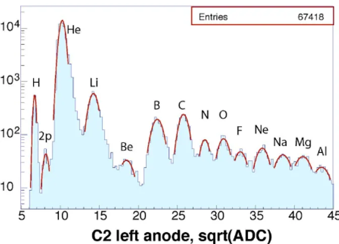
The measurement of the amount of collected light allows nuclei absolute charge deter-mination up to Z ≈ 15 [24], as the energy deposited in the paddles is proportional to the collected light and follows the Bethe-Bloch formula
−dE ρdx =K Z2 β2 Zmed A { 1 2ln ( 2mec2β2γ2Tmax ⟨I⟩2 ) −β2−δ 2}
where ρ, Zmed, A and ⟨I⟩ are respectively the density, atomic and mass number and
mean ionization energy of the material traversed, δ is a density correction and Tmax is
maximum kinetic energy transferred to an electron in a single collision. Figure 2.6 shows the good separation between different charge measurements.
Figure 2.6. Square root of the integrated charge measured at test beam.
2.1.3. Silicon Tracker and permanent magnet. The tracker is immersed in a uniform magnetic field generated by a permanent magnet made of 6400 high-grade Nd-Fe-B block (see figure 2.7a); the field is 1.5 kG along X axis (so Y is the bending direction) and fulfill the NASA requirements: a negligible dipole moment (in order to not create a torque on the ISS) and a leakage field at a distance of 2 m from the center of the magnet smaller than 3 G (to avoid interferences with the life support system of the astronauts).
The bending power of the magnet is 0.15 Tm2.
The AMS silicon tracker is the largest one built for a Space experiment: the major challenges were to maintain the required mechanical precision (despite the strong vibra-tions during the launch) and low-noise performance in this large scale application.
Tracker is composed of 41 x 72 x 0.3 mm3 double-sided silicon micro-strip sensors, for a
total detection area of ∼ 6.4 m2. For readout and biasing, the silicon sensors are grouped
together in ladders designed to match the cylindrical geometry of the magnet, for a total of 192 read-out units. The ladders are installed in 9 layers. 7 layers are placed inside the magnetic field (inner tracker). One external layer is placed on top of TRD, and the other one is placed on top of ECAL.
(a) Magnetic field orienta-tion and intensity.
(b) Plane 2 with ladders and readout channels.
Figure 2.7
An important feature of the tracker is the Laser Alignment System (TAS): the carbon fiber support structure of the tracker can have excursions up to 30 µm, mostly due to
change in thermal conditions, so it is necessary to realign the ladders and the planes; the laser realignment is performed coincident with data taking.
Each particle trajectory point is determined with an accuracy better than 10 µm in the bending direction (Y), and 30 µm in the non bending one (X).
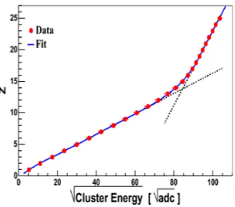
The tracker, like the TOF, provides also absolute charge information up to Z = 25 (see figure 2.8).
Figure 2.8. Relation of the corrected cluster energy and charge of ladder 1. A particle with charge q = ze and rigidity R = pc/q which moves in a uniform magnetic field B follows an helix trajectory with radius of curvature
ρ = R
Bcsin θ
where θ is the angle between the particle momentum and B; AMS magnetic field is not homogeneous, so the trajectory is more complicated, but if B is known, the reconstruction of the full trajectory can be used to obtain R.
If σpos is the spatial resolution of the tracker in the bending direction, l the lever arm
inside the magnet (from plane 2 to plane 8) and L the full lever arm (from plane 1 to plane 9), the relative uncertainty on R can be written as
∆R
R ∝
Rσpos
BlL
When ∆R/R = 1, the corresponding value of R is called Maximum Detectable Rigidity (MDR).
For the inner tracker MDR ∼ 200 GeV, while for full tracker MDR ∼ 2 TeV; figure 2.9
shows the relation between generated MC rigidity (RM C) and measured rigidity: the
value of RM C at which the distribution becomes parallel to X-axis and begins to widen
is the MDR.
In the original project, AMS-02 should have had a superconducting magnet (SCM), instead of a permanent one (PM), but this way the experiment would have been lasted only three years, due to the lifetime of the cryostat required to maintain fully functional the SCM. When it was decided that the ISS would have been continued its operations beyond 2020, the SCM was substituted with a PM, moving two layers outside the magnet in order to increase the lever arm and thus the MDR.
Figure 2.10 shows the comparison of the rigidity resolution between the SCM and PM configurations: the PM resolution (blue line), can be parametrized as
∆R
) MC log10(R 1 1.5 2 2.5 3 3.5 ) meas inn log10(R 1 1.5 2 2.5 3 3.5 4 4.5 5 1 10 2 10 3 10
(a) Inner tracker.
) MC log10(R 1 1.5 2 2.5 3 3.5 ) meas full log10(R 1 1.5 2 2.5 3 3.5 4 4.5 5 1 10 2 10 (b) Full tracker.
Figure 2.9. Relation between generated MC rigidity and measured rigidity. so that for R = 100 GV, the resolution is ≈ 15.7%.
Figure 2.10. Rigidity resolution comparison in blue the PM resolution,
in red the SCM one. The green area is the difference between the
resolu-tions of the two configuraresolu-tions. [25]
2.1.4. Anti-Coincidence Counter. The ACC is formed by 16 scintillation pad-dles arranged on a cylinder surrounding the tracker; ACC PMTs were selected to operate in magnetic field.
ACC has a very high efficiency in vetoing particles passing through AMS but not cross-ing all detectors; this veto is included in the AMS trigger, in order to reject particles outside the tracker acceptance.
2.1.5. Ring Imaging Cherenkov Counter. When a charged particle passes through a material at a velocity greater than the speed of light in that material, Cherenkov ra-diation is emitted in a cone of aperture angle:
cos(θC) = 1
βn(ω)
where n is the refractive index of the material.
The number of photon Nγ emitted in a range of frequency dω and for a traversed length
dxis:
d2Nγ
dωdx =αemZ
2sin2
(θC) where Z is the charge of the particle.
Therefore, RICH can measure both the velocity (with a resolution σβ/β ∼0.1%/Z) and
the absolute charge of the particle (up to Z = 26 with a charge confusion less than 10%), independently from TOF and tracker; figure 2.11 shows the good agreement in charge measurement between RICH, TOF and tracker.
(a) TOF - RICH (b) Tracker - RICH.
Figure 2.11. Correlations between charge measurements of RICH and
TOF/tracker
RICH has a truncated conical shape where the top plane contains a silica Aerogel
(SiO2 ∶2H2O) and NaF blocks, while the lower one hosts light guides and PMTs. The
lateral surface is covered by a mirror, in order to maximize the acceptance of the emitted photons. Given this structure, upgoing particle cannot be detected; as a consequence, RICH improves the discrimination power of the TOF in the identification of upgoing and downgoing particles.
In the center of the lower plane, there is a hole to let particles go unaffected to ECAL.
Figure 2.12. RICH structure and reconstruction techniques.
2.1.6. Electromagnetic Calorimeter. ECAL is a lead-scintillating fiber sam-pling calorimeter with high granularity, that allows a precise 3D imaging of the lon-gitudinal and lateral profile of the showers, providing a good energy resolution and a high hadrons rejection power.
2.1.7. Trigger system. The AMS-02 trigger recognizes charged particles by a log-ical combination of TOF, ACC and ECAL responses, producing Fast Trigger (FT) and
Level 1 Trigger (LVL1): the trigger system is very flexible, thanks to the possibility of
using masks.
Electromagnetic showers in ECAL
3.1. Calorimeter structure
The calorimeter ECAL is made of lead, fiber and glue in a volume ratio of 1:0.57:0.15
cm3; it has an average density of ∼6.8 g/cm3 and a radiation length X
0 of about 1 cm.
The active volume is built up by 9 superlayers (SL), each consisting of 11 grooved lead foils (1mm thick) interleaved by 1mm plastic scintillating fibers. Fibers are glued by means of optical cement and are stacked alternatively parallel to the Y-axis (5 SL) and X-axis (4 SL). Each superlayer is designed as a square parallelepiped with 68.5 cm side
and 1.85 cm height, for a total active dimension of 68.5 x 68.5 x 16.7 cm3, corresponding
to ∼17X0for perpendicular incident particles. The ratio between the nuclear interaction
length and the radiation length is ∼26: this ensures that ∼50% of the hadrons does not interact in the calorimeter.
(a) Three superlayers.
(b) Cross section of the lead-fiber-glue composite structure.
(c) Exploded view of the mechanical support structure.
Figure 3.0. ECAL structure.
Each superlayer is read out by 36 Hamamatsu R-7600-00-M4 multianode PMTs (which have been chosen to fit ECAL granularity and to work in magnet fringing field), arranged alternatively on the two opposite ends to avoid mechanical interference. The coupling to fibers is realized by means of plexiglass light guides, that maximizes light collection and reduce cross-talks. Optical contact is enhanced by silicone joints positioned in front of light guides. Finally, PMTs are shielded from magnetic field by a 1 mm thick soft iron square parallelepiped tube, which also acts as mechanical support for the light collection
system.
Each anode covers an active area of 8.9 x 8.9 mm2, corresponding to ∼35 fibers, defined
as a cell (the minimum detection unit).
In total the ECAL is subdivided into 1296 cells (324 PMTs) arranged in a 18x72 grid and this allows for an accurate 3D imaging-sampling of the longitudinal shower profile; a software program uses the energy deposit in every cell to define the cells belonging to a shower: this is called clustering phase.
Figure 3.1. Exploded view of the light collection system.
PMT High Voltage is provided by a custom programmable HV power supply, which
sets the average HV PMT value to around 700V, corresponding to a gain factor ∼2 · 105.
Only 240 HV channels out of 324 are independent.
The front-end electronics and digitalization cards are directly located behind the PMT base. In order to obtain the necessary energy resolution on Minimum Ionizing Particles (used for detector performance monitoring and equalization) and to measure energies up to 1 TeV using standard 12 bit ADC, digitization is performed at two different gains: High Gain for low energy measurements (up to ∼2 GeV per cell) and Low Gain, when HG saturates, for highest ones (up to ∼66 GeV per cell), with a conversion factor
HG/LG ∼33.
Each PMT last dynode signal is also readout and its information is used to have a re-dundant signal in case of anode breakdowns.
Front-end electronics sends ADC signal to the ECAL Data Reduction board (EDR), where ”pedestal calculation” and ”zero suppression” are performed. Last, dynode sig-nals are sent to the ECAL Intermediate Board (EIB) where they are compared with a programmable threshold to obtain trigger bits. Using these bits, the ECAL TRiGger board (ETRG) generates then the Fast and Level1 trigger bits, which are sent to the JLV1 AMS-02 trigger board where the LVL1 trigger is formed.
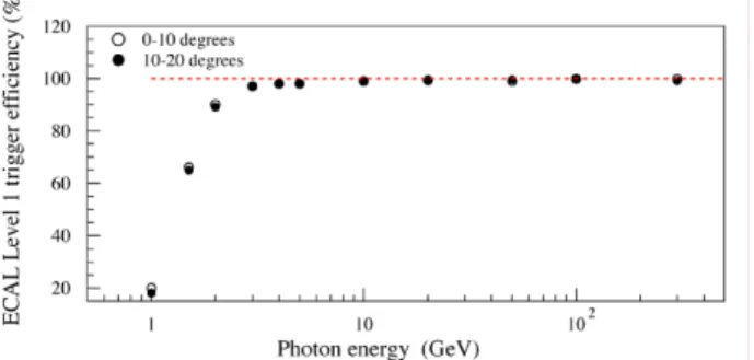
Furthermore, the calorimeter provides a stand-alone photon trigger. The trigger effi-ciency is 90% at 2 GeV and more than 99% for energies greater than 10 GeV.
Figure 3.2. ECAL trigger efficiency for photons of different energies
3.2. ECAL performances
In figure 3.3, a typical longitudinal electromagnetic shower profile for an electron at 6 GeV in ECAL is shown.
Figure 3.3. Typical longitudinal electromagnetic shower profile for an
electron of 6 GeV in ECAL.
The relation between the maximum of the shower and the energy of the shower (see appendix A) can be used to evaluate ECAL radiation length, by fitting the measured maximum position as a function of the energy of the particle:
Figure 3.4. Determination of the radiation length in layer units from
the 2007 test beam.
As is shown in figure 3.4, for ECAL X0 results to be X0=1.07 ± 0.01 l.u ∼ 1 cm. [26]
According to the Rossi function, the shower energy not contained in ECAL due to the
rear leakage is negligible at low energies, but it becomes important at high energies: as
a consequence a correction to the detected energy is required.
To recover the missing energy, the measured energy is parameterized as a quadratic
function of the last 2 layers energy fraction (EL2L/Erec):
Eincoming Erec =α + βEL2L Erec +γ (EL2L Erec ) 2
The parameters α, β and γ were evaluated in a dedicated test beam (2007), where
Eincoming was corresponding to the nominal beam energy.
The figure 3.5 shows the dependence on EL2L/Erec of the correction factor and the
corrected energy distribution.
Figure 3.5. Energy leakage correction factor as function of the fraction
of energy released in the last two layers (left). The correction recovers the energy tail due to the longitudinal leakage (right).
Analogous to the rear leakage is the lateral leakage, i.e. when the shower partially is escaping from the lateral sides of ECAL.
Lateral leakage is recovered during the clustering phase with a mirror technique: in a single layer, the cluster is symmetrized with respect to the maximum cell.
Finally, the energy resolution of ECAL results to be [26]:
σ(E) E = 9.9% √ E(GeV) ⊕1.5%
The segmentation of ECAL allows to compute the angle of the shower i.e. the incli-nation of the axis of the shower. The axis is reconstructed in the following way: first, for each layer the center of the energy deposit is found, computing the first moment of the energy distribution in the most energetic cluster (so that fluctuations are not taken into account); then, all centers are fitted with a straight line.
The calorimeter angular resolution, ∆θ68, is defined as the angular width around the
incidence beam/particle angle containing 68% of the reconstructed angles; at 0○ degrees
is [26]: ∆θ68(E) = 14.5 ○ E(GeV) ⊕ 6.3○ √ E(GeV) ⊕0.42○
while for beams not perpendicular to the calorimeter gets better, because oblique showers release more energy in the calorimeter.
Leptons-hadrons discrimination
The biggest difficulty in the measurement of the positrons fraction consists with
pro-ton contamination of the e+ sample due to the high protons-to-positrons ratio, of the
order of 103
÷104. Therefore AMS-02 needs to select a very low signal within a very
high background. In order to achieve this discrimination, a proton rejection factor of
105÷106 is required so to keep the error in the positrons counting due to the background
at the percent level.
TRD, TRK and ECAL are the fundamental sub-detectors used for this purpose: TRK
provides the sign of charge, TRD and ECAL allow to separate e+
/e−from p/p.
This chapter will be focused on the ECAL rejection power.
4.1. Differences between electromagnetic and hadronic showers
As stated in section 3.1, half of the protons when entering the calorimeter will behave as MIPs and therefore will not initiate a shower. These protons are easily recognized by ECAL, thanks to their low energy deposit. In fact, the loss of energy of a MIP in a layer of matter is described by the Landau distribution: in particular, the Landau peak corresponds to the most probable value (MPV) of energy deposit. In ECAL, the MPV for a perpendicular MIP in a cell is ≈ 7 MeV.
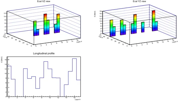
A MIP is shown in figure 4.1: the two upper plots show the XZ and YZ views of the calorimeter, giving a 3D display of the energy deposit, while the lower plot is the longitudinal profile. Layer # 0 2 4 6 8 10 12 14 16 Cell # 0 10 20 30 40 50 60 70 E [MeV] 0 2 4 6 8 10 12 Ecal XZ view Layer # 0 2 4 6 8 10 12 14 16 Cell # 0 10 20 30 40 50 60 70 E [MeV] 0 2 4 6 8 10 12 14 16 18 Ecal YZ view Layer # 0 2 4 6 8 10 12 14 16 E [MeV] 0 2 4 6 8 10 12 14 16 Longitudinal profile
Figure 4.1. A 25 GeV proton MIP in ECAL.
Proton identification becomes difficult when the proton interacts, producing a high
en-ergy π0, which subsequently decays in 2γ. Apart from this specific interaction, hadronic
cascades have a different longitudinal and lateral shape with respect to those induced by electrons/positrons: these topological differences can be exploited by the fragmented structure of ECAL so to separate leptons from hadrons.
Figures (4.2) and (4.3) show the typical electron shower shape and the typical proton cascade: Layer # 0 2 4 6 8 10 12 14 16 Cell # 0 10 20 30 40 50 60 70 E [MeV] 0 200 400 600 800 1000 1200 1400 1600 1800 2000 2200 Ecal XZ view Layer # 0 2 4 6 8 10 12 14 16 Cell # 0 10 20 30 40 50 60 70 E [MeV] 0 200 400 600 800 1000 1200 1400 1600 1800 2000 2200 Ecal YZ view Layer # 0 2 4 6 8 10 12 14 16 E [MeV] 0 500 1000 1500 2000 2500 3000 3500 Longitudinal profile
Figure 4.2. A 25 GeV electron interacting in ECAL.
Layer # 0 2 4 6 8 10 12 14 16 Cell # 0 10 20 30 40 50 60 70 E [MeV] 0 100 200 300 400 500 600 700 800 900 Ecal XZ view Layer # 0 2 4 6 8 10 12 14 16 Cell # 0 10 20 30 40 50 60 70 E [MeV] 0 100 200 300 400 500 600 700 800 Ecal YZ view Layer # 0 2 4 6 8 10 12 14 16 E [MeV] 0 200 400 600 800 1000 1200 1400 1600 Longitudinal profile
The electron shower results to be almost fully contained in the calorimeter, while this is not the case for the protons. Actually, interacting protons release in average half of their energy when showering in ECAL; it should also be noted that the proton shower is wider than the electron one.
4.2. Events preselection
The lepton-hadron discrimination procedure may be seen as a three-step process: a) choice of some variables derived from the information provided by the calorimeter (i.e.
deposit energy in each cell), b) study, for each variable, of the different answer for e+
/e− and for p, c) selection of cuts on each variable to maximize both the efficiency of the
signal (e+
/e−) and the rejection of the background (p).
In order to do this, a clean sample of events (signal and background) must be selected. Since positrons are very few and are contaminated by a huge background, the procedure has been studied looking at electrons, which produce the same kind of signal as the one from positrons.
The final goal is to have a measure of the selected variables as a function of the energy. From the first six months of data taking, a sufficient statistics is available only up to 100 GeV.
The selection of clean events collected on the ISS was divided in three steps, which aims to not introduce bias:
(1) TRK selection
● There must be only one reconstructed track in the tracker (to avoid
over-lapping particles or bad tracker reconstructions) with a good pattern in the inner tracker (i.e. at least 4 hits on the X direction and at least 5 on the Y
direction) and a normalized χ2 less than 5.
● The rigidity (R) derived from the track sagitta must be ∣R∣ > 3 GV, so to
remove low momentum particles, strongly affected by multiple scattering.
● The track must cross the geometrical acceptance of the first layer of ECAL.
(2) ECAL selection
● At least one shower must be reconstructed in ECAL: if more than one
shower is present, the one with the highest energy is selected.
The number of events with more than one shower is very small (≲ 3%). For these events, the ratio between the energies of the two showers is peaked at
∼3%: therefore, with the rejection of the second shower, the error on the
energy measurement is comparable to the energy resolution of the calorime-ter.
● Entry and exit points of the selected shower must be 2 cells (one PMT) far
from the border (i.e. a fiducial volume is defined).
● A quality cut on the track-shower matching is requested: the track is
ex-trapolated at the center of gravity of the shower (defined as the first moment of the energy deposit distribution in the three directions) and required to have a distance from the shower axis not greater than 2 PMTs.
This is a loose cut, but allows to reject showers not belonging to the track or badly reconstructed from ECAL.
(3) TRD selection
● Only one reconstructed track in TRD is required, to avoid confusion in the
requests on its qualities (cut on the number of hits and on the normalized
χ2 of the TRD track).
● TRD track and tracker track are extrapolated at the upper TOF layer and
their distance must be less than 4 cm.
Finally, the selected events are divided in a (theoretically) clean electron sample and a proton sample using the TRD, which provides three types of likelihood: e/p likelihood (to separate electrons from protons), e/He likelihood (to separate electrons from Helium) and p/He (to separate protons from Helium).
First, Helium is rejected cutting on e/He and p/He likelihoods, leaving an Helium
con-tamination at the level of 10−5; next, the reconstructed energy must be above 5 GeV, so
to discard all MIPs.
A common cut on the ratio between reconstructed energy and measured rigidity (∣E/R∣ > 0.5) is applied: this loose cut selects among all protons those which are more easily mis-taken for electrons in ECAL.
Subsequently, electrons are tagged requiring a negative rigidity and a 90% efficiency cut on TRD e/p likelihood (see figure 4.4), while for protons a positive rigidity and the complementary cut on TRD e/p likelihood are requested.
TRD Likelihood 0 0.2 0.4 0.6 0.8 1 1.2 1.4 1.6 1.8 2 2.2 2.4 # events 1 10 2 10 3 10 4 10 5 10 Electrons Protons
Figure 4.4. TRD e/p likelihood for negative rigidity particles (blue line)
and positive rigidity particles (red line): the black dashed line shows the
90% efficiency cut; the small bump at 1 in the negative rigidity particles is
compatible with an anti-proton contamination which is anyway discarded by the TRD likelihood cut.
4.3. First approach: simple cuts
ECAL provides 1296 raw variables (the energy deposit in each cell), which can be combined in many ways to obtain information about the longitudinal and lateral shower development.
First, a small set of variables has been chosen:
● ShowerMean: Longitudinal mean of the shower in layer units, i.e. the mean
of the layers l weighted by the energy deposit of the shower El in the layers:
ShowerMean = µ = ∑llEl
● ShowerSigma: Longitudinal dispersion of the shower in layer units, i.e. the standard deviation of the layers l weighted by the energy deposit of the shower
El in the layers: ShowerSigma = σ = ¿ Á Á À ∑l(l − µ)2El ∑lEl
● L2LFrac: Fraction of deposited energy in the last two layers.
● R3cmFrac: Fraction of deposited energy in a circle of 3 cm radius around the shower axis; this is roughly proportional to the Molière radius.
● NEcalHits: Number of hits in the calorimeter belonging to the shower. ● ShowerFootprint: A measure of the area covered by the shower, computed
as the determinant of the ”inertia tensor” of the deposited energy relative to the shower center of gravity (CoG):
Ij= ( σjj σjz σjz σzz ) where j = x, y and σij = cells ∑ k=1 (cki −bi)(ckj −bj)Ek cells ∑ k=1 Ek
ck= [ckx, cky, ckz]are the coordinates of the k-th cell of ECAL, while b = [bx, by, bz]
are the coordinates of the shower CoG; Ek is the deposited energy of the k-th
cell.
With these definitions, the footprint is
ShowerFootprint =√∣Ix∣ +
√ ∣Iy∣ and so it has the units of squared cells.
These variables depend on the energy of the shower, although some of them very weakly, thus the cut on each variable has been chosen so to retain in every bin of energy
∼99% of the signal.
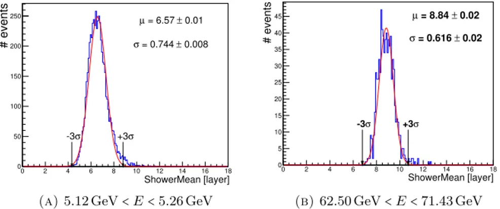
For this purpose, each variable distribution was fitted with a gaussian in every energy bin (slice), obtaining two cut values at ±3 σ as a function of energy (see figure 4.5).
ShowerMean [layer] 0 2 4 6 8 1012141618 # events 0 50 100 150 200 250 µ= 6.57±0.01 0.009 ± = 0.764 σ ShowerMean - 5.00 < E [GeV] < 5.05 ShowerMean [layer] 0 2 4 6 8 10 12 14 16 18 # events 0 50 100 150 200 250 µ= 6.57±0.01 0.008 ± = 0.744 σ ShowerMean - 5.21 < E [GeV] < 5.26 σ +3 σ -3
(a) 5.12 GeV < E < 5.26 GeV
ShowerMean [layer] 0 2 4 6 8 10 12 14 16 18 # events 0 5 10 15 20 25 30 35 40 45 µ= 8.84±0.02 0.02 ± = 0.616 σ ShowerMean - 62.50 < E [GeV] < 71.43 σ -3 +3σ (b) 62.50 GeV < E < 71.43 GeV
Figure 4.5. Gaussian fit (red line) of two slices (blue line). µ and σ of
the fit are written in the right top corner, while two arrows indicate the
Finally, these cut values have been fitted, defining an upper and a lower cut dependent on energy. Figure 4.6 shows the upper and lower cut on ShowerMean as a function of 1/E (in this figure, electrons have negative energies): the black dashed lines are the ±3 σ bands within which events are selected.
] -1 1/E [GeV -0.2 -0.15 -0.1 -0.05 0 0.05 0.1 0.15 0.2 ShowerMean [layer] 0 2 4 6 8 10 12 14 16 18 1 10 2 10 3 10
Figure 4.6. ShowerMean distribution vs 1/E: the ∼ 99% signal
effi-ciency cut is shown with black dashed lines.
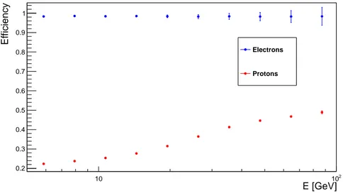
As it can be seen in figure 4.7, the efficiency on electrons is ∼ 99% and nearly flat, while that on the protons rises from ∼20% at 5 GeV to ∼50% at 100 GeV.
E [GeV] 10 102 E ff ic ie n c y 0.2 0.3 0.4 0.5 0.6 0.7 0.8 0.9 1 Electrons Protons
Figure 4.7. Efficiency of the ShowerMean cut on electrons (blue circles)
and protons (red circles); vertical bars are statistical errors.
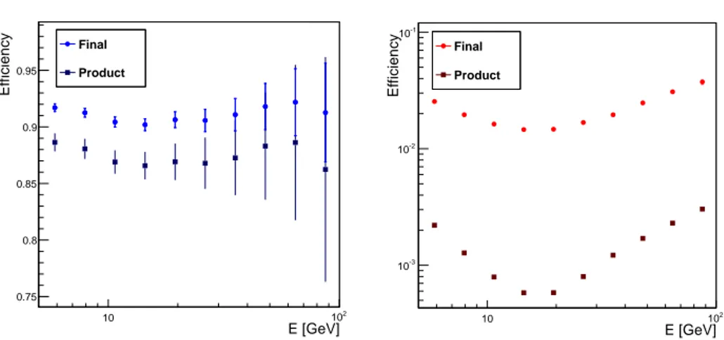
All cuts have been applied in sequence, in the order of the variables presentation done above; the final efficiency has been checked to not depend on the order of the sequence, as it was expected.
Figure 4.8 presents the efficiency of all cuts for electrons and protons; if these variables were independent from each other, the final efficiency would be simply the product of every single cut efficiency: as it can be seen, this is not the case, in particular for
E [GeV] 10 2 10 E ff ic ie n c y 0.75 0.8 0.85 0.9 0.95 Final Product E [GeV] 10 2 10 E ff ic ie n c y -3 10 -2 10 -1 10 Final Product
Figure 4.8. Final efficiency of all cuts for electrons (blue circles) and
protons (red circles) compared to the product of efficiencies of single cuts (dark blue and dark red squares).
protons, where the correlation between variables rises the final efficiency of one order of magnitude with respect to the efficiency in the hypothesis of uncorrelated variables.
Indeed, the variables for protons are correlated, as shown in figure 4.9; on the left, the distribution of ShowerSigma vs 1/E is displayed without any cut applied, while on the right, the same distribution after the cut on ShowerMean is presented: the effect of the ShowerMean cut on protons is clearly visible and not only changes the number of events, as it would be in the case of uncorrelated variables, but also modifies the distribution shape. ] -1 1/E [GeV -0.2 -0.15 -0.1 -0.05 0 0.05 0.1 0.15 0.2 ] 2 ShowerSigma [layer 1 2 3 4 5 6 7 8 1 10 2 10 3 10 ] -1 1/E [GeV -0.2 -0.15 -0.1 -0.05 0 0.05 0.1 0.15 0.2 ] 2 ShowerSigma [layer 1 2 3 4 5 6 7 8 1 10 2 10
Figure 4.9. Left: ShowerSigma distribution without any cut applied.
Right: ShowerSigma distribution after ShowerMean cut.
A simple cuts approach is not sufficient: to exploit the correlations between variables, a multivariate method for leptons-hadrons discrimination has been implemented.
4.4. Multivariate analysis: Boosted Decision Tree (BDT)
Multivariate analysis (MVA) techniques allow to study many statistical variables at the same time, taking into account the effect of all variables on the desired output, i.e.
their correlations: MVA methods are especially useful in the case of non-linear correla-tions.
In order to discriminate between two classes of events, one would like to find the best set of cuts to be applied, so to maximize the efficiency on one class (the signal S) and the rejection on the other (the background B): in a way, this is similar to a multidimensional fit.
A decision tree (DT) is a model born in data mining and machine learning fields: it is a very intuitive way to classify data, using a sequence of binary decisions to establish if a given set of variables describes better the signal instead of the background.
DTs accept as input a training sample of signal events and a training sample of back-ground events: both samples are grouped to create what is called the root node of a decision tree. At each step, the sample is divided in two sub-samples, cutting on the variable that gives the best separation gain (see below), thus producing two child nodes; the splitting continues until some conditions (for example, the minimum number of events allowed in a node or the maximum number of nodes created) are reached, then the last nodes, called leaf nodes, are tagged as S or B depending on the majority of events of one type or of the other.
Figure 4.10 shows an example of a decision tree: nodes 1 and 2 are child nodes with respect to the root node, while this one is a parent node for nodes 1 and 2.
Figure 4.10. Example of a decision tree.
A single step of a DT looks like the simple cuts approach, but one of the advantages of DTs is that instead of having a single set of cuts for the entire phase space of variables, one has multiple sets, so the correlations can be fully taken into account to achieve a better separation.
Another advantage of DT is its stability against poor discriminating variables, since these variables will be rarely used in node splitting.
There are different ways of measuring the separation gain of a cut: the most commonly used is the Gini index.
Defining the purity P as
P = ∑sws
where wsand wbare the weight of the signal and background events, then the Gini index is
G = P (1 − P )
At each step, all variables and all possible cuts are considered, then P is computed for the events passing the cuts and the best cut is chosen maximizing the separation gain:
Nparent nodeGparent node−Nleft child nodeGleft child node−Nright child nodeGright child node
This procedure could continue until a node has only signal or background events, so obtaining the best set of cuts that separate the root node exactly in the starting training samples; this set, however, is not generally the best one, since has been optimized on the events of the training samples and in principle could have a different behaviour on an independent sample (see figure 4.11): when this fact happens, the DT is said to be
overtrained.
Figure 4.11. Comparison of overtrained cut (left) and not overtrained
cut (right).
Overtraining means that the DT has learned to recognize as characteristics of the signal not only the real variables distributions, but also their statistical fluctuations: indeed, this is the main disadvantages of decision trees.
In order to overcome the stability problem of DTs, two other techniques have been introduced: boosting (which also increases the separation power) and bagging, hence the name of boosted decision tree (BDT).
Boosting constructs more than one tree (technically speaking, a forest of trees): when
a DT has been evaluated, the next tree re-weights the events according to the misclas-sification of the previous tree. There are many boosting algorithms, the most known of them is AdaBoost, which however degrades its performances in noisy settings: for this reason, in this thesis the GradientBoost algorithm has been chosen, thanks to its robustness against mislabeled events in the training sample.
Baggingis a resampling technique, where a BDT is trained more times on different
train-ing events randomly picked from the parent sample: this way, the statistical fluctuations are averaged and the resulting BDT is more stable.
The output of a BDT is a continuous distribution, like a likelihood: going from left to right, the probability of an event of belonging to background reduces, while that of belonging to signal increases.
BDT training has been performed with the TMVA [27] library provided by ROOT analysis tool [28].
4.4.1. BDT training and testing. As said before, calorimeter variables depend on the energy; in the simple cuts approach, the cut was energy dependent too, but there is no way to make the BDT aware of this fact. To resolve this problem, all signal variables have been normalized, removing the energy dependence.
As done in section 4.3, each variable X has been fitted with a gaussian in every energy
bin; the means µX(E) and sigmas σX(E) of the obtained gaussians have been fitted as
functions of energy (see figure 4.12).
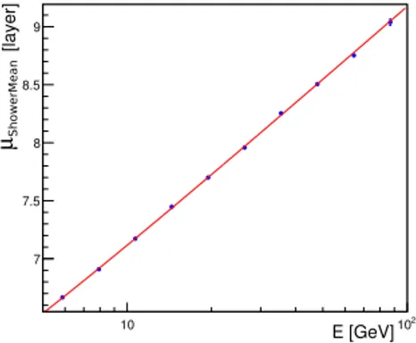
E [GeV] 10 102 [layer] µSho werMe a n 7 7.5 8 8.5 9
Figure 4.12. Fit of the mean µX(E) obtained from the gaussian fit of
the energy slices of the ShowerMean variable.
Finally, the following transformation has been applied
XNorm(E) = X(E) − µX
(E)
σX(E)
leading, for the signal, to a variable whose distribution is centered in zero and has a unitary sigma in every energy bin; the effect of this transformation is different on the background, since the protons variables behave distinctly from the electrons variables. The result of this normalization is shown in figure 4.13, while figure 4.14 shows the input variables for the BDT training for electrons (blue) and protons (red).
ShowerMean [layer] 4 5 6 7 8 9 10 11 12 13 Events / (0.09 layer) 0 0.01 0.02 0.03 0.04 0.05 0.06 5 < EnergyE < 9.1 9.1 < EnergyE < 20 20 < EnergyE < 42 42 < EnergyE < 65 65 < EnergyE < 100
(a) Before normalization.
ShowerMeanNorm [layer] -6 -4 -2 0 2 4 6 Events / (0.14 layer) 0 0.01 0.02 0.03 0.04 0.05 0.06 5 < EnergyE < 9.1 9.1 < EnergyE < 20 20 < EnergyE < 42 42 < EnergyE < 65 65 < EnergyE < 100 (b) After normalization.
Figure 4.13. Distribution of ShowerMean for signal in different energy
ShowerMeanNorm -6 -4 -2 0 2 4 6 8 10 12 0.485/ (1/N) dN 0 0.05 0.1 0.15 0.2 0.25 0.3 0.35 0.4 0.45 Signal Background ShowerSigmaNorm -15 -10 -5 0 5 10 15 0.776/ (1/N) dN 0 0.05 0.1 0.15 0.2 0.25 0.3 0.35 0.4 L2LFracNorm 0 10 20 30 40 50 60 70 80 90 2.42/ (1/N) dN 0 0.02 0.04 0.06 0.08 0.1 0.12 0.14 0.16 0.18 0.2 R3cmFracNorm -70 -60 -50 -40 -30 -20 -10 0 2.09/ (1/N) dN 0 0.05 0.1 0.15 0.2 0.25 NEcalHitsNorm -10 -5 0 5 10 15 0.744/ (1/N) dN 0 0.05 0.1 0.15 0.2 0.25 0.3 0.35 0.4 ShowerFootprintNorm -10 0 10 20 30 40 50 60 70 2.16/ (1/N) dN 0 0.02 0.04 0.06 0.08 0.1 0.12 0.14 0.16 0.18 0.2 0.22 0.24 (a) ShowerMean ShowerMeanNorm -6 -4 -2 0 2 4 6 8 10 12 0.485/ (1/N) dN 0 0.05 0.1 0.15 0.2 0.25 0.3 0.35 0.4 0.45 Signal Background ShowerSigmaNorm -15 -10 -5 0 5 10 15 0.776/ (1/N) dN 0 0.05 0.1 0.15 0.2 0.25 0.3 0.35 0.4 L2LFracNorm 0 10 20 30 40 50 60 70 80 90 2.42/ (1/N) dN 0 0.02 0.04 0.06 0.08 0.1 0.12 0.14 0.16 0.18 0.2 R3cmFracNorm -70 -60 -50 -40 -30 -20 -10 0 2.09/ (1/N) dN 0 0.05 0.1 0.15 0.2 0.25 NEcalHitsNorm -10 -5 0 5 10 15 0.744/ (1/N) dN 0 0.05 0.1 0.15 0.2 0.25 0.3 0.35 0.4 ShowerFootprintNorm -10 0 10 20 30 40 50 60 70 2.16/ (1/N) dN 0 0.02 0.04 0.06 0.08 0.1 0.12 0.14 0.16 0.18 0.2 0.22 0.24 (b) ShowerSigma ShowerMeanNorm -6 -4 -2 0 2 4 6 8 10 12 0.485/ (1/N) dN 0 0.05 0.1 0.15 0.2 0.25 0.3 0.35 0.4 0.45 Signal Background ShowerSigmaNorm -15 -10 -5 0 5 10 15 0.776/ (1/N) dN 0 0.05 0.1 0.15 0.2 0.25 0.3 0.35 0.4 L2LFracNorm 0 10 20 30 40 50 60 70 80 90 2.42/ (1/N) dN 0 0.02 0.04 0.06 0.08 0.1 0.12 0.14 0.16 0.18 0.2 R3cmFracNorm -70 -60 -50 -40 -30 -20 -10 0 2.09/ (1/N) dN 0 0.05 0.1 0.15 0.2 0.25 NEcalHitsNorm -10 -5 0 5 10 15 0.744/ (1/N) dN 0 0.05 0.1 0.15 0.2 0.25 0.3 0.35 0.4 ShowerFootprintNorm -10 0 10 20 30 40 50 60 70 2.16/ (1/N) dN 0 0.02 0.04 0.06 0.08 0.1 0.12 0.14 0.16 0.18 0.2 0.22 0.24 (c) L2LFrac ShowerMeanNorm -6 -4 -2 0 2 4 6 8 10 12 0.485/ (1/N) dN 0 0.05 0.1 0.15 0.2 0.25 0.3 0.35 0.4 0.45 Signal Background ShowerSigmaNorm -15 -10 -5 0 5 10 15 0.776/ (1/N) dN 0 0.05 0.1 0.15 0.2 0.25 0.3 0.35 0.4 L2LFracNorm 0 10 20 30 40 50 60 70 80 90 2.42/ (1/N) dN 0 0.02 0.04 0.06 0.08 0.1 0.12 0.14 0.16 0.18 0.2 R3cmFracNorm -70 -60 -50 -40 -30 -20 -10 0 2.09/ (1/N) dN 0 0.05 0.1 0.15 0.2 0.25 NEcalHitsNorm -10 -5 0 5 10 15 0.744/ (1/N) dN 0 0.05 0.1 0.15 0.2 0.25 0.3 0.35 0.4 ShowerFootprintNorm -10 0 10 20 30 40 50 60 70 2.16/ (1/N) dN 0 0.02 0.04 0.06 0.080.1 0.12 0.14 0.16 0.18 0.2 0.22 0.24 (d) R3cmFrac ShowerMeanNorm -6 -4 -2 0 2 4 6 8 10 12 0.485/ (1/N) dN 0 0.05 0.1 0.15 0.2 0.25 0.3 0.35 0.4 0.45 Signal Background ShowerSigmaNorm -15 -10 -5 0 5 10 15 0.776/ (1/N) dN 0 0.05 0.1 0.15 0.2 0.25 0.3 0.35 0.4 L2LFracNorm 0 10 20 30 40 50 60 70 80 90 2.42/ (1/N) dN 0 0.02 0.04 0.06 0.08 0.1 0.12 0.14 0.16 0.18 0.2 R3cmFracNorm -70 -60 -50 -40 -30 -20 -10 0 2.09/ (1/N) dN 0 0.05 0.1 0.15 0.2 0.25 NEcalHitsNorm -10 -5 0 5 10 15 0.744/ (1/N) dN 0 0.05 0.1 0.15 0.2 0.25 0.3 0.35 0.4 ShowerFootprintNorm -10 0 10 20 30 40 50 60 70 2.16/ (1/N) dN 0 0.02 0.04 0.06 0.080.1 0.12 0.14 0.16 0.18 0.2 0.22 0.24 (e) NEcalHits ShowerMeanNorm -6 -4 -2 0 2 4 6 8 10 12 0.485/ (1/N) dN 0 0.05 0.1 0.15 0.2 0.25 0.3 0.35 0.4 0.45 Signal Background ShowerSigmaNorm -15 -10 -5 0 5 10 15 0.776/ (1/N) dN 0 0.05 0.1 0.15 0.2 0.25 0.3 0.35 0.4 L2LFracNorm 0 10 20 30 40 50 60 70 80 90 2.42/ (1/N) dN 0 0.02 0.04 0.06 0.08 0.1 0.12 0.14 0.16 0.18 0.2 R3cmFracNorm -70 -60 -50 -40 -30 -20 -10 0 2.09/ (1/N) dN 0 0.05 0.1 0.15 0.2 0.25 NEcalHitsNorm -10 -5 0 5 10 15 0.744/ (1/N) dN 0 0.05 0.1 0.15 0.2 0.25 0.3 0.35 0.4 ShowerFootprintNorm -10 0 10 20 30 40 50 60 70 2.16/ (1/N) dN 0 0.02 0.04 0.06 0.080.1 0.12 0.14 0.16 0.18 0.2 0.22 0.24 (f) ShowerFootprint
Figure 4.14. Input variables (after normalization) for BDT training.
After the normalization, the electron and proton samples have been divided in three sub-samples each: one used for the training of the BDT, one used for the overtraining testing and the last for the measurement of BDT efficiency.
Since the fluxes of incoming particles are exponential in energy, choosing random events within samples selects more events at low energies, thus biasing the BDT: in order to reduce this effect, the training sample has been divided in 10 equally populated bins; this choice has the drawbacks that the statistics in each bin is constrained by the number of events in the most energetic bin. Events in every energy bin has been picked uniformly, so to average out any temporal effect, like temperature variations.
To increase the statistics in the efficiency sub-sample, especially in the most energetic bin, events of the testing sub-sample have been included in the efficiency one: since these sub-samples are both independent from the training one, this operation is safe and does not introduce any bias in the efficiency computation.
Tables 4.1 and 4.2 shows how many events per bin are present in each sub-sample. Sub-samples
Energy (GeV) Training Testing Efficiency (including testing)
5.00 ÷ 6.75 422 422 149495 6.75 ÷ 9.10 422 422 118131 9.10 ÷ 12.28 422 422 84929 12.28 ÷ 16.57 422 422 61120 16.57 ÷ 22.36 422 422 34809 22.36 ÷ 30.17 422 422 17276 30.17 ÷ 40.71 422 422 8088 40.71 ÷ 54.93 422 422 3799 54.93 ÷ 74.11 422 422 1599 74.11 ÷ 100.00 422 422 494
Sub-samples
Energy (GeV) Training Testing Efficiency (including testing)
5.00 ÷ 6.75 5388 5389 1096036 6.75 ÷ 9.10 5388 5389 980453 9.10 ÷ 12.28 5388 5389 752256 12.28 ÷ 16.57 5388 5389 479193 16.57 ÷ 22.36 5388 5389 269295 22.36 ÷ 30.17 5388 5389 140601 30.17 ÷ 40.71 5388 5389 71249 40.71 ÷ 54.93 5388 5389 35844 54.93 ÷ 74.11 5388 5389 16617 74.11 ÷ 100.00 5388 5389 6628
Table 4.2. Statistics of sub-samples, bin per bin, for protons.
Before doing the real training, some preliminary tests have been executed so to tune the BDT parameters; among them, there are three parameters to which BDT perfor-mances are very sensitive: the number of DTs in the forest (NTrees), the maximum depth of a DT (MaxDepth) and the maximum number of nodes of a DT (NNodesMax). As a result of these preliminary tests, it was found that high values (∼ 20) of NN-odesMax induce overtraining, so it has been chosen NNNN-odesMax = 5; variation of MaxDepth and NTrees affect also the computing time, which roughly grows exponen-tially with MaxDepth and linearly with NTrees. Looking for a compromise in perfor-mances/computing time, the best values have been found to be MaxDepth = 4 and NTrees = 400.
The output of the BDT is shown in figure 4.15, on both training and testing sub-samples, to verify that no overtraining is happened: in fact, the training and testing distributions overlap within two sigma.
BDT response -1 -0.8 -0.6 -0.4 -0.2 0 0.2 0.4 0.6 0.8 dx/ (1/N) dN -1 10 1 10
Signal (test sample)
Background (test sample) Signal (training sample)Background (training sample)
Figure 4.15. BDT output for electrons (blue) and protons (red);
com-parison of output of training and testing sub-sample is done, to check for a possible overtraining.
The signal and background distribution are well separated, allowing a good discrim-ination. Due to the limited statistics of the training and testing sub-samples, the long tails visible in the BDT distribution computed on the efficiency sub-sample (figure 4.16)
BDT -1 -0.8 -0.6 -0.4 -0.2 0 0.2 0.4 0.6 0.8 1 Events /0.02 [%] -6 10 -5 10 -4 10 -3 10 -2 10 -1 10 1 Electrons Protons
Figure 4.16. BDT output for electrons (blue) and protons (red) as
com-puted on the efficiency sub-sample.
are not present in figure 4.15.
The choice of the cut to be applied on BDT output is made on the efficiency sub-sample: the range of the response (−1 ÷ 1) has been divided in 1000 step and for each step the number of events of signal and background passing the cut has been computed. Finally, the cut which gives at least a global (i.e. integrated over all energies) 90% efficiency on electrons is picked.
The cut is shown in figure 4.17, along with the electrons BDT in different energy interval: as expected from the normalization of input variables and from the equally populated bins used in the training, the response is almost stable with energy.
BDT -1 -0.8 -0.6 -0.4 -0.2 0 0.2 0.4 0.6 0.8 Events /0.05 [%] -3 10 -2 10 -1 10
5.00 < EnergyE && EnergyE < 9.10 9.10 < EnergyE && EnergyE < 16.57 16.57 < EnergyE && EnergyE < 30.17 30.17 < EnergyE && EnergyE < 54.93 54.93 < EnergyE && EnergyE < 100.00
Figure 4.17. BDT output for electrons in different energy intervals; the
The final test is to compare the efficiency on electrons and protons as computed on the efficiency sample and on the training sample; the result is shown in figures 4.18 and 4.19: for both protons and electrons, the efficiency computed on the training sample agrees within 1.5σ with that evaluated on the efficiency sample, thus confirming that the small training sub-sample is a faithful representation of all events.
E [GeV] 10 102 E ffi ci en cy 0.7 0.75 0.8 0.85 0.9 0.95 1 BDT (Efficiency sample) BDT (Training sample)
Figure 4.18. BDT efficiency on electrons: in green the efficiency
com-puted on the training sample, in blue that evaluated on the efficiency sample. E [GeV] 10 102 E ffi ci en cy 0 0.002 0.004 0.006 0.008 0.01 0.012 0.014 0.016 0.018 0.02 BDT (Efficiency sample) BDT (Training sample)
Figure 4.19. BDT efficiency on protons: in yellow the efficiency
com-puted on the training sample, in red that evaluated on the efficiency sam-ple
The efficiency on electrons is nearly flat around 90%, as it was expected, while the efficiency on protons exhibit the same behaviour (decreasing until ∼ 20 GeV, then in-creasing) of that obtained from simple cuts: this fact tells us that the BDT has not introduced bias into the analysis.
To compare the performances of simple cuts approach and BDT analysis, a simple figure of merit is the ratio of electrons efficiency to proton efficiency: if two methods have the same efficiency on the signal, then the higher the ratio, the better will be the method.
As it can be seen in figure 4.20, BDT outperforms simple cuts of a factor between 2 and 3.
E [GeV] 10 102 p ε / -e ε 20 40 60 80 100 120 140 160 180 BDT Simple cuts
Figure 4.20. Electrons efficiency to protons efficiency ratio for BDT
(red) and simple cuts (blue).
4.4.2. Extended set of variables. The next step is to check the BDT stability with respect to the number of variables used; in addition to the 6 ones already seen, other variables have been inserted:
● ShowerSkewness: Longitudinal skewness of the shower in cubic layer units; it is defined as the third central moment of the energy distribution of the shower:
ShowerSkewness = ∑l(l − µ)3El
∑lEl
ShowerSkewness describes the longitudinal asymmetry of the shower, i.e. it says if the shower has a bigger tail before or after its maximum.
● ShowerKurtosis: Longitudinal kurtosis of the shower in quartic layer units; this is the fourth central moment:
ShowerSkewness = ∑l(l − µ)4El
∑lEl
The kurtosis gives a measure of how much a distribution is peaked: electromag-netic showers have a clear peak, while hadronic ones can be flatter.
● F2LEneDep: Energy deposit in the first two layers.