NOMINAL OR PROPORTIONAL INVESTMENTS:
INVESTMENT STRATEGIES, JUDGMENTS OF
ASSET ACCUMULATIONS AND TIME
PREFERENCE
Nichel Gonzalez
Stockholm University, SwedenReceived: March 1st, 2019 Accepted: November 19, 2019 Online Published: December 2, 2019
Abstract
This study investigated how fund investment strategies can be influenced by the response format, nominal or proportional. Additionally, judgments of accumulated assets and time preference were investigated. Participants were randomized to express their investments either as SEK or as a percentage of fund assets, in vignette scenarios. Historical and forecasted fund interest rate information was varied in a factorial design. The SEK participants ignored more information than the percent participants, and used a fixed strategy to a greater extent (investing all or no assets). Furthermore, SEK participants relied more on forecasts than percent participants. Importantly, strategies varied a lot among individuals in both conditions. Interestingly, asset judgments were barely related to investment decisions, but time preference was. The large intra-individual variation suggests that there is no “one size fits all” way to give investment advice. Furthermore, advisors should be aware that people may invest differently if they think proportionally instead of nominally.
Key words: Asset accumulation; Investments; Response format; Nominal value; Proportional value.
1. Introduction
Imagine that you have a fund worth $1 000. Now, your banker asks if you want to keep all your money in that fund, or make a withdrawal. The banker can ask you either how big a proportion you want to keep in the fund (0% – 100%), or how many dollars you want to keep in the fund ($0 – $1 000). The questions are logically equivalent, but people tend to respond differently to the same question depending on how that question is asked, in particular when the question is about decisions concerning values and risks, e.g. framing (Wu, Zeng, & Wu, 2018). The fact that people deviate from normative economic models due to their limited cognitive capacities is well described by Simon’s theory of bounded rationality (Simon, 1957). Bounded rationality states that satisficing strategies are generally good enough, because value maximation is not the
goal for people in general. Deviations from normative behavior are also central in Kahneman and Tversky’s dual process theory, describing how people often use heuristic thinking, which is more intuitive than systematic. Heuristic thinking saves time and energy but leads to biases (Kahneman, 2003). However, Gigerenzer’s theory about fast and frugal heuristics suggests that heuristics are often more adaptive than trying to weigh all the information (Gigerenzer & Gaissmaier, 2011).
The way a person thinks heuristically can affect decisions in various ways. The present paper is focused on how numerical information may be used for long term fund investment decisions. The central aim was to investigate if people invest differently depending on the response format (nominal or proportional). A further aim was to find out if the response format can influence investors to use different information when they decide how much to invest. The information was about fund history and forecasted fund development as well as subjective judgments of asset accumulations. A measure of time preference was also included in the experiment.
1.1. Relative and absolute value
Prospect theory states that we evaluate the utility of assets in relation to a reference point (Tversky & Kahneman, 1992). When deciding how much to invest from a finite amount of assets, responding with a percentage gives a narrow range of possible numbers (0% – 100%) for the decision. This range of percentages is always the same, because it is independent of the currency and the amount. If the decision is instead based on a nominal amount of money, the range is as large as the available asset value to invest from. Hence, the numerical difference from a reference point is the same for proportional investments of different asset values, but not for nominal investments. Therefore, we may invest differently, with the same amount of money, depending on whether we see our investment as a proportional investment or a nominal investment.
Previous research has investigated the effect of fund fees on investment decisions. To a great extent, the fund fees have been found to be ignored (Newall & Love, 2015). If fees, which are often described as annual percentages of fund value, are instead described as nominal amounts of assets, people tend to pay more attention to the fees (Choi, Laibson, & Madrian, 2010). This debiasing effect of describing fees in nominal terms has been found to persist even as past returns increase (Newall & Parker, 2019). In other words, people tend to focus more on the fees when they are described in absolute terms rather than relative to the fund value. Another area where the nominal and proportional formats are important for how people judge value is when they judge distribution of wealth in a population. Such judgments have been found to be much more accurate when they are thought of in nominal terms instead of proportional (Eriksson & Simpson, 2012). This shows that it is important to investigate how the response format affects decisions. Therefore, the present study was focused on investigating how response format may change how people use historical and forecasted fund information for their investment decisions.
1.2. Investors’ use of numerical information
Individual investors tend to focus on past performance of investments, instead of more important information such as fees (Newall & Love, 2015). The focus on past performance often occurs because of trend chasing, instead of trying to infer managerial skill. Hence, the focus on past performance seems to be driven by biases rather than strategic inference (Bailey, Kumar, & Ng, 2011), and it applies to both stock trading (De Bondt, 1993; Greenwood &
Shleifer, 2014; Mussweiler & Schneller, 2003) and mutual fund investments (Choi et al., 2010; Gonzalez, 2017; Gonzalez & Svenson, 2014; Newall & Love, 2015; Wilcox, 2003).
It is common to analyze fund investment strategies and biases on a group level, but not as common on an individual level (Bailey et al., 2011). Gonzalez (2017) investigated fund investment strategies on an individual level and found that only a few participants relied on presented forecasts as well as their own judgments of future asset outcomes. In other words, information about the future was mostly ignored by investors, and this applies to both objective information and subjective beliefs (judgments) about future outcomes. However, investment forecasts became important for an increased number of participants when fund interest rates were manipulated to differ more between funds. Two limitations of Gonzalez’s research were (1) the participants expressed their investments as a percentage of the present fund assets (proportional response), while in reality, investment are commonly expressed as an amount of money (nominal response), and (2) within funds, the interest rates were always of the same magnitude during past and future investment periods. Therefore, the present study used the same type of investment problem, but with two conditions. The proportional investment condition was used in this study as well. However, a condition was added to the previous design. In the added condition, investments were made as nominal amounts of money. This study also uses a larger set of investments problem where the interest rate between past and future investment periods are different.
1.3. Judgments of asset accumulations
Usually, investors are primarily interested in the outcomes of their investments. Outcomes of investments are often expressed as percentages of annual value change (interest rates). These interest rates accumulate exponentially over time at a rate that is difficult to intuitively understand for people. For example, if you invest in a fund that grows 15% each year, it will be worth twice as much in 5 years, and four times its original value in 10 years. When people judge accumulations of this kind, without carrying out formal calculations, they usually underestimate the accumulated change to a great extent. That is, after a period of gain the value is under estimated and after a period of loss the value is over estimated. This is known as the exponential growth bias (Benzion, Shachmurove, & Yagil, 2004; Doerr, 2006; Timmers & Wagenaar, 1977; Wagenaar & Sagaria, 1975).
The exponential growth bias is robust and applies to both laypeople and experts, even though experts tend to be more accurate. This bias persist even when there are economic incentives to judge accurately (Christandl & Fetchenhauer, 2009). Furthermore, biased judgments of this kind has been found to correlate negatively with behaviors that are positive for the household finance (Stango & Zinman, 2009). Because of the findings described above, the exponential growth bias may be important to consider in investment settings, especially for lay people who may not carry out formal calculations. However, when it is the accumulated possible outcomes of a long term fund investment that are judged, there seems to be a very limited relationship between the exponential growth bias and investment behavior (Gonzalez, 2017; Gonzalez & Svenson, 2014). For this reason, this study will further investigate judgments of asset accumulations of fund investment outcomes in relation to investment decisions. 1.4. The investment problem
This study used the same format of vignette investment scenarios as the ones in earlier studies by Gonzalez & Svenson (2014) and Gonzalez (2017), described in the following text.
Figure 1 – Problem example
Note: Example of investment problem, used previously by Gonzalez and Svenson (2014) and Gonzalez (2017).
The investment problems consisted of two five-year periods where the first period was historical and the second period was the forecast for the investment (see Figure 1). The first period was either a gain or a loss period, and the interest rate was constant within each period. The second period always had the same numerical interest rate as the first period, but there was an equal probability (0.5) of gain or loss. It is important to note that when the gain and loss interest rates are the same for the forecasted outcomes, and there is an equal probability of these outcomes, the expected value (EV) of the investment is always positive, illustrated by equation 1. The left side of the equation defines the marginal gain after growth g during time period t for an investment of value V, and the right side defines the marginal loss of V after a loss of the equal annual percentage g and time t.
V(1 + g)t- V> V- V (1 - g)t (1)
According to normative economic theory, maximizing EV is the goal. Hence, rational investors should always reinvest all of their assets when the conditions are as described above. However, as behavioral economics have illustrated, both theoretically and empirically, people often deviate from maximizing strategies.
The participants’ task was twofold. First, they judged the accumulated assets at the end of year 10 for gain and loss outcomes, with the assumption that all of the assets (100%) had been reinvested for years 6 - 10. Second, the participants decided how much to reinvest for the second period (years 6 – 10). Investments were made as a proportion (0% – 100%) of the accumulated assets during a first period (years 1 – 5).
The general finding of previous studies with this design (Gonzalez & Svenson, 2014; Gonzalez, 2017) is that investments were proportionally greater after gains than after losses. Interestingly, the magnitude of the gain and loss interest rates had no, or little, effect on the investment size. In these studies, investments where made as percentages (a proportion) of the capital accumulated during the first 5 years. Three reasons to investigate these findings further with nominal investments as an alternative response format are as follows. (1) Real fund investments are commonly expressed as a nominal amount of money. Hence, investment tasks
asking for nominal, rather than proportional, investments will more closely resemble real investment decisions. (2) Prospect theory models the subjective utility of losses and gains asymmetrically. Therefore, if a person thinks of investments in proportional terms, the relationship between gains and losses will be the same, independent of the assets available to invest from. If a person instead thinks about investments in nominal terms, the utility difference between losses and gains will change depending on the amount to invest from. (3) Empirical investigation of fund fees suggests that people pay more attention to fees when they are described nominally instead of proportionally (Choi et al., 2010; Newall & Parker, 2019). Therefore, it is relevant to investigate how different formats for expressing investment decisions can affect the use of other numerical information about funds.
In this study, to further investigate previous findings (Gonzalez, 2017; Gonzalez & Svenson, 2014) in relation to the response format described above, an experiment with vignette scenarios was designed. Two between-subjects conditions were used; one group responded to the investment scenarios with a percentage of assets to invest, and the other group with a nominal number of Swedish crowns (SEK). Furthermore, there were two additional improvements on the previous design, and these were included in both conditions (percentage and SEK). First, participants also judged the accumulated assets at the end of year five, that is, the point in time where the investment decisions were made. This was implemented so that SEK investments could be converted to percentages, and hence, compared to percentage investments. Second, to better differentiate between the effects of the first period and the second period on the investments, the percentages were varied between the first and second period. The design will be described in more detail in the method section.
1.5. Time preference
People tend to perceive the utility of rewards as smaller the further into the future they will be received. This means that a person may prefer $100 today compared to $200 in a year. I will refer to this as time preference, but it is also known as time discounting, delay discounting, discounting over time, etc. (Johnson & Bickel, 2002; McClure, et. al., 2007). Time preference, or discount rate, has been described by several different functions, such as hyperbolic discounting (Loewenstein & Prelec, 1992), sub-additive discounting (Read, 2001) and heuristic models (Marzilli Ericson, White, Laibson, & Cohen, 2015).
In the present study, judged accumulated assets were judgments of an investment’s potential future outcome. Because long term investments regard asset outcomes in a distant future, time preference may influence how biased these asset judgments are. However, according to Killeen (2009), it is the subjective utility and not the actual value that is discounted. In behavioral economics, beliefs and preferences are important concepts (Thaler, 2016), and this study investigated the relationship between the beliefs (judgments) of future asset outcomes and the preference (time preference) for setting assets aside for a long time. Furthermore, previous studies (Gonzalez, 2017; Gonzalez & Svenson, 2014) found that there was no, or a very weak, relationship between judgments of asset outcomes and investments. Thus, it is possible that the judged asset outcomes become more of a mathematical exercise for the participants and therefore is unrelated to the decisions. Time preference may thus be a more relevant factor for these decisions, as time preference refers to a person’s willingness to wait for greater rewards. One may view judged asset outcomes as beliefs about the true state of the world, whereas time preference refers to a person’s preferences regarding what to receive from that world.
Discount rates describing time preference tend to vary between domains (Gattig & Hendrickx, 2007). That is, assets lose subjective utility with time at different rates depending on the context. Hence, it is important to measure time preference in a way that resembles the domain that it is related to. In this study, participants were asked about how much capital they would invest if they were guaranteed an annual gain for a 5-year investment period. In other words, time preference was measured by an investment task similar to the main fund investment problems, but with only the possibility to gain assets. This way, the preference for waiting for greater gains, instead of realizing their assets immediately, can be related to how much the participants would like to invest when risks of losses are involved, as well as to their judgments of asset outcomes. This was added to the design of previous studies to gain further understanding about how different types of future-oriented thinking plays a role in investment decisions.
1.6. Summary of research questions
In the present study the research questions were the following: to what extent are investments affected by response format, that is, if investments are expressed in nominal or proportional terms? To what extent do historical interest rates and forecasted future interest rates affect investment decisions? To what extent are judged asset accumulations, time preference and investment decisions related to each other?
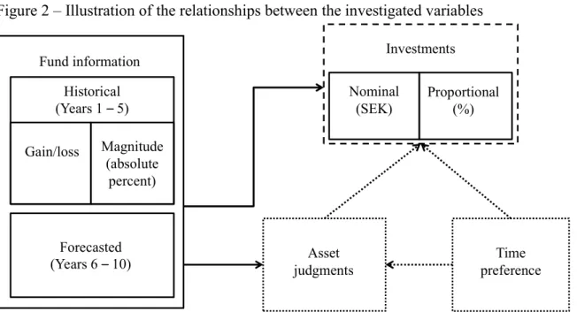
Figure 2 – Illustration of the relationships between the investigated variables
Note: Boxes with solid frame indicate variables that are manipulated by the experiment (independent), that is, the information in the investment problems and the response format. The box with the large dotted frame indicates that it is the main dependent variable (investments). The boxes with small dotted frames indicate interrelated dependent variables (asset judgments and time preference) related to the main dependent variable (investments).
2. Method
A vignette scenario was used to describe a series of fund investment tasks. The participants were randomly assigned into one of two groups, SEK and percentage. The SEK group expressed their investments as an amount of SEK (i.e. nominal investments). The percentage group
Asset judgments Investments Time preference Historical (Years 1 – 5) Gain/loss Forecasted (Years 6 – 10) Fund information Magnitude (absolute percent) Proportional (%) Nominal (SEK)
expressed their investments as a percentage of the fund assets at the time of the investment decision (i.e. proportional investments). There were no other design differences between the groups.
2.1. Participants
The participants were 87 students from Stockholm University, 22 male and 65 female. The average age was 25.78 years (SD = 7.28) with a range from 19 to 53 years. There were 47 participants in the percent condition and 40 participants in the SEK condition. Participation was rewarded with course credits. One participant misunderstood the instructions and was excluded. Another 5 participants who completed less than 14/18 of the fund investments were also excluded.1
2.2. Problems
There were 18 different fund investment problems. Each problem consisted of two consecutive 5-year accumulation periods (Figure 1). The participants’ main task was to decide how much of the assets accumulated in a fund during the first 5 years they would like to reinvest in that same fund for the second 5 years. During the first period (before the reinvestment opportunity) there was always the same annual interest rate throughout the period. The interest rates were either a gain or a loss of -20%, -10%, -1%, +1%, +10%, or +20%. During the second period (the reinvestment period, years 6 – 10) two possible outcomes were presented, one gain outcome and one loss outcome. The annual interest rate of the gain and loss outcomes were of the same numerical percentage (e.g. +10% and -10%). The percentages for the second period were ±1%, ±10%, and ±20%. The gain and loss outcomes had always equal probability (p = 0.5) of occurring (see Figure 1). The experiment included all combinations of the first period annual interest rates (6 levels) and the second period annual gain and loss interest rates (3 levels). Hence, a factorial design with 18 problems was generated.
2.3. Procedure
First, the participants signed an informed consent form to participate in the study. Then, they received information about fund asset accumulations, followed by general information about the investment problems in the experiment. Participants were not allowed to use any aids, or make notes.
Before making an investment in a fund, participants were asked to judge the fund assets accumulated from the beginning of the first year up until the end of year five. This was the only question added to the problem formulation that was used in earlier studies (Figure 1). Participants also judged the accumulated assets at the end of year 10 (i.e. second period gain and loss outcomes). Asset judgments were made with the assumption that all assets had been kept in the fund during the entire 10-year period (i.e. 100% was reinvested for years 6 – 10). After judging the asset accumulations of a fund, participants made their investment decision for that fund. The only difference between the percentage and SEK conditions was the investment response format; everything else was identical between conditions.
1 Reasons for excluding investments were (number of investments excluded): the investment was below 0% of
judged available assets (5) or above 100% (13), the judged available assets were 0 (27), the judged available assets indicated loss when there was gain (14) or gain when there was loss (27), judgment of available assets was missing (2), and judgments of available assets were above or below 5 SD of the mean (5).
After the investment problem task, participants were asked to decide how much to reinvest in fund accounts that guaranteed gain for the 5-year investment period. In this task, the assets that could be reinvested for years 6 – 10 was always SEK 10 000. The different annual interest rates for the investment period were 1%, 10% and 20%. The task was formulated similarly to the main fund investment task. The participants expressed their investments in the same format (SEK or percentage) as in the main task; see Figure 3 for an example.
This task was added to the design of the previous studies with the same fund investment problems (Gonzalez, 2017; Gonzalez % Svenson, 2014), as a measure of time preference. Figure 3 – Example of an investment problem with guaranteed gain
3. Results
The result section is divided into three subsections. Each section addresses a main topic in relation to the investment decisions. The first section addresses the effect of response format, that is, nominal (SEK) or proportional (percent) investments. The second section addresses the participants’ judgments of accumulated value after different periods of annual interest rates. The third section addresses time preference. Each section starts with aggregate analyses (group data) and then proceeds with analyses of each individual’s use of the numerical information. Group analyses are useful to find general trends while individual analyses can give a clearer picture of specific strategies. Specifically, individual analyses can find investment strategies that may be lost in group analyses. Both methods were used to cover the research question as thoroughly as possible.
To compare investment-response formats (SEK or percent) the SEK responses were converted to percentages. That is, the investment responses in SEK were divided by the judged available assets (fund value at the end of year five). Invested percentage was used as the operationalization of investment size in all analyses.
3.1. Response format and fund information 3.1.1. Group analysis
The first research question was if the response format would have an effect on investments. The participants’ average reinvested proportion of fund assets was greater in the SEK group (M = 58.33%, SD = 24.89, N = 38) compared to the percent group (M = 48.83%, SD = 25.72, N = 43), but the difference was not statistically significant.
To investigate if investments varied depending on gain and loss interest rates and response format, a mixed ANOVA was computed with the following factors; response format (percentage/SEK), sign (+/-), absolute interest rate years 1–5 (1%, 10%, 20%), interest rate of gain and loss outcomes years 6–10 (1% 10%, 20%). Note that response format was a between subjects variable while the gain and loss information were within subjects variables.
Investments were affected by the historical sign (η2 = .071) and absolute percentage (η2 = .057),
significant at the 5% level.2 The fact that the sign accounted for most of the variance (7%)
replicates the findings of Gonzalez and Svenson (2014) and Gonzalez (2017)3. However, in
contrast to these previous studies, the absolute size of the gain or loss interest rate explained as much as 6% of the variance. Investments increased when the annual gain or loss increased. No prior hypothesis was formulated regarding this finding. Therefore, the effect of absolute interest rate needs further investigation before reliable conclusions can be drawn. Average investments calculated separately for each fund can be found in appendix Table A1.
To summarize, on average, the SEK group invested 9.5% more of their accumulated assets than did the percent group, but this difference was not statistically significant. In general, investments were greater following prior gains, compared to prior losses. Investments also increased as the gains and losses increased. The effects of gain/loss and increasing gains and losses were significant on the 5% level. Forecasted outcomes were found not to affect investments.
3.1.2. Individual analyses
This study was designed to find out different investment strategies among individuals. To find out how different participants used information cues as basis for their investment decisions, the correlations between each of the investment problem cues and the size of the investments were calculated separately for each participant. For the first period (historical information) the cues were (1) sign (gain/loss), (2) annual absolute interest rate, (3) annual interest rate (sign and percentage), and (4) judged accumulated assets at the end of the first five years. For the second period, for which the investments were made, the cues were (1) annual percentage of change for the gain and loss outcomes, (2) judged gain outcome, and (3) judged loss outcome. Note that all the cues were manipulated within the experimental design (objective information) except for the judged outcomes which were judged by the participants themselves (subjective information). In the following, all correlations are Pearson’s correlations, if nothing else is stated. If a cue accounted for at least 50% of the investment variance (−0.707 ≤ r ≥ 0.707) that cue was classified as highly important for that individual. The 50% variance threshold was used so that no other unrelated variable could account for more of the investment variance, and this criterion was used by Gonzalez (2017).
Highly important cues were found only for a small amount of participants, see appendix Table A2 for a summary. This indicates a generally low reliance on specific information. However, forecasted fund development was highly important for more participants in the SEK group SEK group 7/38 (18.4%) compared to the percent group 2/43 (4.7%) (z = 1.9679, p < .05). This indicates that focusing on the nominal value of the investment, rather than the proportional value, may increase the likelihood that investors use forecasted interest rates as information to rely on for their investment decisions. It is important to note that, of the participants giving high importance to forecasted interest rates in the SEK group, three participants invested more with increasing rates, while 4 participants invested less. In the
2 There was a significant three-way interaction effect of the sign the first five years, the first period percentage and the second period percentage. This interaction explained less variance than the sign or the first period percentage F(4, 316) = 2.708, p < .05, η2 = .033. Therefore, no further interpretation will be made regarding this result.
3 We analyzed a restricted set of data with only the same stimuli as in Gonzalez (2017), that is, percentages were
equal across the entire 10 years. Only participants with complete data were used. A repeated measures ANOVA showed a significant effect of sign F(1, 59) = 5.741, p < .05, η2 = .089. No other main effects or interactions were found (second greatest η2 in the model was .008). Hence, this data replicates the findings of Gonzalez (2017).
percent group, there was one participant investing more, and one investing less, with increasing interest rates. Because greater gain and loss interest rates lead to a greater risk in this context, these findings indicate there was an equal distribution of risk averse and risk seeking individuals among the participants that gave high importance to forecasts. In other words, the participants were influenced in opposite directions by this information. This replicates findings by Gonzalez (2017) who also found that participants were influenced in the opposite direction of each other by the same information.
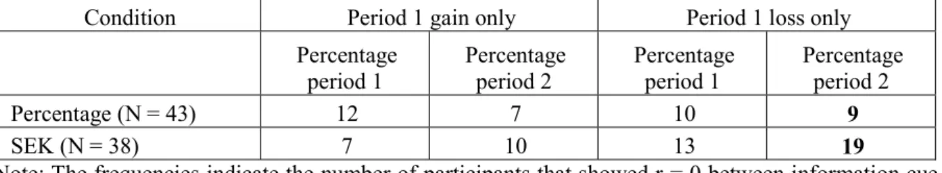
Because people tend to behave differently within the domain of gains and the domain of losses (Tversky & Kahneman, 1992), individual correlations were also separately computed for gains and losses, respectively. This analysis revealed that several participants completely ignored information (r = 0) within at least one of the gain or loss domains. Importantly, the frequency of ignoring information was different between the SEK and percentage conditions (Table 1).
Table 1 – Frequencies of participants who completely ignored information for their investment decisions in the percentage and SEK condition
Condition Period 1 gain only Period 1 loss only Percentage period 1 Percentage period 2 Percentage period 1 Percentage period 2 Percentage (N = 43) 12 7 10 9 SEK (N = 38) 7 10 13 19
Note: The frequencies indicate the number of participants that showed r = 0 between information cue and investment size. Frequencies marked in bold differ significantly, p < .01.
If there had been a previous loss, the forecasted interest rates were completely ignored to a greater extent by participants in the SEK condition 19/38 (50%) compared to the percent condition 9/43 (21%), significant on the 1% level (z = 2.745).
Four participants reinvested the same proportion in all funds. Hence, these participants ignored all variations in fund information. Investing the same proportion in all funds will be called a fixed investment strategy in the following text. Three participants reinvested all their assets in all funds; all of them where in the SEK group. Only one participant did not reinvest anything in any fund, and this participant was in the percent group. Note that to achieve the greatest EV from investments, reinvesting all assets was always the correct strategy, see equation (1). Fixed investment strategies were also analyzed separately for funds with prior gains and funds with prior losses. Maximum investments in loss funds were more common in the SEK group 6/38 (16%) compared to the percentage group 1/43 (2%), and this difference was significant on the 5% level (z = 1.983).
To summarize, the SEK group more frequently ignored forecasts for the investment period than the percent group did. The SEK group also followed a fixed investment strategy more frequently than the percent group did. This suggests that the SEK condition may have triggered a more categorical way of thinking about the different funds as good or bad to invest in. Furthermore, the SEK group tended to rely on forecasts to a greater extent than the percent group did. This indicates a greater future orientation, or focus on risks, in the SEK group, compared to the percent group.
3.2. Judgments of accumulated value
In addition to the fund information given to the participants in each problem (objective information), the participants judged the fund value at the end of year 5 and year 10. Thus, the
participants generated subjective information. This information may, or may not, be relied upon when making investments. This was the research question for the following analyses.
3.2.1. Group analysis
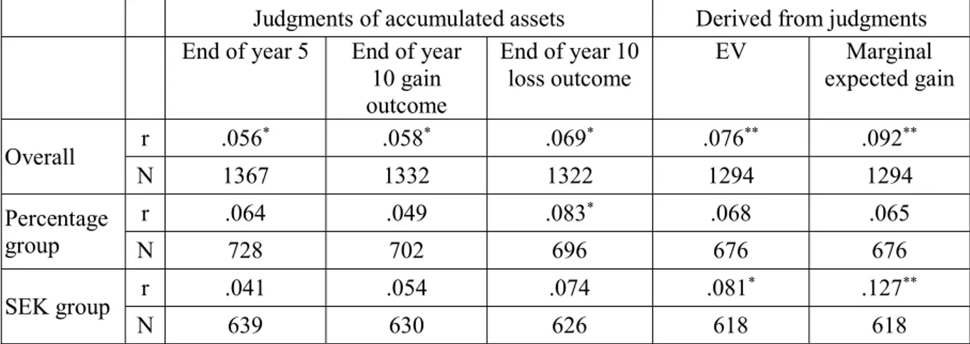
First, across all participants and fund problems, the investments were correlated with the judged assets at the end of year 5 and the gain and loss outcomes at the end of year 10. Second, investments were correlated with the subjective expected value derived from the judgments at the end of year 10 by computing (gain outcome + loss outcome)/2, and the subjective expected marginal gain (subjective expected value at the end of year 10 - judged assets at the end of year 5).4 The correlations showed that only 0.3 % to 0.8 % of the variance in the investments was
accounted for by these different judgment measures. A similar absence of correlation was found for both the SEK group and the percent group, see appendix Table A3 for details. This indicates that asset judgments were of little, if any, importance for investment decisions.
3.2.2. Individual analyses
The correlations between the different measures of judgments of accumulated assets and the investments were calculated separately for each participant. That is, the same procedure was used as for the objective information in section 3.1. If an information cue explained 50% of the variance or more (−0.707 ≤ r ≥ 0.707) that cue was classified as having high importance for that participant’s investments. The number of participants that gave high importance to an asset judgment cue (or derived cue) ranged between 0 – 6 within each condition (SEK and percent). That is, very few participants relied upon their own judgment of accumulated asset cues. Furthermore, there were no indications of reliable group differences regarding these cues. Details can be found in appendix Table A4.
3.3. Time preference
In this section the relationship between time preference, asset judgments, and investments were investigated. Asset judgments were measures of beliefs about the objective true future value while time preference is a personal preference regarding those values. Previous studies (Gonzalez, 2017; Gonzalez & Svenson, 2014) found no relationship between asset judgments and investments. To investigate investors’ future oriented thinking further, the concept of time preference was added in this study. To measure time preference, participants were asked how much of SEK 10 000 they would save in funds that guaranteed a gain (example in Figure 3). There were three different funds with the annual interest rates 1%, 10%, and 20%.5
3.3.1. Time preference and judgments of accumulated assets
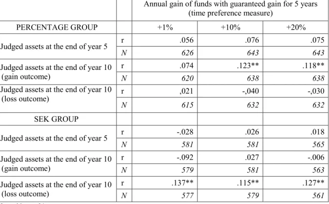
Each of the three measures of time preference were correlated with each of the judgments of asset accumulations at year 5, year 10 gain outcomes, and year 10 loss outcomes. These analyses were calculated separately for the SEK and percent group. This means that there were
4We compared asset judgments at the end of year 10 to judgments at the end of year 5. A judgment at year 10 was
excluded if, there had been a loss during years 6 – 10 and the judgment was greater than the year 5 judgment (40 excluded) and vice versa for gain outcomes (24 excluded). We also excluded judgments after 10 years of growth smaller than assets at the beginning of year 1 (SEK 10 000) after 10 years of growth (3 excluded) and judgments greater than SEK 10 000 after 10 years of decline (6 excluded). Finally, 16 judgments of accumulated assets at the end of year 10 above or below 5 SD of the mean were excluded.
5 For the time preference analysis the following were excluded, 10 participants that gave investments that were
9 correlations calculated within each group. Asset judgments shared less than 1.9% of the variance with time preference in all of the computations. The full correlation matrix can be found in appendix table A5. The low correspondence between time preference and asset judgments may indicate that the exponential growth bias is not a preference-driven bias. In other words, time preference for future assets and judgments of future assets seems to arise from different cognitive processes.
3.3.2. Time preference and investments
To find out the relationship between time preference and investments, investments across all funds were correlated with each of the three time-preference measures (guaranteed annual gain of 1%, 10% and 20%). The correlations were calculated for the SEK and percent groups separately. All correlations were positive and statistically significant at the 5% level. The shared variance between time preference and investments were between 6% and 10%, except for the 1% guaranteed gain in the SEK group (3% shared variance), see appendix Table A6 for details. It should be noted that there was a strong correlation between the funds with guaranteed annual gain of 10% and 20%, which shared 57% variance. The 1% guaranteed gain fund shared only 7% and 4% of the variance with the funds of 10% and 20% respectively.6 This indicates
that the time preference for savings with low interest rate (1%) is somewhat different than for higher interest rates (10% and 20%), and that there is not much difference when the guaranteed gain annual interest rate reaches a certain point.
To summarize, the present results indicate that time preference for saving over long horizons (five years in this study) is related between investments with risk and no risk. However, time preference is vaguely related to judgments of asset accumulations. This acts as a control of the investment data because it should be expected that a person who does not want to save their money even with guaranteed gains should not be willing to risk assets over time either. This also indicates that the exponential growth bias found in the asset judgments is not driven by time preference.
4. Discussion
The primary aim of this study was to investigate to what extent the response format (SEK or percent) can influence investment decisions made by individual investors. Response format was investigated in conjunction with how people use information about interest rates, historical and forecasted, when they make fund investments. Judgments of asset accumulations and time preference were also investigated.
Investment strategies varied in several ways between the SEK and the percent group. Forecasted gain and loss interest rates were used by more investors who expressed their investments in SEK compared to investors expressing investments as a percentage of fund assets. However, only a few participants found forecast to be highly important. Interestingly, it was also more common that SEK investors completely ignored the forecasted interest rates, and reinvested all assets after losses. A person who has lost assets in an investment may want to regain those assets to avoid it to appear as a bad investment decision. This is known as the disposition effect (Shefrin & Statman, 1985). Because the nominal capital can be perceived as more salient, the losses may have been perceived as worse for the SEK participants than for the
6 Pearson’s r between guaranteed gain investments of 10% and 20% was, r(77) = .752, p < .001, between 1% and 10% was , r(76) = .263, p < .05, and between 1% and 20% was , r(76) = .209, p = .07.
percent participants. Hence, the salience may have driven more SEK participants to keep their remaining assets in the fund in hope of regaining their lost assets.
4.1. Aggregate group analyses vs. individual analyses
In the aggregate group data analyses, average investments were greater following gains (57% reinvested) compared to losses (50% reinvested). Greater investments after gains are known as the house-money effect (Thaler & Johnson, 1990). That is, the house-money effect is the opposite of the disposition effect. Hence, the house money behavior that was indicated by the aggregate group-level analyses is in contrast to the individual-level analysis that indicated a strong disposition behavior for approximately half of the SEK condition participants. This illustrates how group averages can be misleading when interpreting data to draw conclusions about how different individuals actually act. Hence, analyzing the investment pattern of individuals can show a more detailed picture of different strategies, and a better differentiation of strategies between individuals.
It should be noted that the participants were instructed to assume their personal finances could handle an eventual loss from their fund investments. This instruction may have led some participants to consider the fund assets as money to gamble with (i.e. house money). Other studies have found a disposition effect for stocks and a house-money effect for mutual funds (Bailey et al., 2011). The disposition effect has been found to reverse (to a house-money effect) when the responsibility is shifted away from the investor (Aspara & Hoffmann, 2015). Because funds are often managed by fund managers, who can be seen as responsible for the performance of a fund, the feeling of responsibility may lower for fund investments compared to stock investments. The house-money effect is also closely related to trend chasing (Bailey et al., 2011) and a typical way of focusing too much on past performance. Hence, the participants may generally have felt low responsibility for their assets and chosen to chase trends (aggregate results). However, for a substantial amount of participants the losses became an important factor when their investments where expressed in SEK and they therefore tried to regain assets after losses (individual results).
4.2. Asset judgments and time preference
Judgments of accumulated fund asset outcomes were investigated in relation to the fund investment decisions, as well as time preference. Interestingly, judged asset outcomes have earlier been shown to have a very weak relationship with investments in the judged fund (Gonzalez, 2017; Gonzalez & Svenson, 2014). Similar results were found in the present study as well. Less than 1% of the investment variance was accounted for by the asset judgments. Because people often underestimate the accumulated change in value to a great extent (Benzion, Shachmurove &Yagil, 2004; Doerr, 2006; Timmers & Wagenaar, 1977; Wagenaar & Sagaria, 1975), judgments of accumulated value should not be used as a basis for investment decisions. Hence, it can be a good thing that investors have been found to mostly ignore their own judgments when deciding how much to invest. Interestingly, exponential growth bias has been found to correlate negatively with positive household finance behaviors (Stango & Zinman, 2009). However, these findings do not necessarily contradict the findings in the present study. In the present study, the asset outcomes of the funds that investments were made for were judged, while the Stango & Zinman (2009) study investigated judgments more generally in relation to several different behaviors. It may be that individuals who have a better general understanding of compound interest rates also have a better understanding of finance in general. This can occur without using one’s own judgment of asset outcomes as information to rely on for specific financial tasks.
To gain further understanding about asset judgments, investments and future-oriented thinking, time preference was also investigated. The time preference measure was how much a person would invest if a gain was guaranteed in five years. The task was similar to the main investment problem, but without risk of losing. Thus, it was designed to measure only the impatience for receiving their assets, that is, reluctance to wait for the assets to accumulate over the five-year investment period. Interestingly, time preference and judgments of asset outcomes barely shared any variance. This indicates that time preference is distinctly different from judgments of asset accumulation. It should be noted that participants did not judge asset accumulation for the specific time preference investment questions, which would have enabled even better separation of the concepts. Furthermore, hypothetical questions pose some risk of limited generalizability, although time preference has been found to be similar in hypothetical and real reward settings (Johnson & Bickel, 2002). To the extent that the present study investigated time preference and asset judgments, the findings support Killeen’s (2009) claim that it is the subjective utility of assets that is discounted over time, not the actual value of the assets.
Importantly, time preference correlated positively with investments, and accounted for up to 10% of the investment variance. The present study aimed to find out if time preference was a driving factor in investments, because of earlier findings that asset judgments were not. However, there was a limitation of the experimental design in that time preference was always measured last. Hence, there is a risk that the investment task influenced the time-preference task, and not the other way around. Nevertheless, if the time-preference task managed to actually capture impatience in the investors, it may be part of how much people invest when risk is involved as well. However, other factors can be more relevant for specific sets of risky fund investments. That being said, the most central finding was that the asset judgments was found to be separate from both time preference and investments.
5. Conclusion
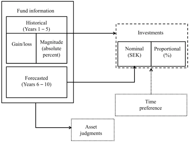
To summarize, the present study indicates that expressing investments in nominal terms, as opposed to proportional terms, may influence investors in several ways. Investors expressing nominal investments ignored more information and relied more on specific types of information. Furthermore, these investors showed a greater disposition effect, which may be an indicator of wanting to regain losses because they are more salient when thought of in nominal terms instead of proportional terms. Forecasted fund outcomes were generally not important, but when they were, it was primarily to nominal investors, and not to proportional investors. Judged asset accumulations were found to be unrelated to investment decisions, and to time preference. However, the willingness to invest in funds involving risk is related to a person’s time preference, as should be expected. An illustration of the relationship between the different factors is found in Figure 4, which is a restructured version of the introductory Figure 2.
To conclude, because different investors may behave in different ways, even if they are provided with the same information, investment advisors need to be careful when giving advice to lay people. Furthermore, the response format seems to have an effect on how people think about fund investments. Importantly, people can be affected very differently by the different formats. Hence, it may be advisable to ask investors to rethink their investment in both nominal and proportional terms. Thinking in both nominal and proportional terms may help investors towards a more complete understanding of their own decisions. This, in turn, may help investors to make investments more in line with their own preferences. A conjunction of the two response
formats can be one of many ways to keep investigating how people make long term investment decisions.
Figure 4 – Illustration of the relationships between the different variables of this experiment.
Note: On average, the participants were influenced the most by past information, and invested more following gains compared to losses. Some individuals relied heavily on the forecasted interest rates, but these were primarily found in the SEK group. Time preference was related to investments. Asset judgments were unrelated to investments as well as time preference. The solid frames indicate experimentally manipulated variables, the large dotted frame indicates the main dependent variable (investments), and the small dotted frames indicate the interrelated dependent variables (asset judgments and time preference).
Acknowledgement
This study was funded by Stockholm University, Department of Psychology. The author would like to thank Ola Svenson for valuable comments on this manuscript and Tina Sundelin for copy editing and proof reading.
References
1. Aspara, J., & Hoffmann, A. O. I. (2015). Cut your losses and let your profits run: How shifting feelings of personal responsibility reverses the disposition effect. Journal of Behavioral and Experimental Finance, 8, 18–24.
2. Bailey, W., Kumar, A., & Ng, D. (2011). Behavioral biases of mutual fund investors. Journal of Financial Economics, 102(1), 1–27. doi 10.1016/J.JFINECO.2011.05.002.
Asset judgments Investments Time preference Proportional (%) Nominal (SEK) Historical (Years 1 – 5) Gain/loss Forecasted (Years 6 – 10) Fund information Magnitude (absolute percent)
3. Benzion, U., Shachmurove, Y., & Yagil, J. (2004). Subjective discount functions - An experimental approach. Applied Financial Economics, 14(5), 299–311.
4. Choi, J. J., Laibson, D., & Madrian, B. C. (2010). Why Does the Law of One Price Fail? An Experiment on Index Mutual Funds. Review of Financial Studies, 23(4), 1405–1432. 5. Christandl, F., & Fetchenhauer, D. (2009). How laypeople and experts misperceive the
effect of economic growth. Journal of Economic Psychology, 30(3), 381–392.
6. De Bondt, W. P. M. (1993). Betting on trends: Intuitive forecasts of financial risk and return. International Journal of Forecasting, 9(3), 355–371.
7. Doerr, H. M. (2006). Examining the Tasks of Teaching When Using Students’ Mathematical Thinking. Educational Studies in Mathematics, 62(1), 3–24.
8. Eriksson, K., & Simpson, B. (2012). What do Americans know about inequality? It depends on how you ask them. Judgment & Decision Making, 7(6), 741–745.
9. Gattig, A., & Hendrickx, L. (2007). Judgmental Discounting and Environmental Risk Perception: Dimensional Similarities, Domain Differences, and Implications for Sustainability. Journal of Social Issues, 63(1), 21–39.
10. Gigerenzer, G., & Gaissmaier, W. (2011). Heuristic Decision Making. Annual Review of Psychology, 62(1), 451–482.
11. Gonzalez, N. (2017). Different investors–different decisions: On individual use of gain, loss and interest rate information. Journal of Behavioral and Experimental Finance, 15, 59–65.
12. Gonzalez, N., & Svenson, O. (2014). Growth and decline of assets: On biased judgments of asset accumulation and investment decisions. Polish Psychological Bulletin, 45(1), 29– 35.
13. Greenwood, R., & Shleifer, A. (2014). Expectations of Returns and Expected Returns. Review of Financial Studies, 27(3), 714–746.
14. Johnson, M. W., & Bickel, W. K. (2002). Within-subject comparison of real and hypothetical money rewards in delay discounting. Journal of the Experimental Analysis of Behavior, 77(2), 129–146.
15. Kahneman, D. (2003). A perspective on judgment and choice: Mapping bounded rationality. American Psychologist, 58(9), 697–720.
16. Killeen, P. R. (2009). An Additive-Utility Model of Delay Discounting. Psychological Review, 116(3), 602–619.
17. Loewenstein, G., & Prelec, D. (1992). Anomalies in Intertemporal Choice: Evidence and an Interpretation. The Quarterly Journal of Economics, 107(2), 573–597.
18. Marzilli Ericson, K. M., White, J. M., Laibson, D., & Cohen, J. D. (2015). Money Earlier or Later? Simple Heuristics Explain Intertemporal Choices Better Than Delay Discounting Does. Psychological Science.
19. McClure, S. M., Ericson, K. M., Laibson, D. I., Loewenstein, G., & Cohen, J. D. (2007). Time discounting for primary rewards. Journal of Neuroscience, 27(21), 5796–5804. 20. Mussweiler, T., & Schneller, K. (2003). “What Goes Up Must Come Down” - How Charts
Influence Decisions to Buy and Sell Stocks. Journal of Behavioral Finance, 4(3), 121– 130.
21. Newall, P. W. S., & Love, B. C. (2015). Nudging investors big and small toward better decisions. Decision, 2(4), 319–326.
22. Newall, P. W. S., & Parker, K. N. (2019). Improved Mutual Fund Investment Choice Architecture. Journal of Behavioral Finance, 20(1), 96–106.
23. Read, D. (2001). Is Time-Discounting Hyperbolic or Subadditive? Journal of Risk and Uncertainty, 23(1), 5–32.
Losers Too Long: Theory and Evidence. The Journal of Finance, 40(3), 777–790. 25. Simon, H. A. (1957). Models of man; social and rational. Oxford, England: Wiley. 26. Stango, V., & Zinman, J. (2009). Exponential growth bias and household finance. Journal
of Finance, 64(6), 2807–2849.
27. Thaler, R. H. (2016). Behavioral economics: Past, present, and future. American Economic Review, 106(7), 1577–1600.
28. Thaler, R. H., & Johnson, E. J. (1990). Gambling with the House Money and Trying to Break Even: The Effects of Prior Outcomes on Risky Choice. Management Science, 36(6), 643–660.
29. Timmers, H., & Wagenaar, W. A. (1977). Inverse statistics and misperception of exponential growth. Perception & Psychophysics, 21(6), 558–562.
30. Tversky, A., & Kahneman, D. (1992). Advances in Prospect-Theory - Cumulative Representation of Uncertainty. Journal of Risk and Uncertainty, 5(4), 297–323.
31. Wagenaar, W. A., & Sagaria, S. D. (1975). Misperception of exponential growth. Perception & Psychophysics, 18(6), 416–422.
32. Wilcox, R. T. (2003). Bargain Hunting or Star Gazing? Investors’ Preferences for Stock Mutual Funds. The Journal of Business, 76(4), 645–663.
33. Wu, L., Zeng, S., & Wu, Y. (2018). Affect Heuristic and Format Effect in Risk Perception. Social Behavior and Personality: An International Journal, 46(8), 1331–1344.
Appendix
Table A1 – Average investments in the 18 fund investment problems. Averages described separately for participants expressing their investments as SEK and as a percentage of assets
SEK GROUP PERCENT GROUP
Historical Forecasted annual interest rate (years 6 – 10) annual interest rate
(years 1 – 5) ±1% ±10% ±20% ±1% ±10% ±20% 20% 57,56 63,23 65,29 51,46 64,05 57,86 10% 69,92 58,44 58,06 53,30 58,45 48,90 1% 56,60 63,97 51,07 49,95 49,28 46,51 -1% 47,70 55,74 57,93 42,68 45,97 42,82 -10% 47,37 56,90 55,63 40,48 43,90 46,60 -20% 63,08 65,51 58,66 46,89 48,05 47,28
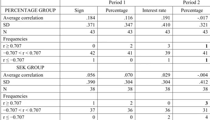
Table A2 – Descriptive statistics of participants’ individual correlation coefficients between fund information cues and investments
Period 1 Period 2
PERCENTAGE GROUP Sign Percentage Interest rate Percentage
Average correlation .184 .116 .191 -.017 SD .371 .347 .410 .321 N 43 43 43 43 Frequencies r ≥ 0.707 0 2 3 1 −0.707 < r < 0.707 42 41 39 41 r ≤ −0.707 1 0 1 1 SEK GROUP Average correlation .056 .070 .029 -.004 SD .390 .304 .304 .412 N 38 38 38 38 Frequencies r ≥ 0.707 1 2 0 3 −0.707 < r < 0.707 37 36 36 31 r ≤ −0.707 0 0 2 4
Note: Bold text indicates a significant difference, p < .05, of the proportion of participants giving high importance (r ≥ 0.707 and r ≤ −0.707) to a cue in the percent group (1+1)/43 compared to the SEK group (3+4)/38. The sign refers to only the sign (+/-). Percentage refers to the absolute annual percentage, that is, the percentage magnitude independent of sign. Interest rate refers to the annual change (including the sign +/-).
Table A3 – Pearson correlations between investments and judgments of accumulated assets, and derived expected value measures
Judgments of accumulated assets Derived from judgments End of year 5 End of year
10 gain outcome End of year 10 loss outcome EV Marginal expected gain Overall r .056 * .058* .069* .076** .092** N 1367 1332 1322 1294 1294 Percentage group r .064 .049 .083* .068 .065 N 728 702 696 676 676 SEK group r .041 .054 .074 .081 * .127** N 639 630 626 618 618
Note: Correlations were calculated across all participants and problems, * p < .05, ** p < .01. EV was derived from the asset judgments by the following calculation (judged gain outcome + judged loss outcome)/2. Marginal expected gain was derived from the asset judgments by the following calculation (EV judged - judged assets at the end of year 5).
Table A4 – Descriptive statistics of participants’ individual correlation coefficients between judgments of accumulated assets and investments
Judgments of accumulated assets Derived from judgments PERCENTAGE GROUP End of year 5 End of year 10 gain outcome End of year 10 loss outcome EV Marginal expected gain Average correlation .208 .198 .186 .201 .050 SD .393 .393 .387 .397 .294 N 43 43 43 43 43 Frequencies r ≥ 0.707 4 4 3 4 0 −0.707 < r < 0.707 37 39 39 38 43 r ≤ −0.707 2 0 1 1 0 SEK GROUP Average correlation .037 ,040 ,042 ,048 -,019 SD .426 .469 .371 .440 .312 N 38 38 38 38 38 Frequencies r ≥ 0.707 2 2 1 1 0 −0.707 < r < 0.707 34 35 36 36 37 r ≤ −0.707 2 1 1 1 1
Note: Some participants are counted as giving high importance (r ≥ 0.707 and r ≤ −0.707) in several variables because of the collinearity between the judgments. EV was derived from the asset judgments by the following calculation (judged gain outcome + judged loss outcome)/2. Marginal expected gain was derived from the asset judgments by the following calculation (EV judged - judged assets at the end of year 5).
Table A5 – Pearson correlations between investments in funds with guaranteed gain (time preference measure) and the main fund task judgments of accumulated assets after 5 years and 10 years
Annual gain of funds with guaranteed gain for 5 years (time preference measure)
PERCENTAGE GROUP +1% +10% +20%
Judged assets at the end of year 5 r .056 .076 .075
N 626 643 643
Judged assets at the end of year 10 (gain outcome)
r .074 .123** .118**
N 620 638 638
Judged assets at the end of year 10 (loss outcome)
r ,021 -,040 -,030
N 615 632 632
SEK GROUP
Judged assets at the end of year 5 r -.028 .026 .018
N 581 581 565
Judged assets at the end of year 10 (gain outcome)
r -.092 .027 -.006
N 579 581 563
Judged assets at the end of year 10 (loss outcome)
r .137** .115** .127**
N 577 579 561
Note: ** p < .01
Table A6 – Pearson correlations between investments in funds with guaranteed gain (time preference measure) and investments in funds with risk (the experiments main task)
Annual gain of funds with guaranteed gain for 5 years (time preference measure)
Investment format +1% +10% +20%
Percent Invested proportion r 0.270*** 0.310*** 0.262***
N 609 625 625
SEK Invested proportion r 0.180*** 0.259*** 0.241***
N 557 556 541