DISA W
OR
KING
P
APER
DISA
Dipartimento di Informatica
e Studi Aziendali
2009/1
Th
e Size Variance Relationship of
Business Firm Growth Rates
Massimo Riccaboni, Fabio Pammolli, Sergey V. Buldyrev,
Linda Ponta, H. Eugene Stanley
DISA
Dipartimento di Informatica
e Studi Aziendali
A bank covenants pricing model
Flavio Bazzana
DISA W
OR
KING
P
APER
2009/1
Th
e Size Variance Relationship of
Business Firm Growth Rates
Massimo Riccaboni, Fabio Pammolli, Sergey V. Buldyrev,
Linda Ponta, H. Eugene Stanley
DISA Working Papers
The series of DISA Working Papers is published by the Department of Computer and Management Sciences (Dipartimento di Informatica e Studi Aziendali DISA) of the University of Trento, Italy.
Editor
Ricardo Alberto MARQUES PEREIRA [email protected]
Managing editor
Roberto GABRIELE [email protected]
Associate editors
Flavio BAZZANA fl [email protected] Finance
Michele BERTONI [email protected] Financial and management accounting
Pier Franco CAMUSSONE [email protected] Management information systems
Luigi COLAZZO [email protected] Computer Science
Michele FEDRIZZI [email protected] Mathematics
Andrea FRANCESCONI [email protected] Public Management
Loris GAIO [email protected] Business Economics
Umberto MARTINI [email protected] Tourism management and marketing
Pier Luigi NOVI INVERARDI [email protected] Statistics
Marco ZAMARIAN [email protected] Organization theory
Technical offi cer
Paolo FURLANI [email protected]
Guidelines for authors
Papers may be written in English or Italian but authors should provide title, abstract, and keywords in both languages. Manuscripts should be submitted (in pdf format) by the corresponding author to the appropriate Associate Editor, who will ask a member of DISA for a short written review within two weeks. The revised version of the manuscript, together with the author's response to the reviewer, should again be sent to the Associate Editor for his consideration. Finally the Associate Editor sends all the material (original and fi nal version, review and response, plus his own recommendation) to the Editor, who authorizes the publication and assigns it a serial number.
The Managing Editor and the Technical Offi cer ensure that all published papers are uploaded in the international RepEc public-action database. On the other hand, it is up to the corresponding author to make direct contact with the Departmental Secretary regarding the offprint order and the research fund which it should refer to.
Ricardo Alberto MARQUES PEREIRA
Dipartimento di Informatica e Studi Aziendali Università degli Studi di Trento
The Size Variance Relationship of Business Firm Growth Rates
Massimo Riccaboni,1, 2 Fabio Pammolli,3, 2
Sergey V. Buldyrev,4 Linda Ponta,5 and H. Eugene Stanley2
1DISA, University of Trento, Via Inama 5, Trento, 38100, Italy 2Center for Polymer Studies, Boston University,
Boston, Massachusetts 02215, USA
3IMT Institute for Advanced Studies, Via S. Micheletto 3, Lucca, 55100 4Department of Physics, Yeshiva University,
500 West 185th Street, New York, NY 10033 USA
5DIFIS, Politecnico di Torino, Corso Duca degli Abruzzi 24, Torino, 10129 Italy
(Dated: April 8, 2009)
Abstract
The relationship between the size and the variance of firm growth rates is known to follow an approximate power-law behavior σ(S) ∼ S−β(S) where S is the firm size and β(S) ≈ 0.2 is an
exponent weakly dependent on S. Here we show how a model of proportional growth which treats firms as classes composed of various number of units of variable size, can explain this size-variance dependence. In general, the model predicts that β(S) must exhibit a crossover from β(0) = 0 to
β(∞) = 1/2. For a realistic set of parameters, β(S) is approximately constant and can vary in
the range from 0.14 to 0.2 depending on the average number of units in the firm. We test the model with a unique industry specific database in which firm sales are given in terms of the sum of the sales of all their products. We find that the model is consistent with the empirically observed size-variance relationship.
I. INTRODUCTION
Gibrat was probably the first who noticed the skew size distributions of economic sys-tems [1]. As a simple candidate explanation he postulated the “Law of Proportionate Ef-fect”according to which the expected value of the growth rate of a business firm is propor-tional to the current size of the firm [2]. Several models of proporpropor-tional growth have been subsequently introduced in economics [3–6]. In particular, Simon and collegues [7, 8] exam-ined a stochastic process for Bose-Einstein statistics similar to the one originally proposed by Yule [9] to explain the distribution of sizes of genera. The Simon model is a Polya Urn model in which the Gibrat’s Law is modified by incorporating an entry process of new firms. In Simon’s framework, the firms capture a sequence of many independent “opportunities” which arise over time, each of size unity, with a constant probability b that a new oppor-tunity is assigned to a new firm. Despite the Simon model builds upon the Gibrat’s Law, it leads to a skew distribution of the Yule type for the upper tail of the size distribution of firms while the limiting distribution of the Gibrat growth process is lognormal. The Law of Proportionate Effect implies that the variance σ2 of firm growth rates is independent of
size, while according to the Simon model it is inversely proportional to the size of business firms. Hymer, Pashigian and Mansfield [10, 11] noticed that the relationship between the variance of growth rate and the size of business firms is not null but decreases with increase in size of firm by a factor less than 1/K we would expect if firms were a collection of K independent subunits of approximatively equal size. In a lively debate in the mid-Sixties Simon and Mansfield [12] argued that this was probably due to common managerial influ-ences and other similarities of firm units which implies the growth rate of such components to be positive correlated. On the contrary, Hymer and Pashigian [13] maintained that larger firms are riskier than expected because of economies of scale and monopolistic power. Fol-lowing Stanley and colleagues [14] several scholars [15, 16] have recently found a non-trivial relationship between the size of the firm S and the variance σ2 of its growth rate:
σ ∼ S−β (1)
with β ≈ 0.2.
Numerous attempts have been made to explain this puzzling evidence by considering firms as collection of independent units of uneven size [14, 16–22] but existing models do
not provide a unifying explanation for the probability density functions of the growth and size of firms as well as the size variance relationship.
Thus, the scaling of the variance of firm growth rates has been considered to be a crucial unsolved problem in economics [23, 24]. Recent papers [25–29] provide a general framework for the growth and size of business firms based on the number and size distribution of their constituent parts [16–19, 30–33]. Specifically, Fu and colleagues [25] present a model of proportional growth in both the number of units and their size, drawing some general implications on the mechanisms which sustain business firm growth. According to our model, the probability density function (PDF) of the growth rates is Laplace in the center with power law tails. The PDF of the firm growth rates is markedly different from a lognormal distribution of the growth rates predicted by Gibrat and comes from a convolution of the distribution of the growth rates of constituent units and the distribution of number of units in economic systems. The model by Fu and colleagues [25] accurately predicts the shape of the size distribution and the growth distribution at any level of aggregation of economic systems. In this paper we derive the implications of the model on the size-variance relationship. In principle, the predictions of the model can be studied analytically, however due to the complexity of the resulting integrals and series which cannot be expressed in elementary functions we will rely in our study on computer simulations. The main conclusion is that the relationship between the size and the variance of growth rates is not a true power law with a single well-defined exponent β but undergoes a slow crossover from β = 0 for S → 0 to β = 1/2 for S → ∞.
II. THE MODEL
We model business firms as classes consisting of a random number of units of variable size. The number of units K is defined as in the Simon model [7]. The size of the units ξ evolves according to a geometric brownian motion or Gibrat process [1].
As in the Simon model, business firms as classes consisting of a random number of units [5, 6, 17, 30]. Firms grow by capturing new business opportunities and the probability that a new opportunity is assigned to a given firm is proportional to the number of opportunities it has already got. At each time t a new opportunity is assigned.
number of firms at time t is N(t) = N(0) + bt.
With probability 1 − b, the new opportunity is captured by an active firm α with proba-bility Pα = (1 − b)Kα(t)/t, where Kα(t) is the number of units of firm α at time t.
In the absence of the entry of new firms (b = 0) the probability distribution of the number of the units in the firms at large t, i.e. the distribution P(K) is exponential:
P (K) ≈ 1
K(t)exp(−K/K(t)), (2)
where K(t) = [n(0) + t]/N(0) is the average number of units in the classes, which linearly grows with time.
If b > 0, P (K) becomes a Yule distribution which behaves as a power law for small K:
Pnew(K) ∼ K−ϕ, (3)
where ϕ = 2 + b/(1 − b) ≥ 2, followed by the exponential decay of Eq. (2) for large K with
K(t) = [n(0) + t]1−bn(0)b/N(0) [5, 34]. This model can be generalized to the case when
the units are born at any unit of time t0 with probability θ, die with probability λ, and
in addition a new class consisting of one unit can be created with probability b0 by letting
t = t0(θ − λ + b0) and probability b = b0/(θ − λ + b0).
In the Simon model opportunities are assumed to be of unit size so that Sα(t) = Kα(t). On
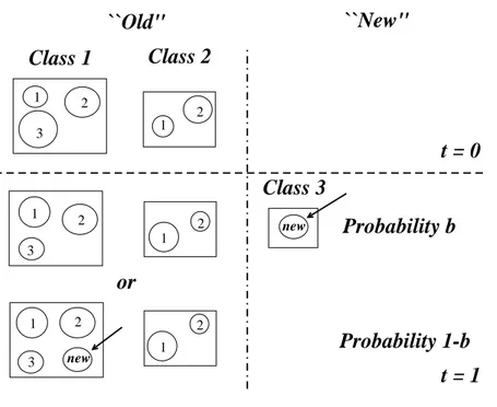
the contrary we assume that each opportunity has randomly determined but finite size. In order to capture new opportunities firms launch new products, open up new establishments, divisions or units. Each opportunity is taken up by exactly one firm and the size of the firm is measured by the sum of the sizes of the opportunities it has taken up. Fig. 1 provides a schematic representation of the model.
In the following we consider products as the relevant constituent parts of the companies and measure their size in terms of sales. The model can be applied to alternative decom-positions of economic systems in relevant subunits (i.e. plants) and measures of their sizes (i.e. number of employees).
At time t, the size of each product ξi(t) > 0 is decreased or increased by a random factor
ηi(t) > 0 so that
ξi(t) = ξi(t − 1) ηi(t), (4)
where ηi(t), the growth rate of product i, is independent random variable taken from a
distribution Pη(ηi), which has finite mean and standard deviation. We also assume that
Thus at time t a firm α has Kα(t) products of size ξi(t), i = 1, 2, ...Kα(t) so that its total
size is defined as the sum of the sales of its products Sα(t) ≡
PKα
i=1ξi(t) and its growth rate
is measured as g = log(Sα(t)/Sα(t − 1)).
The probability distribution of firm growth rates P (g) is given by
P (g) ≡
∞
X
K=1
P (K)P (g|K), (5)
where P (g|K) is the distribution of the growth rates for a firm consisting of K products. Using central limit theorem, one can show that for large K and small g, P (g|K) converge to a Gaussian distribution P (g|K) ≈ √ K √ 2πV exp µ −(g − m)2K 2V ¶ , (6)
where V and m are functions of the distributions Pξ and Pη. For the most natural
assumption of the Pure Gibrat process for the sizes of the products these distributions are lognormal: Pξ(ξi) = 1 p 2πVξ 1 ξi exp¡−(ln ξi− mξ)2/2Vξ ¢ , (7) Pη(ηi) = 1 p 2πVη 1 ηi exp¡−(ln ηi− mη)2/2Vη ¢ . (8) In this case, m = mη+ Vη/2 (9) and V ≡ Kσ2 = exp(Vξ)(exp(Vη) − 1), (10)
but for large Vξ the convergence to a Gaussian is an extremely slow process. Assuming
that the convergence is achieved, one can analytically show [25] that P (g) has similar be-havior to the Laplace distribution for small g i.e. P (g) ≈ exp(−√2|g|/√V )/√2V , while for large g P (g) has power law wings P (g) ∼ g−3 which are eventually truncated for g → ∞ by
the distribution Pη of the growth rate of a single product.
To derive the size variance relationship we must compute the conditional probability density of the growth rate P (g|S, K), of an economic system with K units and size S. For K → ∞ the conditional probability density function P (g|S, K) develops a tent shape functional form, because in the center it converges to a Gaussian distribution with the width
decreasing inverse proportionally to√K, while the tails are governed by the behavior of the
growth distribution of a single unit which remains to be wide independently of K.
We can also compute the conditional probability P (S|K), which is the convolution of K unit size distributions Pξ. In case of lognormal Pξ with a large logarithmic variance Vξ and
mean mξ, the convergence of P (S|K) to a Gaussian is very slow (see Chapter II). Since
P (S, K) = P (S|K)P (K), we can find
P (g|S) =XP (g|S, K)P (S|K)P (K), (11) where all the distributions P (g|S, K), P (S|K), P (K) can be found from the parameters of the model. P (S|K) has a sharp maximum near S = SK ≡ Kµξ, where µξ = exp(mξ+ Vξ/2)
is the mean of the lognormal distribution of the unit sizes. Conversely, P (S|K) as function of K has a sharp maximum near KS = S/µξ. For the values of S such that P (KS) >> 0,
P (g|S) ≈ P (g|KS), because P (S|K) serves as a δ(K − KS) so that only terms with K ≈ KS
make a dominant contribution to the sum of Eq. (11). Accordingly, one can approximate
P (g|S) by P (g|KS) and σ(S) by σ(KS). However, all firms with S < S1 = µξ consist
essentially of only one unit and thus
σ(S) =pVη (12)
for S < µξ. For large S if P (KS) > 0
σ(S) = σ(KS) = p V /KS = exp(3Vξ/4 + mξ/2) p exp(Vη) − 1 √ S (13)
where mη and Vη are the logarithmic mean and variance of the unit growth distributions Pη
and V = exp(Vξ)[exp(Vη) − 1]. Thus one expects to have a crossover from β = 0 for S < µξ
to β = 1/2 for S >> S∗, where
S∗ = exp(3Vξ/2 + mξ)(exp(Vη) − 1)/Vη (14)
is the value of S for which Eq.(12) and Eq.(13) give the same value of σ(S). Note that for small Vη < 1, S∗ ≈ exp(3Vξ/2 + mξ). The range of crossover extends from S1 to S∗, with S∗/S
1 = exp(Vξ) → ∞ for Vξ → ∞. Thus in the double logarithmic plot of σ vs. S one can
find a wide region in which the slope β slowly vary from 0 to 1/2 (β ≈ 0.2) in agreement with many empirical observations.
The crossover to β = 1/2 will be observed only if K∗ = S∗/µ
ξ = exp(Vξ) is such that
P (K∗) is significantly larger than zero. For the distribution P (K) with a sharp exponential
cutoff K = K0, the crossover will be observed only if K0 >> exp(Vξ).
Two scenarios are possible for S > S0 = K0µξ. In the first, there will be no economic
system with S >> S0. In the second, if the distribution of the size of units Pξ is very broad,
large economic systems can exist just because the size of a unit can be larger than S0. In
this case exceptionally large systems might consist of one extremely large unit ξmax, whose
fluctuations dominate the fluctuations of the entire system.
One can introduce the effective number of units in a system Ke = S/ξmax, where ξmax
is the largest unit of the system. If Ke < 2, we would expect that σ(S) will again become
equal to its value for small S given by Eq. (12), which means that under certain conditions
σ(S) will start to increase for very large economic systems and eventually becomes the same
as for small ones.
Whether such a scenario is possible depends on the complex interplay of Vξ and P (K).
The crossover to β = 1/2 will be seen only if P (K > K∗) > P (ξ > S∗) which means that
such large systems predominantly consist of a large number of units. Taking into account the equation of Pξ, one can see that P (ξ > S∗) ∼ exp(−9/8Vξ).
On the one hand, for an exponential P (K), this implies that
exp(− exp(Vξ)/K0) > exp(−9/8Vξ) (15)
or
Vξ > 8 exp(Vξ)/(9K0). (16)
This condition is easily violated if Vξ >> ln K0. Thus for the distributions P (K) with
exponential cut-off we will never see the crossover to β = 1/2 if Vξ >> ln K0.
On the other hand, for a power law distribution P (K) ∼ K−φ, the condition of the
crossover becomes exp(Vξ)1−φ > exp(−9/8Vξ), or (φ − 1)Vξ < 9/8Vξ which is rigorously
satisfied for
φ < 17/8 (17)
expect a crossover to β = 1/2 for large S and significantly large number N of economic entities in the data set: NP (K∗) > 1. The sharpness of the crossover mostly depends on V
ξ.
For power law distributions we expect a sharper crossover than for exponential ones because the majority of the economic systems in a power law distribution have a small number of units K, and hence β = 0 almost up to S∗, the size at which the crossover is observed. For
exponential distributions we expect a slow crossover which is interrupted if Vξ is comparable
to ln K0. For S >> S1 this crossover is well represented by the behavior of σ(KS).
We confirm these heuristic arguments by means of computer simulations. Figure 9 shows the behavior of σ(S) for the exponential distribution P (K) = exp(−K/hKi)/hKi and log-normal Pξ and Pη. We show the results for K0 = 1, 10, 100, 1000, 10000 and Vξ = 1, 5, 10.
The graphs σ(KS) and the asymptote given by Eq.(13) are also given to illustrate our
the-oretical considerations. One can see that for Vξ = 1, σ(S) almost perfectly follows σ(KS)
even for hKi = 10. However for Vξ = 5, the deviations become large and σ(S) converges to
σ(KS) only for hKi > 100. For Vξ = 10 the convergence is never achieved.
Figures 2 and 6 illustrate the importance of the effective number of units Ke. When KS
becomes larger than K0, σ(S) starts to follow σ(Ke). Accordingly, for very large economic
systems σ(S) becomes almost the same as for small ones. The maximal negative value of the slope βmax of the double logarithmic graphs presented in Fig. 2(a) correspond to
the inflection points of these graphs, and can be identified as approximate values of β for different values of K0. One can see that βmax increases as K0 increases from a small value
close to 0 for K0 = 10 to a value close to 1/2 for K0 = 105 in agreement with the predictions
of the central limit theorem.
To further explore the effect of the P (K) on the size-variance relationship we select P (K) to be a pure power law P (K) ∼ K−2 [Fig. 3(a)]. Moreover, we consider a realistic P (K)
where K is the number of products by firms in the pharmaceutical industry [Fig. 3(b)]. As we have seen in Chapter II, this distribution can be well approximated by a Yule distribution with φ = 2 and an exponential cut-off for large K. Figure 3 shows that, for a scale-free power-law distribution P (K), in which the majority of firms are comprised of small number of units, but there is a significant fractions firms comprised of an arbitrary large number of units, the size variance relationship depicts a steep crossover from σ = pVη given by
Eq. (12) for small S to σ = pV /KS given by Eq. (13) for large S, for any value of Vξ
As we see, the size-variance relationship of economic systems σ(S) can be well approxi-mated by the behavior of σ(KS) [Fig 2(a)]. It was shown in Buldyrev (2007) that, for realistic
Vξ, σ2(K) can be approximated in a wide range of K as σ(K) ∼ K−β with β ≈ 0.2, which
eventually crosses over to K−1/2 for large K. In other words, one can write σ(K) ∼ K−β(K)
where β(K), defined as the slope of σ(K) on a double logarithmic plot, increases from a small value dependent on Vξ at small K to 1/2 for K → ∞. Accordingly, one can expect
the same behavior for σ(S) for KS < K0.
As KS approaches K0, σ(S) starts to deviate from σ(KS) in the upward direction. This
results in the decrease of the slope β(S) as S → ∞ and one may not see the crossover to
β = 1/2. Instead, in a quite large range of parameters β can have an approximately constant
value between 0 and 1/2.
Thus it would be desirable to derive an exact analytical expression for σ(K) in case of lognormal and independent Pξ and Pη. Using the fact that the n-th moment of the lognormal
distribution Px(x) = 1 √ 2πVx 1 x exp ¡ −(ln xi− mx)2/2Vx ¢ , (18) is equal to µn,x ≡ hxni = exp(nmx+ n2Vx/2) (19)
we can make an expansion of a logarithmic growth rate in inverse powers of K:
g = ln PK i=1ξiηi PK i=1ξi = ln µ1,η + ln µ 1 + A K(1 + B/K) ¶ = mη + Vη 2 + A(1 − B/K + B2/K2...) K − A2(1 − B/K + B2/K2...)2 2K2 + ... = mη + Vη 2 + A K − AB + A2/2 K2 + O(K −3) where A = PK i=1ξi(ηi− µ1,η) µ1,ηµ1,ξ (20) B = PK i=1ξi− µ1,ξ µ1,ξ . (21)
Using the assumptions that ξi, and ηi are independent: hξiηii = hξiihηii, hηiηji = hηiihηji,
with a = exp(Vξ) and b = exp(Vη). Thus µ = hgi = ∞ X n=0 mn Kn σ2 = hg2i − µ2 = ∞ X n=1 Vn Kn, (22) where m0 = mη + Vη/2, m1 = −C/2, V1 = C, V2 = C[a(5b + 1)/2 − 1 − a2b(b + 1)].
The higher terms involve terms like hAni/Kn, which will become sums of various products
hξk
i(ηi − µ1,η)ki, where 2 ≤ k ≤ n. The contribution from k = n has exactly K terms of µn,ξµ−n1,ξ Pn j=0µj,ηµ−j1,η(−1)n−j ¡j n ¢
with µj,xµ−j1,x = exp(Vxj(j − 1)/2). Thus there are
contri-butions to mn and Vn which grow as (ab)n(n+1)/2 with ab > 1, which is faster than the n-th
power of any λ > 0. Thus the radius of convergence of the expansions (22) is equal to zero, and these expansions have only a formal asymptotic meaning for K → ∞. However, these expansions are useful since they demonstrate that µ and σ do not depend on mη and mξ
except for the leading term in µ: m0 = mη+ Vη/2.
Not being able to derive close-form expressions for σ, we perform extensive computer simulations, where ξ and η are independent random variables taken from lognormal distri-butions Pξ and Pη with different Vξ and Vη. The numerical results (Fig. 4) suggest that
ln σ2(K)K/C ≈ F
σ[ln(K) − f (Vξ, Vη)] , (23)
where Fσ(z) is a universal scaling function describing a crossover from Fσ(z) → 0 for z → ∞
to Fσ(z)/z → 1 for z → −∞ and f (Vξ, Vη) ≈ fξ(Vξ) + f η(Vη) are functions of Vξ and Vη
which have linear asymptotes for Vξ → ∞ and Vη → ∞ [Fig. 4(b)].
Accordingly, we can try to define β(z) = (1−dFσ/dz)/2 [Fig. 5 (a)]. The main curve β(z)
can be approximated by an inverse linear function of z, when z → −∞ and by a stretched exponential as it approaches the asymptotic value 1/2 for z → +∞. The particular analytical shapes for these asymptotes are not known and derived solely from least square fitting of the numerical data. The scaling for β(z) is only approximate with significant deviations from a universal curve for small K. The minimal value for β practically does not depend on Vη
and is approximately inverse proportional to a linear function of Vξ:
βmin =
1
pVξ+ q
(24) where p ≈ 0.54 and q ≈ 2.66 are universal values [Fig. 5(b)]. This finding is significant for our study, since it indicates that near its minimum, β(K) has a region of approximate
constancy with the value βmin between 0.14 and 0.2 for Vξ between 4 and 8. These values
of Vξ are quite realistic and correspond to the distribution of unit sizes spanning over from
roughly two to three orders of magnitude (68% of all units), which is the case in the majority in economic and ecological systems. Thus our study provides a reasonable explanation for the abundance of value of β ≈ 0.2.
The above analysis shows that σ(S) is not a true power-law function, but undergoes a crossover from β = βmin(Vξ) for small economic systems to β = 1/2 for large ones. However
this crossover is expected only for very broad distributions P (K). If it is very unlikely to find an economic complex with K > K0, σ(S) will start to grow for S > K0µξ. Empirical
data do not show such an increase (Fig. 7), because in reality there are few giant entities which rely on few extremely large units. These entities are extremely volatile and hence unstable. Therefore for real data we do see neither a crossover to β = 1/2 nor an increase of σ for large economic systems.
III. THE EMPIRICAL EVIDENCE
Since the size variance relationship depends on the partition of firms into their constituent components, to properly test our model one must decompose an economic system into parts. In this section we analyze the pharmaceutical industry database which covers the whole size distribution for products and firms and monitors flows of entry and exit at every level of aggregation. Products are classified by companies, markets and international brand names, with different distributions P (K) with hKi = K0 ranging from 5.8 for international
products to almost 1,600 for markets [Tab. I]. If firms have on average K0 products and Vξ << ln K0, the scaling variable z = K0 is positive and we expect β → 1/2.On the
contrary, if Vξ >> ln K0, z < 0 and we expect β → 0. These considerations work only for a
broad distribution of P (K) with mild skewness such as an exponential distribution. At the opposite extreme, if all companies have the same number of products, the distribution of S is narrowly concentrated near the most probable value S0 = µξK and there is no reason to
define β(S). Only very rarely S >> S0, due to a low probability of observing an extremely
large product which dominates the fluctuation of a firm. Such a firm is more volatile than other firms of equal size. This would imply negative β. If P (K) is power law distributed, there is a wide range of values of K, so that there are always firms for which ln K >> Vξ
and we can expect a slow crossover from β = 0 for small firms to β = 1/2 for large firms, so that for a wide range of empirically plausible Vξ, β is far form 1/2 and statistically different
from 0. The estimated value of the size-variance scaling coefficient β goes form 0.123 for products to 0.243 for therapeutic markets with companies in the middle (0.188) [Tab. I and Fig. 6].
Our model relies upon general assumptions of independence of the growth of economic entities from each other and from the number of units K. However, these assumptions could be violated and at least three alternative explanations must be analyzed:
1. Size dependence. The probability that an active firm captures a new market oppor-tunity is more or less than proportional to its current size. In particular, there could be a positive relationship between the number of products of firm α (Kα) and the
size (ξi(α)) and growth (ηi(α)) of its component parts due to monopolistic effects and
economies of scale and scope. If large and small companies do not get access to the same distribution of market opportunities, large firms can be riskier than small firms simply because they tend to capture bigger opportunities.
2. Units interdependence. The growth processes of the consituent parts of a firm are not independent. One could expect product growth rates to be positively correlated at the level of firm portfolios, due to product similarities and common management, and negatively correlated at the level of relevant markets, due to substitution effects and competition. Based on these arguments, one would predict large companies to be less risky than small companies because their product portfolios tend to be more diversified.
3. Time dependence. The growth of firms constituent units does not follow a pure Gibrat process due to serial auto-correlation and lifecycles. Young products and firms are supposed to be more volatile then predicted by the Gibrat’s Law due to learning effects. If large firms are older and have more mature products, they should be less risky than small firms. On the contrary, ageing and obsolescence would imply that incumbent firms are more unstable than newcomers.
The number of products of a firm and their average size defined as hξ(K)i = h1
K
PK
i=1ξii,
where hi indicates averaging over all companies with K products, has an approximate power law dependence hξ(K)i ∼ Kγ, where γ = 0.38.
The mean correlation coefficient of product growth rates at the firm level hρ(K)i shows an approximate power law dependence hρ(K)i ∼ Kζ, where ζ = −0.36.
Since larger firms are composed by bigger products and are more diversified than small firms the two effects compensate each other. Thus if products are randomly reassigned to companies, the size variance relationship will not change.
As for the time dependence hypothesis, despite there are some departures from a Gibrat process at the product level (Fig. 11) due to lifecycles and seasonal effects, they are too weak to account for the size variance relationship. Moreover asynchronous product lifecycles are washed out upon aggregation.
To discriminate among different plausible explanaitons we run a set of experiments in which we keep the real P (K) and randomly reassign products to firms. In the first simulation we randomly reassign products by keeping the real world relationship between the size, ξ, and growth, η, of products. In the second simulation we reassign also η. Finally in the last simulation we generate elementary units according to a geometric brownian motion (Gibrat process) with empirically estimated values of the mean and variance of ξ and η. Tab. I summarizes the results of our simulations.
The first simulation allows us to check for the size dependence and unit interdepence hypotheses by randomly reassigning elementary units to firms and markets. In doing that, we keep the number of the products in each class and the history of the fluctuation of each product sales unchanged. As for the size dependence, our analysis shows that there is indeed strong correlation between the number of products in the company and their average size defined as hξ(K)i = h 1 K K X i=1 ξii, (25)
where hi indicates averaging over all companies with K products. We observe an ap-proximate power law dependence hξ(K)i ∼ Kγ, where γ = 0.38. If this would be a true
asymptotic power law holding for K → ∞ than the average size of the company of K prod-ucts would be proportional to ξ(K)K ∼ K1+γ. Accordingly, the average number of products
in the company of size S would scale as K0(S) ∼ S1/(1+γ) and consequently due to central
limit theorem β = 1/(2 + 2γ). In our data base, this would mean that the asymptotic value of β = 0.36. Similar logic was used to explain β in [15, 19]. Another effect of random redis-tribution of units will be the removal of possible correlations among ηi in a single firm (unit
interdependence). Removal of positive correlations would decrease β, while removal of neg-ative correlations would increase β. The mean correlation coefficient of the product growth rates at the firm level hρ(K)i also has an approximate power law dependence hρ(K)i ∼ Kζ,
where ζ = −0.36. Since larger firms have bigger products and are more diversified than small firms the size dependence and unit interdepencence cancel out and β practically does not change if products are randomly reassigned to firms.
N K0 β1 β1∗ β2∗ β3∗
Markets 574 1,596.9 0.243 0.213 0.232 0.221 Firms 7,184 127.5 0.188 0.196 0.125 0.127 International Products 189,302 5.8 0.151 0.175 0.038 0.020 All Products 916,036 – 0.123 0.123 0 0
TABLE I: The size-variance relationship σ(S) ∼ S−β(S): estimated values of β and simulation
results β∗at different levels of aggregations from products to markets. In simulation 1 (β1∗) products are randomly reassigned to firms and markets. In simulation 2 (β∗
2) the growth rates of products
are reassigned too. In simulation 3 (β3∗) we reproduce our model with real P (K) and estimated values of mξ= 7.58 and Vξ = 2.10.
To control the effect of time dependence, we keep the sizes of products ξiand their number
Kα at year t for each firm α unchanged, so St=
PKα
i=1ξi is the same as in the empirical data.
However, to compute the sales of a firm in the following year eSt+1=
PKα
i=1ξi0, we assume that
ξ0
i = ξiηi, where ηi is an annual growth rate of a randomly selected product. The surrogate
growth rate eg = lnSet+1
St obtained in this way does not display any size-variance relationship
at the level of products (β∗
2 = 0). However, we still observe a size variance relationship at
higher levels of aggregation. This test demonstrates that 1/3 of the size variance relationship depends on the growth process at the level of elementary units which is not a pure Gibrat process. However, asynchronous product lifecycles are washed out upon aggregation and there is a persistent size-variance relationship which is not due to product auto-correlation.
Finally we reproduced our model with the empirically observed P (K) and the estimated moments of the lognormal distribution of products (mξ = 7.58, Vξ = 4.41). We generate
N random products according to our model (Gibrat process) with the empirically observed
level of Vξ and mξ. As we can see in Tab. I, our model closely reproduce the values of β
at any level of aggregation. We conclude that a model of proportional growth in both the number and the size of economic units correctly predicts the size-variance relationship and the way it scales under aggregation.
The variance of the size of the constituent units of the firm Vξand the distribution of units
into firms are both relevant to explain the size variance relationship of firm growth rates. Simulations results in Fig. 7 reveal that if elementary units are of the same size (Vξ = 0)
the central limit theorem will work properly and β ≈ 1/2. As predicted by our model, by increasing the value of Vξ we observe at any level of aggregation the crossover of β form 1/2
to 0. The crossover is faster at the level of markets than at the level of products due to the higher average number of units per class K0. However, in real world settings the central
limit theorem never applies because firms have a small number of components of variable size (Vξ > 0). For empirically plausible values of Vξ and K0 β ≈ 0.2.
IV. DISCUSSION
Firms grow over time as the economic system expands and new investment opportunities become available. To capture new business opportunities firms open new plants and launch new products, but the revenues and return to the investments are uncertain. If revenues were independent random variables drawn from a Gaussian distribution with mean me and
variance Ve one should expect that the standard deviation of the sales growth rate of a firm
with K products will be σ(S) ∼ S−β(S) with β = 1/2 and S = m
eK. On the contrary, if the
size of business opportunities is given by a geometric brownian motion (Gibrat’s process) and revenues are independent random variables drawn from a lognormal distribution with mean
mξ and variance Vξ the central limit theorem does not work effectively and β(S) exhibits a
crossover from β = 0 for S → 0 to β = 1/2 for S → ∞. For realistic distributions of the number and size of business opportunities, β(S) is approximately constant, as it varies in the range from 0.14 to 0.2 depending on the average number of units in the firm K0 and
expected to be riskier than the sum of S firms of size 1, even in the case of constant returns to scale and independent business opportunities.
[1] Gibrat R (1931) Les in´egalit´es ´economiques (Librairie du Recueil Sirey, Paris). [2] Sutton J (1997) Gibrat’s legacy. J Econ Lit 35:40-59.
[3] Kalecki M (1945) On the Gibrat distribution. Econometrica 13:161-170.
[4] Steindl J (1965) Random processes and the growth of firms: a study of the Pareto law (Griffin, London).
[5] Ijiri Y, Simon H A (1977) Skew distributions and the sizes of business firms (North-Holland Pub. Co., Amsterdam).
[6] Sutton J, (1998) Technology and market structure: theory and history (MIT Press, Cambridge, MA.).
[7] Simon H A (1955) On a class of skew distribution functions. Biometrika 42:425-440.
[8] Ijiri Y, Simon H A (1975) Some distributions associated with Bose-Einstein statistics. Proc
Natl Acad Sci USA 72:1654-1657.
[9] Yule U (1925) A mathematical theory of evolution, based on the conclusions of Dr. J. C. Willis. Philos Trans R Soc London B 213:21-87.
[10] Hymer, S. & Pashigian, P. (1962) Firm size and rate of growth J. of Pol. Econ. 70:556-569. [11] Mansfield, E. (1962) Entry, Gibrat’s law, innovation, and the growth of firms Amer. Econ. Rev.
52:1023-1051.
[12] Simon, H. A. (1964) Comment: Firm size and rate of growth J. of Pol. Econ. 72:81-82. [13] Hymer, S. & Pashigian, P. (1964) Firm size and rate of growth: Reply J. of Pol. Econ.
72:83-84.
[14] Stanley M H R, Amaral L A N, Buldyrev S V, Havlin S, Leschhorn H, Maass P, Salinger M A, Stanley H E (1996) Scaling behavior in the growth of companies. Nature 379:804-806.
[15] Bottazzi G, Dosi G, Lippi M, Pammolli F & Riccaboni M (2001) Innovation and corporate growth in the evolution of the drug industry. Int J Ind Org 19:1161-1187.
[16] Sutton J (2002) The variance of firm growth rates: the ‘scaling’ puzzle. Physica A 312:577–590. [17] De Fabritiis G D, Pammolli F, Riccaboni M (2003) On size and growth of business firms.
[18] Buldyrev S V, Amaral L A N, Havlin S, Leschhorn H, Maass P, Salinger M A, Stanley H E, Stanley M H R (1997) Scaling behavior in economics: II. modeling of company growth. J Phys I
France 7:635–650.
[19] Amaral L A N, Buldyrev S V, Havlin S, Leschhorn H, Maass P, Salinger M A, Stanley H E, Stanley M H R (1997) Scaling behavior in economics: I. empirical results for company growth.
J Phys I France 7:621–633.
[20] Aoki M, Yoshikawa H (2007) Reconstructing macroeconomics: a perspective from
statisti-cal physics and combinatorial stochastic processes (Cambridge University Press, Cambridge,
MA.).
[21] Axtell R (2006) Firm sizes: facts, formulae and fantasies (CSED Working Paper 44).
[22] Klepper S, Thompson P (2006) Submarkets and the evolution of market structure RAND
J Econ 37:861–886.
[23] Gabaix X (1999) Zipf’s law for cities: an explanation. Quar J Econ 114:739–767.
[24] Armstrong M, Porter R H (2007) Handbook of industrial organization, Vol. III (North Holland, Amsterdam).
[25] Fu D, Pammolli F, Buldyrev S V, Riccaboni M, Matia K, Yamasaki K, Stanley H E (2005) The growth of business firms: theoretical framework and empirical evidence. Proc Natl Acad
Sci USA 102:18801.
[26] Buldyrev S V, Growiec G, Pammolli F, Riccaboni M, Stanley H E (2008) The growth of business firms: facts and theory. J Eu Econ Ass 5:574-584.
[27] Growiec G, Pammolli F, Riccaboni M, Stanley H E (2008) On the size distribution of business firms. Econ Lett 98:207-212.
[28] Buldyrev S V, Pammolli F, Riccaboni M, Yamasaki K, Fu D, Matia K, Stanley H E (2007) A generalized preferential attachment model for business firms growth rates - II. Mathematical treatment. Europ Phys J B 57:131-138.
[29] Pammolli F, Fu D, Buldyrev S V, Riccaboni M, Matia K, Yamasaki K, Stanley H E (2007) A generalized preferential attachment model for business firms growth rates - I. Empirical evidence Europ Phys J B 57:127-130.
[30] Amaral L A N, Buldyrev S V, Havlin S, Salinger M A, Stanley H E (1998) Power law scaling for a system of interacting units with complex internal structure. Phys Rev Lett 80:1385–1388. [31] Takayasu H, Okuyama K (1998) Country dependence on company size distributions and a
numerical model based on competition and cooperation. Fractals 6:67–79.
[32] Canning D, Amaral L A N, Lee Y, Meyer M, Stanley H E (1998) Scaling the volatility of GDP growth rates. Econ Lett 60:335–341.
[33] Buldyrev S V, Dokholyan N V, Erramilli S, Hong M, Kim J Y, Malescio G, Stanley H E (2003) Hierarchy in social organization. Physica A 330:653–659.
[34] Yamasaki K, Matia K, Buldyrev S V, Fu D, Pammolli F, Riccaboni M, Stanley H E (2006) Preferential attachment and growth dynamics in complex systems. Phys Rev E 74:035103.
t = 0
t = 1
1 2 3or
1 2 3 1 2 1 2 1 2 3 2 1 new``Old"
``New"
Probability b
Probability 1-b
Class 1
Class 2
Class 3
newFIG. 1: Schematic representation of the model of proportional growth. At time t = 0, there are N (0) = 2 classes (¤) and n(0) = 5 units (°) (Assumption A1). The area of each circle is proportional to the size ξ of the unit, and the size of each class is the sum of the areas of its constituent units (see Assumption B1). At the next time step, t = 1, a new unit is created (Assumption A2). With probability b the new unit is assigned to a new class (class 3 in this example) (Assumption A3). With probability 1 − b the new unit is assigned to an existing class with probability proportional to the number of units in the class (Assumption A4). In this example, a new unit is assigned to class 1 with probability 3/5 or to class 2 with probability 2/5. Finally, at each time step, each circle i grows or shrinks by a random factor ηi (Assumption B2).
100 101 102 103 104 105 106 107 108 109 S 10-2 10-1 100 σ <K>=101, βmax= 0.09 <K>=102, βmax= 0.11 <K>=103, βmax= 0.19 <K>=104, βmax= 0.29 <K>=105, βmax= 0.40 σ(<K>), S=µξ<K> (a) 100 101 102 103 104 105 106 107 108 109 S 100 101 102 103 K e <K>=101 <K>=102 <K>=103 <K>=104 <K>=105 S=<K>µξ (b)
FIG. 2: (a) Simulation results for σ(S) according to Eq. (11) for exponential P (K) = exp(−K/K0)/K0 with K0 = 10, 102, 103, 104, 105 and lognormal Pξ and Pη with Vξ = 5.13, mξ =
3.44, Vη = 0.36, µη = 0.016 computed for the pharmaceutical database. One can see that, for small
enough S and for different K0, σ(S) follows a universal curve which can be well approximated with
σ(KS), with KS = S/µξ ≈ S/405. For KS > K0, σ(S) departs from the universal behavior and starts to increase. This increase can be explained by the decrease of the effective number of units
Ke(S) for the extremely large firms. The maximal negative slope βmaxincreases as K0 increases in
agreement with the predictions of the central limit theorem. (b) One can see, that Ke(S) reaches
its maximum around S ≈ Kµξ. The positions of maxima in Ke(S) coincide with the positions of minima in σ(S).
10-2 100 102 104 106 108 S 10-3 10-2 10-1 100 σ Vξ=1 Vξ=5 Vξ=10 (a) 10-2 100 102 104 106 S 10-2 10-1 100 σ Vξ=1 Vξ=5 Vξ=10 (c)
FIG. 3: Size variance relationship σ(S) for various Vξ with P (K) ∼ K−2 (a) and real P (K) (b).A
sharp crossover from β = 0 to β = 1/2 is seen for the power law distribution even for large values of Vξ. In case of real P (K) one can see a wide crossover regions in which σ(S) can be approximated
by a power-law relationship with 0 < β < 1/2. Note that the slope of the graphs (β) decreases with the increase of Vξ. The graphs of β(KS) and their asymptotes are also shown with squares
and circles, respectively.
-15 -10 -5 0 5 10 15 ln(K)-f(Vξ,Vη) -12 -10 -8 -6 -4 -2 0 ln( σ K/V) Vη=1,Vξ=1 Vη=1,Vξ=5 Vη=1,Vξ=10 Vη=0.5,Vξ=1 Vη=0.5,Vξ=5 Vη=0.5,Vξ=10 (a) 0 2 4 6 8 10 Vξ 0 5 10 15 f(V ξ ,V η )-f η (V η ) (b) Vη=1.0 Vη=0.5 Vη=0.1 0 0,5 1 Vη 0 0,5 1 f η (V η )
FIG. 4: (a) Simulation results for σ2(K) in case of lognormal P
ξ and Pη and different Vξ and Vη
plotted on a universal scaling plot as a functions of scaling variable z = ln(K) − f (Vξ, Vη). (b) The shift function f (Vξ, Vη). The graph shows that f (Vξ, Vη) ≈ fξ(Vξ) + fη(Vη) Both fξ(Vξ) and fη(Vη)
-15 -10 -5 0 5 10 15 ln(K)-f(Vξ,Vη) 0 0.1 0.2 0.3 0.4 0.5 β Vη=1,Vξ=1 Vη=1,Vξ=5 Vη=1,Vξ=10 Vη=0.5,Vξ=1 Vη=0.5,Vξ=5 Vη=0.5,Vξ=10 1/(3.1-0.44z) 0.5-1.8e-0.75z (a) 0 2 4 6 8 10 Vx 0.1 0.2 0.3 0.4 β min Vη=1.0 Vη=0.5 Vη=0.1 y=1/(2.66+0.54x) (b)
FIG. 5: (a) The effective exponent β(z) obtained by differentiation of σ2(z) plotted in Fig. 4 (a). Solid lines indicate least square fits for the left and right asymptotes. The graph shows significant deviations of β(K, Vξ, Vη) from a universal function β(z) for small K, where β(K) develops minima.
(b) The dependence of the minimal value of βmin on Vξ. One can see that this value practically
100 101 102 103 104 105 106 107 108 109 1010
S
10-2 10-1 100σ
1/K
eFIG. 6: The standard error of firm growth rates (σ) (circles), and the share of the largest products (1/Ke) (squares) versus the size of the firm (S). As predicted by our model for S < S1 = µξ≈ 3.44,
β ≈ 0. For S > S1 β increases but never reaches 1/2 due to the slow grow of the effective number
of products (Ke). The flattering of the upper tail is due to some large companies with unusually
0
5
10
15
20
25
V
ξ0
0.1
0.2
0.3
0.4
0.5
β
Products
Firms
Markets
FIG. 7: The scaling of the size-variance relationship as a function of Vξ. β decays rapidly from 1/2
to 0 for Vξ → ∞. In the simulation we keep the real P (K) for products, companies and markets
and assign products drawn from a lognormal distribution with the empirically observed mean mξ
−3 −2 −1 0 1 2 3
g
10−5 10−4 10−3 10−2 10−1 100 101P(g|S,K)
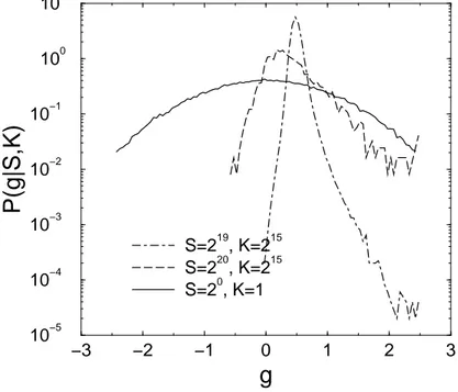
S=219, K=215 S=220, K=215 S=20, K=1FIG. 8: Simulation results for the conditional growth rate distribution P (g|S, K) for the case of lognormal Pξ and Pη, with Vξ = 6, Vη = 1 and mξ = mη = 0. For K = 1 the distribution is
perfectly Gaussian with Vη = 1 and mη = 0. However for large K the distribution develops a
tent-shape form with the central part close to a Gaussian with mean m = 1/2 as predicted by Eq. (9). The vast majority of firms (99.7%) have sizes in the vicinity of Kµξ which for K = 215 and
µξ = exp(mξ+ Vξ/2) = 20.1 belongs to the bin [219, 220] and only 0.25% of firms belong to the
next bin [220, 221]. These firms are due to a rare occurrence of extremely large products. The real number of products in these firms is Ke= 2.4, while the normally sized firms have Ke = 31. The
fluctuations of these extremely large products dominate the fluctuations of the firm size and hence
P (g|S, K) for such abnormally large firms is broader than for normally sized firms. Accordingly, σ = 0.09 and σ = 0.41 respectively for the normally sized and abnormally large firms.
10−1 100 101 102 103 104 105 106 107 108 109
S
10−3 10−2 10−1 100σ
const, <K>=10000 exp, <K>=10000 exp, <K>=1000 exp, <K>=100 exp, <K>=10 exp, <K>=1 asymp, Vξ=1 asymp, Vξ=5 asymp, Vξ=10FIG. 9: The behavior of σ(S) for the exponential distribution P (K) = exp(−K/hKi)/hKi and lognormal Pξ and Pη. We show the results for K0 = 1, 10, 100, 1000, 10000 and Vξ = 1, 5, 10. The graphs σ(KS) and the asymptote given by σ(S) =
p V /KS = exp(3Vξ/4+mξ/2) √ exp(Vη)−1 √ S are
also given to illustrate our theoretical considerations. One can see that for Vξ = 1, σ(S) almost perfectly follows σ(KS) even for hKi = 10. However for Vξ = 5, the deviations become large and
100 101 102 103 104 K 103 104 105 < ξ> (a) slope = γ = 0.38 100 101 102 103 104 K 10-2 10-1 100 < ρ> (b) slope=ζ = −0.36
FIG. 10: (a) The relationship between the average product size and the number of products of the firm. The log-log plot of hξ(K)i vs. K shows power law dependence hξ(K)i ∼ K0.38. (b) The
relationship between the mean correlation coefficient of product growth rates and the number of products of a firm. The log-log plot of hρ(K)i vs. K shows power law dependence hρ(K)i ∼ K0.38.
0 1 2 3 4 5 6 7 8 9 10
Time, years from launch 0
0.2
Average growth
product growth autocorrelation product growth, g
(a)
0 1 2 3 4 5 6 7 8 9 10
Time, years from entry -0.2
0 0.2
Average growth
firm growth autocorrelation firm growth, g
(b)
FIG. 11: (a) The average growth and the auto-correlation coefficient of products since launch. Products growth tend to be higher in the fist two years from entry. We detect seasonal cycles and a weak (not significant) negative correlation. (b) The average growth rate and the auto-correlation coefficient of firms from entry. The departures of product growth from a Gibrat process are washed out upon aggregation. The growth rates do not depend on age and do not show a significant auto-correlation.