SUPPLEMENT SERIES
Astron. Astrophys. Suppl. Ser. 123, 83-92 (1997)
An analysis of the currently available calibrations in
Str¨
omgren photometry by using open clusters
C. Jordi, E. Masana, F. Figueras, and J. Torra
Departament d’Astronomia i Meteorologia, Universitat de Barcelona, Avda. Diagonal 647, E-08028 Barcelona, Spain Received August 5; accepted September 9, 1996
Abstract. In recent years, several authors have revised the calibrations used to compute physical parameters (Mv, Teff, log g, [Fe/H]) from intrinsic colours in the uvbyHβ photometric system. For reddened stars, these intrinsic colours can be computed through the standard relations among colour indices for each of the regions defined by Str¨omgren (1966) on the HR diagram.
We present a discussion of the coherence of these cali-brations for main-sequence stars. Stars from open clusters are used to carry out this analysis. Assuming that individ-ual reddening values and distances should be similar for all the members of a given open cluster, systematic differences among the calibrations used in each of the photometric re-gions might arise when comparing mean reddening values and distances for the members of each region.
To classify the stars into Str¨omgren’s regions we ex-tended the algorithm presented by Figueras et al. (1991) to a wider range of spectral types and luminosity classes. The observational ZAMS are compared with the the-oretical ZAMS from stellar evolutionary models, in the range 6500 − 30000 K. The discrepancies are also dis-cussed.
Key words: stars: fundamental parameters — open clusters and associations: general — stars: distances — HR diagram — stars: general — techniques: photometric
1. Introduction
Str¨omgren photometry is widely used in many fields of research: analysis of open clusters and associations, binary systems, the structure and kinematics of the Galaxy, test of stellar evolutionary models, among others. Although it was primarily designed to study early main sequence stars, it has also been used to investigate late type, metal deficient, supergiant stars, etc. This system has become a
Send offprint requests to: C. Jordi; e-mail: [email protected]
key in determining physical parameters such as absolute magnitudes and effective temperatures and enables the age of stars to be determined.
Standard relations among intrinsic colour indices have been established using unreddened and non-evolved stars and stars from open clusters, with reference to a given metallicity. The lower envelope of non-evolved stars in a suitable colour-colour diagram defines an observational ZAMS. Furthermore, the calibrations take in account the evolutionary status and the specific metallicity, and hence reddening and absolute magnitudes can be derived from observed colours. Effective temperatures and surface grav-ities can be obtained from the intrinsic colours through models of stellar atmosphere and subsequently, the stellar evolutionary models allow the age and mass of the stars to be computed.
However, since different colour indices are related with effective temperature and luminosity depending on the re-gion of the HR diagram, different calibrations have been built for each of these regions.
The aim of the present paper is to analyze the agree-ment among these calibrations for main sequence stars by comparing the mean values of reddening and the distance modulus of open cluster members. We built a sample con-taining 24 open clusters with uvbyHβ photometry avail-able, covering a wide range of ages, and the selection of cluster members was made by following photometric crite-ria. The calibrations analyzed are those used most exten-sively at present. Unfortunately, the lack of independent photometric data for supergiant stars belonging to open clusters meant it was impossible to extend the analysis to the calibrations of supergiants. Empirical or observational ZAMS are compared with theoretical ZAMS from stellar evolutionary models.
In addition, this paper deals with the algorithm of star classification into “photometric” regions of the HR dia-gram and the description of the standard relations used to compute reddenings and absolute magnitudes in each of the regions. In a previous paper, Figueras et al. (1991) discussed the determination of physical parameters for the main sequence A-type stars while Jordi et al. (1992)
and Comer´on et al. (1993) used calibrations to treat main sequence B- and F-type stars and B supergiants, respec-tively. Thus, the present paper seeks to extend our pre-vious studies by building a tool which can determine the stars’ physical parameters from uvbyHβ photometry cov-ering as much of the HR diagram as possible.
2. Classification of stars
Photometry of narrow and intermediate passband con-stitutes a useful technique for classification of the stars. Although less accurate than the spectroscopic technique, the simplicity of photometric observations, even for faint stars, has led to the design of several photometric systems (Geneva, Vilnius, Walraven, Str¨omgren, etc.) that mea-sure the spectral characteristics of the stars and allows them to be classified on an HR diagram.
Spectral classification of the stars with the uvbyHβ system was first carried out by Str¨omgren (1966) who de-fined three regions: early, intermediate and late according to strength of the absortion in the Balmer lines, the in-termediate group being the stars around the Balmer max-imum, i.e. the spectral range A0-A3 for main-sequence stars. This division is, in fact, a classification according to the effective temperature of the star.
2.1. Classification of stars according to Teff
The behaviour of the colour indices within the three re-gions has been described in detail elsewhere (Str¨omgren 1966) and the classification in these three groups was fully described, and illustrated in Figueras et al. (1991) for main sequence A-type stars. Following the same classification scheme, O- and B-type stars are classified within the early region while F- and G-type stars are classified in the late region.
To cover late A-, F- and G-type stars different calibra-tions have been published, and since β is a good indicator of effective temperature, we divided the late region into three subregions, according to the calibrations:
β > 2.72 late A-type stars 2.72≥ β > 2.58 F0 - G2 type stars
2.58≥ β from G3 onwards.
2.2. Classification of stars according to luminosity Once the stars has been classified in the regions according to the effective temperature, criteria of luminosity were applied.
The supergiant stars (including luminosity classes I and II) can be isolated from the rest of the stars by using a suitable colour-colour diagram. For the early and inter-mediate regions the most suitable diagram is [u− b] − β and for the late regions the β− [c1].
Philip et al. (1976) and Jakobsen (1985) present differ-ent limits for isolating early supergiants in the [u− b] − β
diagram. These limits are shown in Fig. 1, together with a sample of early-type stars (the sample is described in the following section). As the separation between super-giants and non-supersuper-giants is not clearly defined, any cri-terion are open to discussion. Jakobsen’s relation identi-fies a large number of non-supergiant stars as supergiants, while Philip et al.’s relation is less efficient in detecting su-pergiants in the very early region. We therefore decided to use a new criterion that combined elements from both re-lations. We accepted Philip et al.’s criterion for stars with [u− b] > 0.5m and modified Jakobsen’s relation for stars with [u− b] < 0.5m in order to be continuous with Philip et al. The new limit is also shown in Fig. 1.
−0.50 −0.25 0.00 0.25 0.50 0.75 1.00 1.25 1.50 1.75 2.00 [u−b] 3.00 2.90 2.80 2.70 2.60 2.50 2.40 β
Main Sequence Stars Supergiant Stars
Fig. 1. [u− b] − β diagram for stars with spectral types O-A3. The solid line represents the criterion given by Philip et al. (1976), while the long dashed line represents the crite-rion used by Jakobsen (1985) to isolate supergiant stars. The dotted line represents our proposed modification for stars with [u− b] < 0.5m
In the case of the late regions (Fig. 2), criteria based on δc0 (Philip et al. 1976; Olsen 1988) are sufficient to isolate the supergiant stars up to about F5-type stars (β > 2.65m). For A4-A9 stars we used δc0
0 instead of δc0 in order to take into account metallicity and rota-tion (Guthrie 1987). For cooler stars the supergiants ap-pear mixed with main sequence stars on the β− [c1] di-agram and the previously used criteria are inefficient in isolating them. However, the [c1]− [m1] diagram (Fig. 3) shows that a separation is possible in terms of an index ∆[m1] = [m1] − [m1]standard, which is computed from Crawford’s (1975) relation for luminosity class V, using [c1] as free parameter. ∆[m1] > 0.18misolates those su-pergiants with [c1] < 0.5m that cannot be recognized in the plane β− [c1].
Table 1 summarizes the criteria adopted for the sep-aration of supergiant stars. The bracket indices were computed according to Crawford & Mandwewala (1976) for each region and each luminosity class.
As with main sequence stars, those stars classified as supergiants can be classified into different regions accord-ing to their temperature. As [m1] is a good indicator of Teff (see for example Gray 1992), the supergiants were divided into groups according to existing calibrations:
[m1] < 0.0 O - B9 0.0≤ [m1] < 0.3 A0- F5 0.3≤ [m1] from F5 onwards. 3.00 2.90 2.80 2.70 2.60 2.50 β 0.00 0.50 1.00 1.50 2.00 [c1 ]
Main Sequence Stars Supergiant Stars
Fig. 2. β − [c1] diagram for the A4-G2 stars. The solid
line represents Crawford’s (1975, 1979) standard relation; the dashed line indicates the limit of supergiants according to Philip et al.’s (1976) and Olsen’s (1988) criteria
As the giant stars are rather mixed with the main se-quence stars in a colour-colour diagram, no attempt was made to isolate the giants. In the present paper “main se-quence” includes luminosity classes V, VI and III. Oblak et al. (1976) also recognized the difficulty in isolating lumi-nosity class III from main sequence by studying the mean colours as a function of spectral type and luminosity class. The full algorithm provides eight photometric regions. The approximate spectral types corresponding to each photometric region are shown in Table 2.
2.3. Efficiency of the classification
In order to test the efficiency of the algorithm of classifi-cation, we selected a sample of stars with known spectral type and with complete uvbyHβ photometry. The sources used in building the catalogue were:
0.00 0.10 0.20 0.30 0.40 0.50 0.60 [m1] 0.00 0.50 1.00 1.50 2.00 [c1 ]
Main Sequence Stars Supergiant Stars
Fig. 3. [m1]− [c1] diagram for A4-G2 stars. Solid line is the
standard relation by Crawford (1975, 1979); dashed line corre-sponds to ∆[m1] = 0.18
Table 1. Criteria adopted in considering a star to be super-giant. The criteria were taken from Philip et al. (1976) for O-A9 stars and from Olsen (1988) for stars from F0 onwards. The criteria marked with an asterisk are those proposed in this paper SP Criterion O - A3 [u− b] < 0.5 ; β > 2.5475 + 0.1[u − b]∗ [u− b] ≥ 0.5 ; β > 2.5 + 0.195[u − b] A4 - A9 δc00> 0.28 F0 - G2 δc0> 0.25 ; ∆[m1] > 0.18∗ from G3 on δc0> 0.25
Table 2. Approximately spectral types corresponding to the photometric regions. The regions labeled as main sequence also include the giants
Region SP
1 main sequence O-B9 2 main sequence A0-A3 3 main sequence A4-A9 4 main sequence F0-G2
5 main sequence from G3 onwards 6 supergiants O-B9
7 supergiants A0-F5
– Hauck & Mermilliod (1990, hereinafter HM) cata-logue containing uvbyHβphotometry for about 40 000 stars, complete photometry being available for roughly 25 000 of them,
– Figueras et al. (1991) and Jordi et al. (1996) containing uvbyHβ photometry for about 700 main sequence A-type stars,
– The Hipparcos Input Catalogue (Turon et al. 1992, hereinafter HIC) containing 118 209 stars as a source for spectral types, information about duplicity, vari-ability, etc., and
– Open Cluster Data Base (Mermilliod 1992) as source for spectral types, information about duplicity, vari-ability, etc. of stars belonging to open clusters. The main primary sources for spectral types were the Michigan Spectral Survey and the SIMBAD Data Base, operated at CDS in Strasbourg. For stars in HIC (92% of the sample), the agreement between the quoted spectral types and the B− V Johnson index was checked and can consequently be considered an accurate determination of spectral types.
These sources give a total sample of 15 803 stars with complete uvbyHβ photometry and known spectral type. The number of stars in the sample depending on spectral type and luminosity class is shown in Table 3. Table 4 gives information about quoted particularities in the spectrum. Our sample does not include stars with more than one particularity in the spectrum.
Table 3. Number of stars in the sample according to their spectral type and luminosity class
O B A F G K Total VI 0 0 1 7 7 1 16 V 35 1363 1829 3013 722 77 7039 IV-V 1 97 111 283 41 7 540 IV 5 320 312 446 83 7 1173 III-IV 0 53 63 88 26 3 233 III 7 443 217 242 111 70 1090 II-III 0 56 12 18 5 1 92 II 5 98 19 63 12 4 201 Ib-II 0 22 5 18 1 0 46 Ib 7 58 17 25 15 2 135 Iab 6 23 13 10 0 1 53 Ia 7 60 21 13 6 0 107 Unknown 72 377 1524 2631 455 30 5105 Total 145 2970 4144 6857 1484 203 15803
The classification algorithm was applied to the “nor-mal” single stars (i.e. non-Am, non-peculiar, without quoted emission lines) with known luminosity class and undoubtful spectrum. The subdwarfs were not considered and the stars quoted as variable in HIC or HM were also rejected. The sample of “normal” single stars amounted to 8 542 stars (54% of the total sample). The results of the classification were:
Table 4. Number of stars in the sample according to quoted particularities in the spectrum. Only stars with a single par-ticularity were considered
Am 333 Bp and Ap stars 227 Emission lines 66 Multiple systems 1976 Variables 554 Doubtful spectrum 90
Table 5. Percentages of correctly classified “normal” single stars (7 585 stars) within each spectral type and luminosity class
O B A F G K Total
Stars classified into regions 1 to 5
V 100 97 89 95 86 96 93 IV-V 100 97 97 90 81 100 92 IV 100 97 89 84 59 75 86 III-IV 91 87 83 67 100 84 III 100 94 83 69 67 48 82 II-III 90 44 54 0 76
Stars classified into regions 6 to 8
II 0 7 67 69 17 0 33 Ib-II 7 50 71 39 Ib 75 24 87 88 50 0 50 Iab 0 53 100 100 72 Ia 50 77 100 71 78 Total 84 89 89 91 80 77 89
– For 7 585 stars (89%) the “photometric” classifica-tion in the eight regions described in Table 2 agrees with their spectral type and luminosity class. However, for 465 (6%) their photometric indices fell outside the range of validity of the calibrations used to compute intrinsic colours or absolute magnitudes (see Sect. 3). Mainly, these were giant stars of late types or extreme Pop II stars.
– 847 stars (10%) have a spectral type or a luminosity class which is incompatible with their “photometric” classification. A large number of these stars are early supergiants which the algorithm could not isolate from non-supergiant stars. Other cases may be due to erro-neously quoted spectral types, errors in the photome-try, or the presence of peculiarities not quoted in the spectral type.
– The algorithm was unable to classify 110 stars (1%) as their colour indices were incompatible with the β index.
The fraction of “normal” single stars classified cor-rectly within each spectral type and luminosity class is
Table 6. Classification of non “normal” stars
“Photometric” “Photometric” Stars not classification in classification in classified by agreement with SP (%) disagreement with SP (%) the algorithm (%)
Am 89 7 1 Bp and Ap stars 67 28 5 Emission lines 56 44 0 Multiple systems 86 13 2 Variables 81 16 3 Doubtful spectrum 70 29 1
shown in Table 5. The low detection rate of very early supergiants is evident.
When the algorithm is applied to the remaining stars (Table 6) i.e., those with recognized particularities in the spectral type, a large number are classified in agreement with their spectral type, their colour indices being compat-ible with the standard relations for “normal” stars. Most of these stars fall in the range of validity of the calibrations and so the algorithm calculates intrinsic colours and ab-solute magnitudes, although they might be inaccurate. In particular, it is difficult to separate peculiar stars and stars with emission lines from normal stars and for both the cal-ibrations for “normal” stars are not suitable. Photometric classification confirms the quoted spectrum for about 70% of stars for which the spectrum is doubtful. The photo-metric classification of 15% of the stars with unknown luminosity class disagrees with their quoted spectral type.
3. Empirical calibrations
As mentioned above the physical parameters are related to different photometric indices depending on the region of the HR diagram. So, it is necessary to establish em-pirical calibrations for each spectral range and luminosity class. The usual way to deal with the problem has been to define standard relations among photometric indices for unreddened and non-evolved stars with a metallicity of reference and then to consider corrections which de-pend on their evolutionary status and specific metallicity. The series of papers by Crawford (1975, 1978 and 1979) describing the B-, A- and F-type stars provides a clear discussion on how to build these standard relations.
In this work we adopted calibrations from the litera-ture that cover a wide range of the HR diagram, i.e. from about O-K spectral types and V-Ia luminosity classes, al-though the range of luminosities depends on the spectral type. The zones of the HR diagram not covered by the cal-ibrations are the subdwarfs and the G and K giants. The calibrations used to obtain absolute magnitudes are more restrictive than those used to obtain intrinsic colour. The calibrations are valid for stars of Pop I and non-extreme Pop II and are the most widely used at present.
3.1. Main sequence
The calibrations used to compute intrinsic colours and absolute magnitudes have been described in Figueras et al. (1991) and Jordi et al. (1992) and are sum-marized in Table 7.
The following comments on these calibrations are of interest:
– Dereddening procedure for A0-A3 type stars
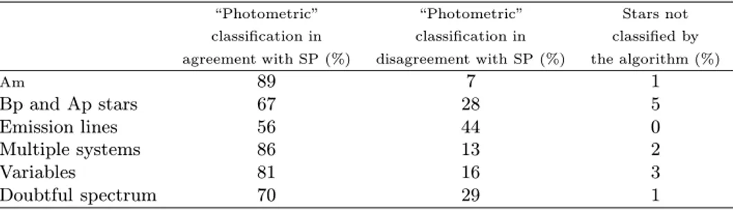
For the intermediate region, Hilditch et al. (1983) pro-posed using m0 as the free parameter to compute E(b− y), but m0 is sensitive to differences in chem-ical composition as it was designed to measure the blanketing. Hilditch et al.’s procedure, slightly mod-ified by Moon (1985), usually overestimates the colour excess. This overestimation of reddening creates empty zones in a colour-colour diagram (see Fig. 4) which are translated onto a histogram of ages as a “deficiency” of stars in certain age ranges. These empty zones are not present in the observed colour-colour diagrams and as such, they are probably an artifact of using m0 as the free parameter. In the present work we dereddened the stars using Grosbøl (1978), which does not produce this effect.
– Dereddening procedure for F stars
In the standard relation for F stars (Crawford 1975) we adopted the values modified by Olsen (1988), cor-responding to β = 2.59 and β = 2.58.
– Dereddening procedure for G3 onwards type stars We adopted the dereddening expressions of Moon (1985) based on Olsen’s (1984) calibration for the re-gion 5 (from G3 onwards). The fact that the calibration by Olsen is only preliminary means that the results for this region should be regarded as being less accurate. The stars with (b− y)0 greater than 0.65 are not dealt with by our algorithm.
0.05 0.10 0.15 0.20 0.25 m1 a) Reddening -0.05 0.00 0.05 0.10 0.15 (b-y)0 0.05 0.10 0.15 0.20 0.25 m0 c) 0.05 0.10 0.15 0.20 0.25 m0 b)
Fig. 4. Intermediate stars in the m1− (b − y) plane. Solid line
is the standard relation Hilditch et al. (1983). a) Observed diagram. b) Intrinsic colours using the procedure proposed by Hilditch et al. (1983) modified by Moon (1985). c) Intrinsic colours using Grosbøl (1978)
3.2. Supergiants
A preliminary calibration of the intrinsic colours of early supergiants was conducted by Zhang (1983) on 157 B-type stars with luminosity classes Ia, Iab, Ib and II. Kilkenny & Whittet (1985) enlarged Zhang’s sample up to about 250 O, B and early A supergiants, and standard relations among (b− y)0, c0and m0were given for each luminosity class.
An iterative process, similar to that of main sequence stars, was introduced in the algorithm to determine in-trinsic from observed colours.
Gray (1991, 1992) discussed the problem of standard calibrations for A, F and G supergiants. He used a sample of supergiants belonging to open clusters, binary systems or near supergiants with published Str¨omgren photome-try to built a new calibration. Arellano Ferro & Parrao (1990) proposed another calibration that partially covers the same spectral types. Here, we chose Gray’s calibra-tions as they cover the full spectral range and, according to the author, were built to be continuous with Kilkenny & Whittet’s (1985) calibration for early supergiants.
Dambis (1991) established an absolute magnitude cal-ibration for stars with 0.12 < [m1]≤ 0.23 (about A4-F3) while Arellano Ferro & Parrao (1990) established a cal-ibration for non-cepheid F0-G8. Both calcal-ibrations were built from supergiants belonging to open clusters and as-sociations. For the range of [m1], where both calibrations were suitable (spectral types F0-F3), we adopted that pro-posed by Arellano Ferro & Parrao. Absolute magnitudes for the early supergiant stars were computed following Balona & Shobbrook (1984).
Table 8 summarizes the calibrations used for the su-pergiants.
Table 7. Calibrations used in each main sequence photometric region
Region Intrinsic colour Mv
1 Crawford (1978) Balona & Shobbrook (1984) 2 Grosbøl (1978) Str¨omgren (1966) 3 Crawford (1979) Crawford (1979) 4 Crawford (1975) Crawford (1975) + Olsen (1988) + Olsen (1988)
5 Olsen (1984) Olsen (1984)
Table 8. Calibrations used in each supergiant photometric region
Region Intrinsic colours Mv
6 Kilkenny & Balona & Whittet (1985) Shobbrook (1984) 7 Gray (1992) Dambis (1991)
+ Arellano Ferro & Parrao (1990) 8 Gray (1991) Arellano Ferro &
4. Analysis of the coherence of the calibrations Since the calibrations used in each region are different, systematic differences in computed colour excesses or dis-tances could be present. The application of the algorithm to stars from open clusters was used as a test of the con-tinuity and agreement among the various calibrations.
The supergiant stars with photometric data belonging to open clusters were used to build the calibrations and so there are no independent data to test them. Thus, the present analysis has been restricted to the main sequence regions.
4.1. The sample of open clusters
The open clusters were selected from the Open Cluster Data Base (Mermilliod 1992). About 60 clusters have more than 20 stars with uvbyHβ. Among the “normal” (in the sense described in Section 2.3) stars in the field of an open cluster we selected the “photometric members”: E(b− y) and distance modulus were computed for each star to-gether with the mean and standard deviation (σ) for each cluster. A star was considered a member of the cluster if its E(b−y) and its distance modulus were both inside the interval mean±2σ. In some cases, two or three iterations were needed until the result was self-consistent. In the case of Mel 20 (α Per), Mel 22 (Pleiades) or Mel 25 (Hyades) we also consulted the published list of members (Prosser 1992; Van Leeuwen et al. 1986; Schwan 1991). This pro-cedure was applied to main sequence stars belonging to photometric regions 1-4 (O-G2 type stars). A star in re-gion 5 was considered a member if being dereddened us-ing the mean E(b− y) of the cluster, its (b − y)0 was in agreement with its spectral type and its distance modu-lus was compatible with that of the cmodu-luster. The reason for this different treatment is the provisional character of Olsen’s (1984) calibration, which might disturb the selec-tion of members for the other regions. After the selecselec-tion of members, the stars in region 5 were dereddened with the algorithm.
The final sample was formed by those clusters satisfy-ing the followsatisfy-ing criteria:
– clusters with 15 members at least, and
– members in at least two different photometric regions. Furthermore, we rejected six clusters (NGC 129, NGC 1342, NGC 1502, NGC 7039, NGC 7062 and IC 4756) that showed very large discrepancies among re-gions or very high standard deviations in the values of E(b− y) or V0− Mv. These were probably due to strong differential reddening or misclassification of members.
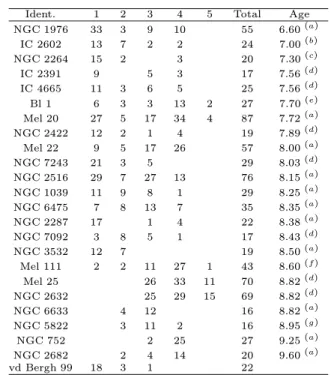
The final sample contained 24 open clusters and 841 stars, listed in Table 9 in ascending order of age. The num-ber of accepted memnum-bers in each main sequence region is also shown in the table.
Table 9. Selected open clusters and number of “photometric” members in each Main Sequence photometric region
Ident. 1 2 3 4 5 Total Age
NGC 1976 33 3 9 10 55 6.60(a) IC 2602 13 7 2 2 24 7.00(b) NGC 2264 15 2 3 20 7.30(c) IC 2391 9 5 3 17 7.56(d) IC 4665 11 3 6 5 25 7.56(d) Bl 1 6 3 3 13 2 27 7.70(e) Mel 20 27 5 17 34 4 87 7.72(a) NGC 2422 12 2 1 4 19 7.89(d) Mel 22 9 5 17 26 57 8.00(a) NGC 7243 21 3 5 29 8.03(d) NGC 2516 29 7 27 13 76 8.15(a) NGC 1039 11 9 8 1 29 8.25(a) NGC 6475 7 8 13 7 35 8.35(a) NGC 2287 17 1 4 22 8.38(a) NGC 7092 3 8 5 1 17 8.43(d) NGC 3532 12 7 19 8.50(a) Mel 111 2 2 11 27 1 43 8.60(f) Mel 25 26 33 11 70 8.82(d) NGC 2632 25 29 15 69 8.82(d) NGC 6633 4 12 16 8.82(a) NGC 5822 3 11 2 16 8.95(g) NGC 752 2 25 27 9.25(a) NGC 2682 2 4 14 20 9.60(a) vd Bergh 99 18 3 1 22 (a)Meynet et al. (1993). (b) Whiteoak (1961). (c) Palous et al. (1977). (d)Mermilliod (1981). (e)Perry et al. (1978). (f) Philip et al. (1977). (g)Hirshfeld (1978). 4.2. Results
In analyzing all the clusters together, for each star we computed the difference between the individual E(b− y) and the mean E(b− y) for the corresponding cluster. The analogous difference was computed in the case of distance modulus. Table 10 shows the mean of these differences for each region and the corresponding standard deviation.
Variance analysis shows coherence at a significance level of 95% between the reddening values computed for the late regions (3 and 4), and statistically significant differences for reddenings computed for regions 1, 2 and 5. The differences decrease by removing NGC 1976 and NGC 2516 clusters from the sample. NGC 1976 is the youngest cluster in the sample with cool stars placed above the ZAMS, which could be pre-main sequence stars. If the E(b− y) for these stars was inaccurate this would artifi-cially introduce a large difference with the reddening of the early region. A large reddening scatter has been reported by several authors (see for example Snowden 1975) for NGC 2516. This scatter can interfer with a right choice of photometric members and might explain the discrepancy among regions.
The use of other calibrations (Hilditch et al. 1983 or Claria 1974) for the intermediate region does not improve the results. The differences are practically the same. The mean differences in region 5 are of the same order as those in other regions, but with a higher standard deviation.
The difficulty in selecting members accurately, the presence of pre-main sequence or unknown binary stars or the differential reddening are several factors that con-tribute to the differences among regions, which, in any case, are lower than the internal errors associated with the calibrations. Taking these facts into account we can conclude that there is good coherence among the calibra-tions used.
For the distance modulus, variance analysis shows co-herence among regions 3, 4 and 5 and between regions 1 and 2, but statistically significant differences between these two groups. The differences among regions are lower than the accuracy of the calibrations, which take in from 0.2m for A-type stars to 0.5m for early B-type stars. It should be borne in mind that an error in E(b−y) causes an error in the determination of V0equal to−4.27 ∆E(b−y) and also in the distance modulus. It is easy to verify from Table 10 that this induced error in V0 is smaller than the discrepancies among regions. So, the differences are mainly due to disagreements in the absolute magnitude calibra-tions. The calibrations for the cooler stars were mainly built from trigonometric parallaxes of nearby stars while for the early and intermediate regions they were based on star members of open clusters. As the former calibra-tions are more accurate, we propose correcting the abso-lute magnitude of the early and intermediate regions, in such a way that the differences quoted in Table 10 disap-pear.
Table 10. Mean values of ∆E(b− y) and ∆(V0− Mv) in the
sense E(b− y)region−E(b − y)cluster, and the same for V0−Mv
Region ∆E(b− y) ∆(V0− Mv) Number
of stars 1 0.005± 0.014 0.04± 0.34 255 2 −0.006 ± 0.015 0.10± 0.29 86 3 −0.001 ± 0.016 −0.05 ± 0.29 211 4 −0.002 ± 0.014 −0.03 ± 0.25 256 5 0.006± 0.039 −0.09 ± 0.30 33
5. Observational and theoretical ZAMS
When the stars are plotted on a colour-colour diagram, in which one colour indicates effective temperature and the other luminosity, the lower envelope of the stars con-stitutes the location of the non-evolved stars (ZAMS). Figure 5 shows various ZAMS defined for the early,
inter-mediate and late photometric regions together with the stars which are members of the clusters in Table 9. For the early and late regions empirical ZAMS were taken from Crawford (1978, 1975, 1979). We refer to Balona & Shobbrook (1984) for the comparison of several ZAMS for the early region. For the intermediate region, Str¨omgren (1966) placed the ZAMS at r = 0. We modified by hand this relation in order to take into account the continuity with the contiguous regions. Table 11 shows the ZAMS adopted for the intermediate region.
Table 11. ZAMS defined for the intermediate region
a0 −0.042 −0.025 0.000 0.025 0.050 0.075 0.084
r 0.006 0.004 0.002 0.001 0.002 0.004 0.006
Effective temperatures and surface gravities of the stars were derived from intrinsic colour indices through Napiwotzki et al.’s (1993) code based on the grids of Moon & Dworetsky (1985) for solar abundance covering the range 6500− 30000 K in Teff and 2.5− 4.5 in log g. The grids were built from the stellar atmosphere models of Kurucz (1979). In line with Jordi et al. (1994), the cor-rection to log g proposed by Napiwotzki et al. for early type stars was not applied. Comparison of the values ob-tained for early type stars with Moon (1985) and Castelli (1991) codes based on the same grids were discussed in Jordi et al. (1994). They found that the systematic differ-ences with determinations of Teff from Geneva photome-try were removed using Napiwotzki et al.’s (1993) code, but that the systematic differences in log g remained. New grids based on revised stellar atmosphere models (Kurucz 1991) are currently being built (Smalley 1995). Preliminary results show the same discrepancy in the sur-face gravity for early type stars.
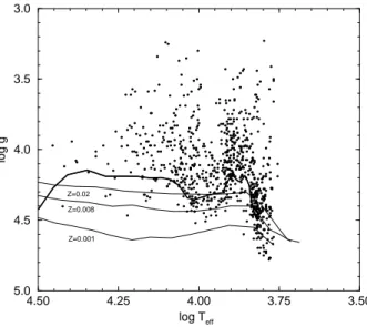
The observational ZAMS translated onto the plane (Teff, log g) using the methods described above are shown in Fig. 6 with the stars belonging to the sample of open clusters. Theoretical ZAMS of stellar evolutionary mod-els reported by Schaller et al. (1992) and Schaerer et al. (1993) at different metallicities are also plotted.
A comparison of different ZAMS was presented by Jordi et al. (1994) for the O-B region and a good agree-ment was found between the theoretical and Crawford’s (1978) observational ZAMS up to 20000 K. The differences in log g for intermediate and late A-type stars (regions 2 and 3) were of 0.1 dex, well within the uncertainty of the log g determinations. As for the early region, good agree-ment was also reported.
At lower temperatures, the observational ZAMS is a good lower envelope of open cluster stars, but it shows a more pronounced slope than the theoretical one, even tak-ing into account different metallicities. The observational ZAMS is placed on the limits of the validity range of the
2.90 2.85 2.80 2.75 2.70 2.65 2.60 2.55 β 0.0 0.2 0.4 0.6 0.8 1.0 1.2 1.4 c0 Crawford 1975, 1979 −0.10 −0.05 0.00 0.05 0.10 0.15 a0 −0.05 0.00 0.05 0.10 0.15 r ZAMS Table 11 Crawford 1978 Crawford 1979 Stromgren 1966 b) −0.2 0.0 0.2 0.4 0.6 0.8 1.0 1.2 c0 3.00 2.90 2.80 2.70 2.60 2.50 β Crawford 1978 a) c)
Fig. 5. Observational ZAMS for a) early, b) intermediate and c) late regions. Dots are the members of open clusters in Table 9
grids. The determination of Teff and log g may be uncer-tain, but whether this is the reason for the discrepancy, or whether it is due to a real difference between obser-vational and theoretical ZAMS is a matter that requires further research.
The conclusions drawn from this comparison are sim-ilar if the theoretical models by Claret & Gim´enez (1992) are considered instead of those of Schaller et al. For a comparison among recent stellar evolutionary models see Asiain et al. (1997). 4.50 4.25 4.00 3.75 3.50 log Teff 5.0 4.5 4.0 3.5 3.0 log g Z=0.001 Z=0.008 Z=0.02
Fig. 6. Observational and theoretical ZAMS plotted with the open cluster star members of Table 9. Thin lines represent the theoretical ZAMS proposed by Schaller et al. (1992) and Schaerer et al. (1993) at different metallicities. The thick line represents observational ZAMS (see text)
6. Conclusions
We have described an algorithm to classify stars into pho-tometric regions based on Str¨omgren indices. The algo-rithm enlarges that described in Figueras et al. (1991) and covers as much of the HR diagram as possible, includ-ing the supergiant stars. The application of the algorithm to a large sample of stars shows its validity: about 90% of “normal” single stars are photometrically classified in agreement with their spectral type and luminosity class; for peculiar, emission line or binary stars this percentage is slightly lower.
The calibrations used to calculate intrinsic colours and absolute magnitudes in each photometric region have been presented and discussed. To study the coherence of the calibrations we applied them to stars from open clusters. Some differences were found between the mean values for each photometric region. In the case of the absolute mag-nitudes there was a discrepancy between the results ob-tained for the early and intermediate regions and those for the late region. We can conclude that there is a good agree-ment among currently available calibrations for E(b− y), but not for those of Mv. This would suggest the need for a correction in the Mvcalibration for early and intermediate regions.
The agreement between observational and theoretical ZAMS has also been studied. It was found to be satisfac-tory within the uncertainty of the determinations in Teff and log g, for B and A type stars. However, for F-type stars there is an evident discrepancy between observational and theoretical ZAMS.
The availability of new data, especially accurate trigonometric parallaxes from Hipparcos satellite, and the revision of stellar atmosphere models, should help to im-prove the calibrations and thus avoid existing discrepan-cies.
Acknowledgements. We would like to thank J.C. Mermilliod for kindly suppling us with his Open Cluster Data Base. This work was supported by the CICYT under contract ESP95-0180. E.M. acknowledges financial support from the Ministerio de Educaci´on y Ciencia.
References
Arellano Ferro A., Parrao L., 1990, A&A 239, 205 Asiain R., Torra J., Figueras F., 1997, A&A (in press) Balona L.A., Shobbrook R.R., 1984, MNRAS 211, 375 Castelli F., 1991, A&A 251, 106
Claret A., Gim´enez, A., 1992, A&AS 96, 255
Claria J.J., 1974, Elementos de Fotometr´ıa Estelar, Instituto Venezolano de Astronom´ıa
Comer´on F., Torra J., Jordi C., G´omez A.E., 1993, A&AS 101, 37
Crawford D.L., 1975, AJ 80, 955 Crawford D.L., 1978, AJ 83, 48 Crawford D.L., 1979, AJ 84, 1858
Crawford D.L., Mandwewala N., 1976, PASP 88, 917 Dambis A.M., 1991, Soviet Astron. Lett. 17, 307 Figueras F., Torra J., Jordi C., 1991, A&AS 87, 319 Gray R.O., 1991, A&A 252, 317
Gray R.O., 1992, A&A 265, 704 Grosbøl P.J., 1978, A&AS 32, 409 Guthrie B.N., 1987, MNRAS 226, 361
Hauck B., Mermilliod J.C., 1990, A&AS 86, 107
Hilditch R.W., Hill G., Barnes J.V., 1983, MNRAS 204, 241 Hirshfeld A., McClure R.D., Twarog B.A., 1978, IAU Symp.
80, 163
Jakobsen A.M., 1985, PhD Thesis, University of Aarhus, Denmark
Jordi C., Trullols E., Rossell´o G., Lahulla F., 1992, A&AS 94, 519
Jordi C., Masana E., Figueras F., Torra J., Asiain R., 1994, Space Sci. Rev. 66, 203
Jordi, C., Figueras F., Torra J., Asiain R., 1996, A&AS 115, 401
Kilkenny D., Whittet D.C.B., 1985, MNRAS 216, 127 Kurucz R.L., 1979, ApJS 40, 1
Kurucz R.L., 1991, in Precision Photometry: Astrophysics of the Galaxy, Philip A.G.D., Upgren A.R., Janes K.A.L. (eds.). Davis Press, Schenectady, N.Y., p. 27
Mermilliod J.C., 1981, A&A 97, 235
Mermilliod J.C., 1992, Bull. Inform. CDS No. 40, 115 (June 1995 version)
Meynet G., Mermilliod J.-C., Maeder A., 1993, A&AS 98, 477 Moon T.T., 1985, Communication from the University of
London Observatory, No. 78
Moon T.T., Dworetsky M.M., 1985, MNRAS 217, 305 Napiwotzki R., Sch¨onberner D., Wenske V., 1993, A&A 268,
653
Oblak E., Consid`ere S., Chareton M., 1976, A&AS 24, 69 Olsen E.H., 1984, A&AS 57, 443
Olsen E.H., 1988, A&A 189, 173
Palous J., Ruprecht J., Dluzhnevskaya O.B., Piskunov T., 1977, A&A 61, 27
Perry C.L., Walter D.K., Crawford D.L., 1978, PASP 90, 81 Philip A.G.D., Miller T.M., Relyea L.J., 1976, Dudley Obs.
Reports, No. 12
Philip A.G.D., Demarque P., Sweigart A.V., Ciardullo R.B., 1977, PASP 89, 554
Prosser C.F., 1992, AJ 103, 488
Schaerer D., Charbonnel C., Meynet G., Maeder A., Schaller G., 1993, A&AS 102, 339
Schaller G., Schaerer D., Meynet G., Maeder A., 1992, A&AS 96, 269
Schwan H., 1991, A&A 243, 386
Smalley, B., 1995 (private communication) Snowden M.S., 1975, PASP 87, 721 Str¨omgren B., 1966, ARA&A 4, 433 Turon C., et al., 1992, ESA SP-1136
van Leeuwen P., Alphenaar P., Brand J., 1986, A&AS 65, 309 Whiteoak J.B., 1961, MNRAS 123, 245
![Fig. 1. [u − b] − β diagram for stars with spectral types O-A3. The solid line represents the criterion given by Philip et al](https://thumb-eu.123doks.com/thumbv2/123dokorg/4444127.30289/2.918.464.817.350.637/diagram-stars-spectral-types-represents-criterion-given-philip.webp)