Analysis of a gradual Solar Energetic Particle event
Author: David Rodríguez Ramos
Facultat de Física, Universitat de Barcelona, Diagonal 645, 08028 Barcelona, Spain*.
1. Abstract
This present paper is concerned about the analysis of a solar energetic particle (SEP) event. Those particles are associated to solar activity. A particular event is studied, and by applying the theoretical laws through some calculations, its solar origin is found. Hence the original solar activity, which was the cause of the SEP event, is confirmed. If a solid theory between solar activity and SEP is established, the forecasting of the space weather would be possible, and this way allowing the prevention of damage on satellites, spacecrafts, astronauts during spacewalks; or even in Earth systems such as commercial aeroplanes or antennas.
2. Introduction
2.I Solar Energetic Particle event
Everything in the solar system is under the influence of space weather, which is regulated by the Sun and its phenomena. Solar activity ejects particles, known as solar wind, out to the interplanetary medium and the components of solar wind are mostly SEP particles: mainly protons, electrons, He+ ions and HZE ions.
SEP are a highly important scientific issue to study. On one hand they constitute the main element of solar wind, which is the defining component of solar radiation storms who have effect on any element in the solar system. On the other hand, the study of SEP states the opportunity to analyse their acceleration mechanisms, transport processes and sources; therefore providing the testing of the energetic particles propagation theories with in-situ measurements.
Depending on their features SEP events are divided in gradual or impulsive events. However, these two categories are not perfectly divided and most of the events collide on a third category called mixed events. Their main difference rely on their starting processes. While impulsive ones have a more energetic origin, therefore are more ionized and have a superior enhancement of isotopes –and are electron rich; the gradual ones, as they are less energetic, have the same composition as the solar corona and are proton rich.
This project is the study of a gradual event, so it will not go further in details about impulsive events.
SEP events are associated either to solar flares or coronal mass ejections (CMEs), both of them are activities on the Sun. Even though they are different processes, a CME can happen with a solar flare.
SEP events related to solar flares represent the outflow of particles during magnetic reconnection in active regions. SEP related to CME are particles that are produced by an acceleration at a collisionless shock wave driven by the CME. Those shock-accelerated particles propagate along interplanetary magnetic field (IMF) lines. The magnetic connection to the shock that accelerates the particles is a crucial factor when determining the intensity profile of SEP events: when this magnetic connection between the observer and the field lines where these particles propagate is established, a particle’s flux enhancement is observed at the detectors in space.
Additionally, interplanetary scattering is thought to be of minor importance in determining the observed profiles. In this project, the case of study is the event that was undertaken on the 4th of April 2000 in which, data analysis has been applied to determine the onset time and the flying time of the particles. Hence correlate the SEP event with the solar fulgurations that originate it.
2. II Instrumentation and data description
To acquire the data that it has been used in this project two spacecraft were used:
GOES
Geostationary Operational Environmental Satellite was consulted for data about particle flux. GOES detectors measure proton, alpha particle and electron fluxes by pulse-height discrimination. Although protons that are in the database have been partially corrected for contaminated particles, protons from other sources may appear, especially for low energies.
ACE
The Advanced Composition Explorer is a NASA satellite whose objective is to study and determine the composition of several types of matter such us solar wind or interstellar medium. It is placed at Lagrangian point 1, between the Sun and the Earth.
ACE/MAG
The Magnetic Field Experiment of ACE (MAG) consists of two twin magnetometers placed 4.19 meters away from the center of the spacecraft. They are at opposite sides along de Y axis of ACE. Both sensors are controlled by a common CPU. ACE/MAG data has been used to provide data of the magnetic field of the solar wind in RTN system. This data has a period time of observation of 16 seconds.
ACE/SWEPAM
The solar Wind Electron, Proton, and Alpha Monitor (SWEPAM) has been used for measuring solar wind conditions (speed, temperature and density of the protons). It provides a real-time solar wind observation which is continuously being emitted to the ground system. It measures in several time ranges. In this project it has been used the range which provides an observation each 64 seconds.
3. Data Analysis Methods 3. I Solar release time determination
The release time is defined as the time at which particles were thrust out of the sun. It is assumed that there is no dependence on the energy of the particles, meaning that the release time will have the same value for all of the particles. In order to calculate it is necessary to know how much time particles spent travelling from Sun to Earth and when did particles reach the detector. It is important to point out that although it is not a prompt event, it has a duration on time, meaning that there is not an exact release time, it will be considered as a sharp peak emission which is placed at the release time.
Particles will follow the magnetic field line that connects the sun region with the satellites. So the path that solar particles will describe is a Parker spiral. The length of this spiral is a function that depends on the speed of solar wind and the distance at which the spacecraft is located. The velocity dispersion equation at 1 AU can be written as it follows:
tonset = trelease +8,33
𝐿(𝑧) 𝛽(𝐸)
tonset - trelease = tfly = 8,33
𝐿(𝑧) 𝛽(𝐸)
Where tonset [minutes] is defined as the time at which the
data of the detectors shows a rise in the incoming particles’ flux. Meaning that the early particles of the event reached out the detector. L(z) [AU] is the length that particles travelled since they left the Sun and reached the Earth distance. β is the inverse speed of the particles defined as 𝛽 =𝑣
𝑐
To calculate the length of the path that protons are travelling is used the nominal length of Parker Spiral. Protons will lead from solar corona and will end their trajectory at the detectors. Hence the distance will be: L(z) = Z(satellite) – Z(Rsun) 𝑧 = 𝑎 2 [ ln ( 𝑟 𝑎+ √1 + ( 𝑟 𝑎) 2 ) + 𝑟 𝑎 √1 + ( 𝑟 𝑎) 2 ] (1) (2)
Where a is defined as 𝑣𝑠𝑤
𝛺𝑠𝑢𝑛 and 𝛺𝑠𝑢𝑛 is related to the
equatorial period of solar rotation in this way: 2π𝛺𝑠𝑢𝑛 = 24,47 days. Hence these two variables are
necessary to calculate the release time: solar wind speed and onset time.
3. III-A Analysis of the 2nd of April 2000 event
FIG 1. Data plot of particles flux by energy channel, solar wind velocity, density and temperature, magnetic field between doys * 94 to 99. *Day Of the Universe
After processing detectors data and plotting it several features can be seen. It is observed that flux intensities rise several order of magnitude before doy 95,8.. So the event under study started the afternoon of 95 doy. Besides its shock wave reached Earth distance the afternoon of 97 doy affecting on almost all parameters.
Lowest energy channel (0,8 – 4,0 MeV) shows several fluctuations due to interferences with particles in the Earth’s atmosphere. The lower the energy is, the more abundant the particles are. Moreover at 96,8 doy all channels are saturated, there is a resonance effect for all detectors.
As there is no significant jump for high energies, there have only been used energy channels below 40 MeV. For low energy channels, tonset is determined by visual
evidence on the particle intensity profile.
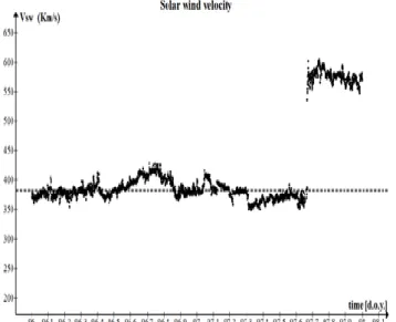
3. III-B solar wind velocity determination
Solar wind is considered to be constant before the shock, the average value of the solar wind will be used to do the calculations.
FIG 2. Showsp+ velocity profile between doy 96 and 98.1 There is a small fluctuation out of the line between 96.6 and 96.8 doys. Although there is no theoretical reason not to consider these values, calculations will be repeated for the scenario in which this fluctuation eliminated (2), as they presumably have a different source.
Solar wind average: Vsw = 382,7 km/s
Solar wind average (2): 𝑉
𝑠𝑤 (2)
Hence Length of Parker Spiral:
1,8· 1011 ± 0,4· 1011 m = 1,19 AU ± 0,25AU
TABLE 1 Different time of reference was used where t’ = 0 at
noon of doy 95.
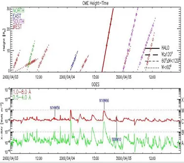
3. IV Solar activity observation
TABLE 2 X-Ray flare characteristics in the Virtual Solar Observator
FIG. 3 Analysis of the CME and Solar Flare (N16 W66) related to the event
4. Conclusions.
Energy channel (MeV)
Time of release Time of release (2) 0,8 – 4,0 15:39 ± 8 min 14:54 ± 8 min
4,0 – 9,0 16:08 ± 6 min 15:43 ± 6 min
9,0 – 15,0 16:14 ± 6 min 15:55 ± 6 min
15,0 – 40,0 16:21 ± 6 min 16:07 ± 6 min
TABLE 3 Comparison between the observational time of release and the calculated time of release
In spite of the fact that solar flare observations are off the calculated intervals, this results prove that this SEP event is related to the solar activity seen on the observations (N16 W 66) at 15:41.
Since the theoretical scenario is not fully understood, most of the assumptions are rough.
The final uncertainty in time is about 8 minutes at most. However, the whole solar flare lasts 20 minutes. Whereas it is no possible to know when particles that reach the detector were released, it has been assumed that they were on the peak of activity; and this is not necessarily true.
Particles were supposed to follow solar magnetic field lines. Nonetheless, how the shockwave propagation and the CME affects the magnetic structure is not fully understood. Consequently, this line might differ to the Parker Spiral’s shape that was assumed and path length calculations might not be realistic.
Another assumption was that particles velocity was constant during fly time. It happens not to be true, particles are slowing down as they get further of the Sun. Moreover when the data analysis was repeated, neglecting those points that were off of the average value, results were more accurate so it seemed that this rise of the flux came from a different source. Still, there is not theoretical reason to eliminate this fluctuation.
Background noise for low energy channels, especially in the first trial, has appeared to be of a greater importance introducing a big deviation in the final result for this energy framework. Energy Channel (Mev) Mean Energy (Mev) β (𝑣 𝑐⁄ ) tfly (minutes) t’ (95,5) (minutes) 0,8 – 4,0 1,8 0,0617 158 ± 3 380 ± 5 4,0 – 9,0 6,0 0,1126 86 ± 3 337 ± 3 9,0 – 15,0 11,6 0,1559 62 ± 3 318 ± 3 15,0 – 40,0 24,5 0,2241 43 ± 3 307 ± 3 40,0 – 80,0 56,6 0,3324 29 ± 3 --- 80,0 – 165,0 114,9 0,4542 21 ± 1.5 --- 165,0 – 500,0 287,2 0,6433 15± 1 --- Flare start Flare end Flare max Position Flare class Intensity 15:21:00 16:05:00 15:41:00 N16W66 C 9.7
Lastly, instead of using visual perception to find tonset
there are algorithms that through iterative methods find this time certainly.
In order to increase accuracy more energy channels should be use. Ideally, narrow channels between the energies regions of interest. With several energy channels it is possible to plot a diagram tonset vs. 1/β and use this
plot to fin the release time minimizing deviations. Nevertheless there is a technical barrier as the number of detectors is limited because they are out in space making it an experiment hard to manipulate.
To conclude, as this is a hard field to study since the only way to have a detector is sending a spacecraft out to the space; this experiment shows rough assumptions. However final results are plausible and allow to work on them, meaning an initial step forward on the knowledge of the space weather; and in second level about particle transport physics. By acquiring this knowledge, space weather forecasting may be possible in a near future, allowing agencies to avoid damages during solar storms. Furthermore, this Sun-Earth interaction knowledge might be extrapolated to other star-planet system.
5. Appendix
These uncertainties were used during the present project.
(3) (4) (5) AKNOWLEDGEMENTS
I would like to acknowledge Professor Angels Aran for guiding me through the data acquisition process; my partner for its inestimable help and patientience and; finally, my tutor, Professor Blai Sanahuja for his wisdom, advices, support and field experience throughout the whole process. Thank you.
_______________________________________________________________ 6. Bibliography
Malandraki, et al., Scientific Analysis within SEPServer – New Perspectives in Solar Energetic Particle Research: The Case Study of the 13 July 2005 Event (Springer science+Business Media Dordrecht, 2012)
Vainio, et al. The first SEPServer event catalogue ~68-MeV solar proton events observed at 1 AU in 1996–2010 (EDP Sciences, 2013)
Emilio et al. Measuring the Solar Radius from Space during the 2003 and 2006 Mercury Transit (Standford University, 2012)
Donald V Reames Particle acceleration at the sun and in the heliosphere (Space Science Reviews, 1999)
Committee on Solar and Space Physics and Committee on Solar and Terrestrial Research, National Research Council. Radiations and the international space station (2000)
GOES http://satdat.ngdc.noaa.gov/sem/goes ACE: http://www.srl.caltech.edu/ACE/ASC/level2/index.html http://cdaw.gsfc.nasa.gov/CME_list/UNIVERSAL/2000_04/univ2000_04.html
http://www.ssg.sr.unh.edu/mag/ace/ACElists/obs_list.html#shocks http://vso.nso.edu/cgi/catalogui?