Efficient Semantic Matching

(1)

UNIVERSITY

OF TRENTO

DEPARTMENT OF INFORMATION AND COMMUNICATION TECHNOLOGY

38050 Povo – Trento (Italy), Via Sommarive 14

http://www.dit.unitn.it

EFFICIENT SEMANTIC MATCHING

Fausto Giunchiglia, Mikalai Yatskevich

and Enrico Giunchiglia

December 2004

Technical Report # DIT-04-112

(2)

(3)

Efficient Semantic Matching

Fausto Giunchiglia1, Mikalai Yatskevich1, Enrico Giunchiglia2

1_{Dept. of Information and Communication Technology}

University of Trento, 38050 Povo, Trento, Italy {fausto, yatskevi}@dit.unitn.it

2

DIST – Universita di Genova Viale Causa 13, 16165, Genova, Italy

enrico@dist.unige.it

Abstract. We think of Match as an operator which takes two graph-like

structures and produces a mapping between semantically related nodes. We concentrate on classifications with tree structures. In semantic matching, correspondences are discovered by translating the natural language labels of nodes into propositional formulas, and by codifying matching into a propositional unsatisfiability problem. We distinguish between problems with conjunctive formulas and problems with disjunctive formulas, and present various optimizations. For instance, we propose a linear time algorithm which solves the first class of problems. According to the tests we have done so far, the optimizations substantially improve the time performance of the system.

1. Introduction

We think of matching as the task of finding semantic correspondences between elements of two graph-like structures (e.g., conceptual hierarchies, classifications, database schemas or ontologies). Matching has been successfully applied in many well-known application domains, such as schema/ontology integration, data warehouses, and XML message mapping. In this paper we concentrate on classifications with tree structures.

Semantic matching, as introduced in [1, 5], is based on the key intuition that labels at nodes, which are written in natural language, are translated into propositional formulas which codify the intended meaning of the labels themselves. This allows us to codify the matching problem into a propositional unsatisfiability problem, which can then be efficiently implemented using state of the art propositional satisfiability (SAT) solvers [8, 9]. We call concept of a label the propositional formula which stands for the set of documents that one would classify under a label it encodes. We call concept at a node the propositional formula which represents the set of documents which one would classify under a node, given that it has a certain label and that it is in a certain position in a tree [5]. As from [5], all previous approaches, though implicitly or explicitly exploiting the semantic information codified in graphs, differ substantially from our approach in that they compute a syntactic “similarity” coefficients between labels in the [0,1] range (see for instance [3, 10] ).

(4)

The system we have developed, called S-Match [6], takes two classifications and computes the strongest semantic relation holding between any pair of nodes. The matching problem is articulated into two macro steps, namely element and structure level matching. Element level matchers consider only the information on the atomic level [7] (the labels of nodes), while structure level matchers consider also the structure of the trees. Our goal in this paper is to describe the structure level matching algorithm, as it has been implemented within S-Match, and present a set of optimizations. In particular, we distinguish between two main classes of problems. In the first class all the concepts at nodes are atomic or conjunctive formulas. In the second class the concepts at nodes may also contain disjunctive formulas. In the case of conjunctive concepts at nodes we present a modification of the original algorithm which solves the node matching problem in linear time. With disjunctive concepts we present various techniques, which, among the other things, allow us to avoid the exponential space explosion which arises when converting disjunctive formulas into Conjunctive Normal Form (CNF). This modification is required since all state of the art SAT deciders take CNF formulas in input.

We have evaluated the time performance of the optimized algorithm against its basic version and several state of the art matching systems. The optimizations seem to improve substantially the time performance of S-Match. In all cases S-Match performs better or much better than the unoptimized version and always competes well with the other matching systems. In particular, it outperforms them on trees with hundreds or thousands of nodes.

The rest of the paper is organized as follows. Section 2 provides an overview of the

S-Match tree matching algorithm. Section 3 discusses the basic node matching

algorithm. The next two sections are dedicated to the two classes of node matching problems we have identified. Node matching problems with conjunctive concepts at nodes (and their optimizations) are discussed in Section 4, while the node matching problems with disjunctive concepts at nodes (and their optimizations) are described in Section 5. We discuss the evaluation results in Section 6. Section 7 concludes the paper.

2. The tree matching algorithm

As from [6], the S-Match algorithm is organized according the following four macro steps:

− Step 1: for all labels in the two trees, compute concepts of labels;

− Step 2: for all nodes in the two trees, compute concepts at nodes;

− Step 3: for all pairs of labels in the two trees, compute the semantic relations between concepts of labels;

− Step 4: for all pairs of nodes in the two trees, compute the semantic relations between concepts at nodes.

The first two steps represent the pre-processing phase, while the third and the fourth steps correspond to the element-level and structure-level matching respectively. The semantic relations we consider are: equivalence (=); more general

(5)

(⊇); less general (⊆); disjointness (⊥); overlapping (∩). When none of the relations holds, the special Idk (I don’t know or (?)) relation is returned.

The version of the algorithm defined in this paper assumes that:

− There are no negated atomic concepts of labels (one example of negated concept of label is Cexcept apple=¬Capple)

− The information we use, namely the labels of nodes and the knowledge residing in WordNet (see below) is all globally consistent. Under this assumption the only reason why we get an unsatisfiable formula is because we have found a match between two nodes

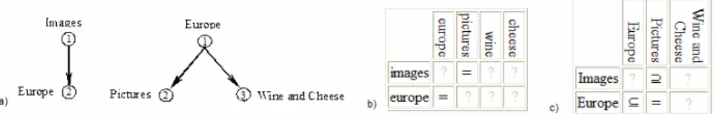
In order to understand how the algorithm works, consider for instance the two trees depicted in Figure 1a.

Fig. 1. (a): Two trees. (b): The matrix of relations between concepts of labels. (c): The matrix

of relations between the concepts at nodes (matching result).

During Step 1 we first tokenize labels. For instance “Wine and Cheese” becomes <Wine, and, Cheese>. Then we lemmatize tokens. Thus for instance “Images” becomes “image”. Then, an Oracle (at the moment we use WordNet 2.0) is queried in order to obtain the senses of the lemmatized tokens. Afterwards, these senses are attached to atomic concepts. Finally, complex concepts are built suitably composing atomic concepts. Thus, the concept of the label Wine and Cheese is computed as CWine and Cheese = <wine, {sensesWN#4}>∨<cheese, {sensesWN#4}>, where <cheese, {sensesWN#4}> is taken to be the union of the four WordNet senses, and similarly for wine. Notice that natural language and is converted into logical disjunction rather than

conjunction.

Step 2 takes into account the structural schema properties. The logical formula for

a concept at a node is constructed most often as the conjunction of the concept of a label formulas in the concept path to the root [5]. For example, the concept C2 for the

node Pictures in Figure 1a is computed as C2=CEurope ∧ CPictures.

Element level semantic matchers are applied during Step 3. They determine the semantic relations holding between pairs of atomic concepts of labels. For example, from WordNet we can derive that image and picture are synonyms, and therefore, CImages = CPictures. Notice that Image and Picture have 8 and 11 senses in WordNet,

respectively. In order to determine the senses which are relevant in the current context, sense filtering techniques are applied (see [11] for more details). The relations between the atomic concepts of labels for the trees depicted in Figure 1a are reported in Figure 1b.

Element level semantic matchers provide the input to the structure level matcher, which is applied in Step 4. This matcher produces the set of semantic relations between concepts at nodes (see Figure 1c for example). On this step the tree matching problem is reformulated into the set of node matching problems, one for each pair of

(6)

nodes. Further, each node matching problem is reduced to a propositional validity problem.

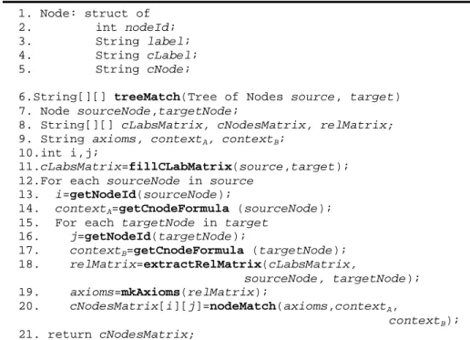
The pseudo code of the Steps 3 and 4 of the semantic matching algorithm is reported in Figure 2. treeMatch takes 2 trees of Nodes (source, target) and returns the matrix of semantic relations between concepts at nodes in both trees (cNodesMatrix). First, fillCLabMatrix exploit element level semantic matchers library in order to fill the matrix of relations between concepts of labels in both trees (cLabsMatrix) (line 11). This action corresponds to the third step of the tree matching algorithm. Afterwards, two loops over all nodes of source and target trees are executed (lines 12-20 and 15-20). Within these loops, the propositional formulas corresponding to the concepts at nodes (contextA, contextB) are computed by getCnodeFormula (lines 14, 17).

1. Node: struct of 2. int nodeId; 3. String label; 4. String cLabel; 5. String cNode;

6.String[][] treeMatch(Tree of Nodes source, target) 7. Node sourceNode,targetNode;

8. String[][] cLabsMatrix, cNodesMatrix, relMatrix; 9. String axioms, contextA, contextB;

10.int i,j;

11.cLabsMatrix=fillCLabMatrix(source,target); 12.For each sourceNode in source

13. i=getNodeId(sourceNode);

14. contextA=getCnodeFormula (sourceNode); 15. For each targetNode in target

16. j=getNodeId(targetNode); 17. contextB=getCnodeFormula (targetNode); 18. relMatrix=extractRelMatrix(cLabsMatrix, sourceNode, targetNode); 19. axioms=mkAxioms(relMatrix); 20. cNodesMatrix[i][j]=nodeMatch(axioms,contextA, contextB); 21. return cNodesMatrix;

Fig. 2. The pseudo code of the tree matching algorithm.

relMatrix is calculated in the inner loop by extractRelMatrix (line 18). It contains the part of the cLabsMatrix relevant to the particular node matching problem. axioms (line 19) contains the conjunction of the propositional formulas in

relMatrix. For example, the semantic relations in Figure 1b, which are considered

when we match Europe and Pictures are EuropeA= EuropeB, ImagesA= PicturesB. In

this case axioms is (EuropeA ↔ EuropeB)∧ (ImagesA ↔ PicturesB). Notice that,

subscripts designate the context (either A or B) to which a propositional variable (or concept) belongs. The detailed description of nodeMatch is provided in the next section.

(7)

3. The node matching algorithm

nodeMatch input formulas are combined to obtain the following formula:

(axioms) → rel(contextA , contextB ), (1) where axioms, contextA, contextB are as defined in treeMatch (Figure 2), while rel(contextA , contextB ) is the formula corresponding to the semantic relation being

checked, (namely equivalence, less or more generality, or disjointness). As from [5], two nodes match if and only if Eq. 1 is valid, namely if it is true for all possible truth assignments to its propositional variables. Given that most of the available propositional solvers are satisfiability checkers, the negation of the matching formula is checked for unsatisfiability. This yields the following formula

axioms ∧¬ rel(contextA , contextB ) (2)

Table 1 reports the resulting matching formulas as a function of the semantic relation being tested. Notice that the check for equality is omitted. In fact A=B holds iff A⊆B and A⊇B hold.

Table 1. The relationship between semantic relations and propositional formulas.

rel(a,b) Translation of rel(a, b)

in propositional logic CNF translation of Eq. 2

a=b a↔b N/A

a⊆b a→b axioms∧contextA∧ ¬contextB

a⊇b b→a axioms∧contextB∧ ¬contextA

a⊥b ¬(a∧b) axioms∧contextA∧ contextB

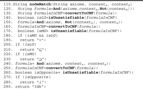
Consider the pseudo code of the node matching algorithm, as described in Figure 3.

110.String nodeMatch(String axioms, contextA, contextB) 120. String formula=And(axioms,contextA,Not(contextB));

130. String formulaInCNF=convertToCNF(formula); 140. boolean isLG=isUnsatisfiable(formulaInCNF) 150. formula=And(axioms, Not(contextA), contextB); 160. formulaInCNF=convertToCNF(formula);

170. boolean isMG= isUnsatisfiable(formulaInCNF); 180. if (isMG && isLG)

190. return “=”; 200. if (isLG) 210. return “⊆”; 220. if (isMG) 230 return “⊇”;

240. formula= And(axioms, contextA, contextB); 250. formulaInCNF=convertToCNF(formula);

260. boolean isOpposite= isUnsatisfiable(formulaInCNF); 270. if (isOpposite)

280. return “⊥”; 290. return “Idk”;

(8)

nodeMatch constructs the formulas needed for testing less generality (line 120) and more generality (line 150), it converts them to CNF (lines 130, 160) and checks for unsatisfiability (lines 140, 170). If both relations hold, then the equivalence relation is returned (line 190). Afterwards, the same procedure is repeated for disjointness test. If all the tests fail “Idk” is returned (line 290).

Prior to the discussion of optimizations to our basic solution, let us classify the concepts of labels and concepts at nodes. We distinguish between four categories of

concepts of labels:

− Atomic: the concept of a label is an atomic proposition. For example, the concept of the label Europe is CEurope = <Europe, {sensesWN#1}>, where sensesWN#1 stands

for a WordNet sense.

− Conjunctive: the concept of a label is a conjunction. For example, the concept of the label transmission gearbox is Ctransmission gearbox = Ctransmission∧Cgearbox.

− Disjunctive: the concept of a label is a disjunction. For example, the concept of the label jet and trains and cars is Cjet and trains and cars=Cjet∨Ctrain∨Ccar.

− Full proposition at logic: the concept of a label contains both conjunctions and disjunctions. For example the concept of the label computers and electrical

equipment is Ccomputers and electrical equipment=Ccomputer∨ (Celectrical∧C equipment)

This classification allows us to further distinguish between two classes of concepts

at nodes, which are at the basis of our optimizations:

− Conjunctive concepts at nodes: the concept at a node is a conjunction.

− Disjunctive concepts at nodes: the concept at a node contains both conjunctions and disjunctions in any order.

4. Conjunctive concepts at nodes

4.1 Node matching problems

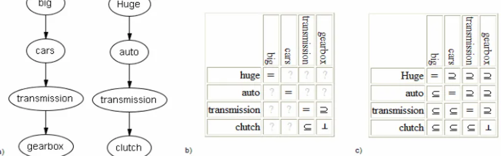
Consider the two trees depicted in Figure 4a. Notice that they have only atomic concepts of labels. Let us consider the matching of gearbox and clutch.

Fig. 4. (a): Two trees. (b): The matrix of relations between concepts of labels. (c): The matrix

(9)

The relevant semantic relations between concepts of labels are depicted in Figure 4b. As from Table 1, axioms is:

(bigA↔hugeB)∧(carA↔autoB) ∧ (transmissionA↔ transmissionB )∧ (gearboxA→transmissionB) ∧(clutchB→transmissionA)∧ ¬(clutchB∧gearboxA)

(3) which, translated in CNF, becomes:

(¬bigA∨hugeB)∧(bigA∨¬hugeB)∧(¬carA∨autoB)∧(carA∨¬autoB) ∧ (¬transmissionA∨ transmissionB ) ∧ (transmissionA∨¬ transmissionB ) ∧ (¬gearboxA∨transmissionB)∧(¬clutchB∨transmissionA)∧(¬clutchB∨¬gearboxA)

(4) As from Step 2 in Section 2, contextA and contextB are constructed by taking the

conjunction of the concepts of labels in the path to root. Therefore, contextA and contextB are:

bigA∧carA∧transmissionA∧gearboxA (5)

hugeB∧autoB∧transmissionB∧clutchB (6) while their negations are:

¬bigA∨¬carA∨¬transmissionA∨¬gearboxA (7)

¬hugeB∨¬autoB∨¬transmissionB∨¬clutchB (8)

Let us consider the formula to be checked for unsatisfiability, as from Table 1. The first observation is that axioms remains the same for all the tests, and it contains only clauses with two variables, where a clause is a finite disjunction of literals. In the worst case it contains 2*nA*nB clauses, where nA and nB are the number of atomic

concepts of labels in the paths to the root (in our example nA and nB are equal to 4).

The second observation is that the formulas for less and more generality are very similar and differ only in the context formula which is negated. Thus, for instance, in the less generality test contextB is negated. This means that Eq. 1 contains one clause

with nB variables (Eq. 8) in addition to nA clauses with one variable derived from contextA (Eq. 5). Finally, again from Table 1, in the case of disjointness test contextA

and contextB are not negated. Therefore, Eq. 1 contains nA+nB clauses with one

variable (Eq. 5 and Eq. 6).

So far we have concentrated on atomic concepts of labels. The propositional formulas remain the same if we move to conjunctive concepts at labels. Consider the trees depicted in Figure 5a. Let us consider the matching between transmission

gearbox and transmission clutch.

Fig. 5. (a): Two trees. (b): The matrix of relations between concepts of labels in the trees. (c):

(10)

Compare the matrices on the Figure 5b and Figure 4b. They are the same. The matrix of the relations between concepts of labels unambiguously determines axioms (see Eq. 3 and 4). Furthermore, as from Step 2 in Section 2, the propositional formulas for contextA and contextB are the same for atomic and for conjunctive

concepts of labels as long as they “globally” contain the same formulas. In fact, concepts at nodes are constructed by taking the conjunction of concepts at labels. Splitting a concept of a label with two conjuncts into two atomic concepts has no effect on the resulting matching formula.

4.2 Optimizations

Let us consider first more and less generality and then disjointness.

4.2.1 Less and more generality tests

As from Section 4.1, formula (Eq. 1) in this case is as follows:

(9)

where n is the number of variables in contextA, m is the number of variables in contextB. Ai’s belong to contextA, and Bj’s belong to contextB. s, k, p are in the [0..n]

range, while t, l, r are in the [0..m] range. Axioms can be empty. Eq. 9 is composed of clauses with 1 or 2 variables plus one clause with possibly more variables (the clause corresponding to the negated context). The key observation is that the formula in Eq. 9 is Horn: each clause contains at most one positive literal. Therefore, the satis? ability problem can be decided in linear time by the unit resolution rule [2]. Notice, that DPLL-based SAT solvers require quadratic time in this case [15].

In order to understand how the linear time algorithm works, let us prove the unsatisfiability of Eq. 9 in the case of gearbox and clutch. In this case, Eq. 9 becomes

((¬bigA∨hugeB)∧(bigA∨¬hugeB)∧(¬carA∨autoB)∧(carA∨¬autoB)∧ (¬transmissionB∨ transmissionA ) ∧ (transmissionB∨¬ transmissionA ) ∧

(¬gearboxA∨transmissionB)∧(¬clutchB∨transmissionA)∧ (¬clutchB∨¬gearboxA))∧ bigA∧carA∧transmissionA∧gearboxA∧

(¬hugeB∨¬autoB∨¬transmissionB∨¬clutchB)

(10)

where the variables from contextA are written in bold.

First, we assign true to all unit clauses occurring in Eq 10 positively. Notice that these are all and only the clauses in contextA. This allows us to discard the clauses

where contextA variables occur positively (in this case: bigA∨¬hugeB, carA∨¬autoB, ¬gearboxA∨transmissionB and ¬clutchB∨transmissionA). The resulting formula is

hugeB∧autoB∧transmissionB∧¬clutchB∧

(¬hugeB∨¬autoB∨¬transmissionB∨ ¬clutchB) (11)

Notice that this formula does not contain any variable derived from contextA.

Notice also that, by assigning true to hugeB, autoB and transmissionB and false to clutchB we do not derive a contradiction. Therefore, (Eq. 10) is satisfiable. In fact, a

(11)

(Horn) formula is unsatisfiable if and only if the empty clause is derived (and satisfiable otherwise).

Consider again Eq. 11. For this formula to be unsatisfiable all the variables occurring in the negation of contextB (¬hugeB∨¬autoB∨¬transmissionB∨¬clutchB in

our example) should occur positively in the unit clauses obtained after resolving

Axioms with the unit clauses in contextA (hugeB, autoB and transmissionB in our

example). But for this to happen, for any Bj in contextB there must be a clause of form ¬Ai∨Bj in axioms, where Ai is a formula of contextA. But formulas of the form ¬Ai∨Bj

occur in Eq. 9 if and only if we have the axioms of the form A =Bj and Ai⊆Bj. These

considerations suggest the following algorithm for testing satisfiability:

− Step 1. Create an array of size m. Each entry in the array stands for one Bj in Eq. 9.

− Step 2. For each axiom of type Ai=Bj and Ai⊆Bj mark the corresponding Bj.

− Step 3. If all the Bj’s are marked, then the formula is unsatisfiable.

nodeMatch can be modified as in Figure 6 (the numbers on the left indicate where the new code must be positioned):

111. if (contextA and contextB are conjunctive)

112. isLG=fastHornUnsatCheck (contextA, axioms,“⊆”);

113. isMG=fastHornUnsatCheck (contextB, axioms,“⊇”);

114. else

301.boolean fastHornUnsatCheck(String context, axioms,

rel);

302. int m=getNumOfVar(String context); 303. boolean array[m];

304. for each axiom in axioms

305. if((getAType(axiom)=”=”)||(getAType(axiom)=rel)) 306. int j=getNumberOfSecondVariable(axiom);

307. array[j]=true; 308. for (i=0; i<m; i++) 309. if (!array[i]) 310. return false; 311. return true;

Fig. 6. Less and more generality tests optimization pseudo code.

fastHornUnsatCheck implements the three steps above. Step 1 is performed in lines (302-303). Then, a loop on axioms (lines 304-307) implements Step 2. The final loop (lines 308-310) implements Step 3.

4.2.2 Disjointness test

Using the same notation as in Section 4.2.1, formula (Eq. 1) is as follows:

(12) For example, the formula for testing disjointness between gearbox and clutch is

(12)

(¬bigA∨hugeB)∧(bigA∨¬hugeB)∧(¬carA∨autoB)∧(carA∨¬autoB)∧ (¬transmissionB∨ transmissionA) ∧ (transmissionB∨¬ transmissionA ) ∧

(¬gearboxA∨transmissionB)∧(¬clutchB∨transmissionA)∧ (¬clutchB∨¬gearboxA)∧ bigA∧carA∧transmissionA∧gearboxA∧

hugeB∧autoB∧transmissionB∧clutchB

(13)

Here again, the formula in Eq. 12 is Horn and thus, similarly to Section 4.2.1, the satisfiability of the formula can be decided by unit propagation. After assigning true to all the variables in contextA and propagating the results we obtain the following

formula:

hugeB∧autoB∧ transmissionB ∧¬clutchB∧hugeB∧autoB∧transmissionB ∧clutchB (14) If we further unit propagate hugeB, autoB and transmissionB (this means that we assign

true to them), then get the contradiction clutchB∧ ¬clutchB. Therefore, the formula is

unsatisfiable. This contradiction arises because (¬clutchB∨¬gearboxA) occurs in Eq.

13, which, in turn, is derived (as from Table 1) from the disjointness axiom (clutchB⊥gearboxA). In fact, all the clauses in Eq. 12 contain one positive literal except for the clauses in axioms corresponding to disjointness relations. Thus, the key intuition here is that if there are no disjointness axioms, then Eq. 12 is satisfiable. On the other hand, if there is a disjointness axiom, atoms occurring there are also ensured to be either in contextA or in contextB and thus Eq. 12 is unsatisfiable. Therefore, the

optimization consists of just checking the presence/absence of disjointness axioms in

axioms.

The pseudo code of nodeMath can therefore be modified as follows:

231. If (contextA and contextB are conjunctive) 232. If (there is disjointness axiom in the axioms) 233. isOpposite=true;

234. else

235. isOpposite=false; 236. else

Fig. 7. Disjointness test optimization pseudo code.

5. Disjunctive concepts at nodes

5.1 The node matching problem

Consider the trees depicted in Figure 8a. Notice that the concepts at nodes contain disjunctive concepts of labels. Let us consider matching fifties or sixties or seventies with twenties or thirties or forties.

(13)

Fig. 8. (a): Two trees. (b): The matrix of relations between concepts of labels in the trees. (c):

The matrix of relations between concepts at nodes (matching result).

The relations between atomic concepts of labels in both trees are depicted in Figure 8b. As from the second column of Table 1 axioms is:

(carsB↔autoA) ∧ (jetA↔jetB) (15)

which can be rewritten as:

(¬carsB ∨ autoA) ∧ (carsB∨ ¬autoA) ∧ (¬jetA∨ jetB) ∧ (jetA∨ ¬jetB) (16) As from Step 2 in Section 2 contextA and contextB are:

(jetA∨cargoA∨autoA)∧(fiftiesA∨sixtiesA∨seventiesA) (17)

(jetB∨ trainB∨carsB) ∧(twentiesB ∨thirtiesB∨ fortiesB) (18) The negations of contextA and contextB are:

(¬jetA∧¬cargoA∧¬autoA) ∨ (¬fiftiesA∧¬sixtiesA∧¬seventiesA) (19)

(¬jetB∧¬trainB∧¬carsB) ∨ (¬twentiesB∧¬thirtiesB∧ ¬fortiesB) (20) Let us consider the formula to be tested for unsatisfiability, as from Table 1. Again,

axioms is the same for all the tests. As from Section 4.1, it consists up to 2*nA*nB

clauses with two variables, where nA and nB are the number of atomic concepts of

labels in the paths to root. In our example nA and nB are both equal to 6. The key

observation here is that contextA and contextB may contain any number of disjunctions.

Some exist because derived from the labels, while others may be obtained by negating

contextA or contextB (as from the above example, in the case of less and more

generality tests). Thus, for instance, as from Table 1 in case of less generality test we obtain the formula.

(¬carsB ∨ autoA) ∧ (carsB∨ ¬autoA) ∧ (¬jetA∨ jetB) ∧ (jetA∨ ¬jetB) ∧ (jetA∨cargoA∨autoA)∧(fiftiesA∨sixtiesA ∨seventiesA) ∧ ((¬jetB ∧¬trainB∧¬carsB) ∨ (¬twentiesB∧¬thirtiesB∧ ¬fortiesB))

(21)

5.2 Optimizations

With disjunctive concepts at nodes, Eq. 1 is a full propositional formula and no hypothesis can be made on its structure. As a consequence its satisfiability must be tested using a standard DPLL SAT solver. Thus for instance CNF conversion of Eq. 21 is

(14)

(¬carsB ∨ autoA) ∧ (carsB∨ ¬autoA) ∧ (¬jetA∨ jetB) ∧ (jetA∨ ¬jetB) ∧ (jetA∨cargoA∨autoA)∧(fiftiesA∨sixtiesA ∨seventiesA) ∧ ((¬jetB∨¬twentiesB)∧ (¬jetB∨¬thirtiesB)∧ (¬jetB∨¬fortiesB)∧ (¬trainB∨¬twentiesB)∧ (¬trainB∨¬thirtiesB)∧ (¬trainB∨¬fortiesB)∧

(¬carsB∨¬twentiesB)∧ (¬carsB∨¬thirtiesB)∧ (¬carsB∨¬fortiesB))

(22)

In order to avoid the space explosion, which may arise when converting a formula to CNF (see for instance Eq. 22), we apply a set of structure preserving transformations [14, 4]. The main idea is to replace disjunctions occurring in the original formula with newly introduced variables and explicitly state that these variables imply the subformulas they substitute. Consider for instance Eq. 21. We obtain:

(¬carsB ∨ autoA) ∧ (carsB∨ ¬autoA) ∧ (¬jetA∨ jetB) ∧ (jetA∨ ¬jetB) ∧ (jetA∨cargoA∨autoA)∧(fiftiesA∨sixtiesA ∨seventiesA) ∧ (new1∨new2)∧ (¬new1∨ ¬jetB∨¬trainB∨¬carB) ∧(¬new2∨¬twentiesB∨¬thirtiesB∨ ¬fortiesB)

(23) Notice that the size of the propositional formula in CNF grows linearly with respect to number of disjunctions in original formula.

To account for this optimization in nodeMatch all calls to convertToCNF are replaced with calls to optimizedConvertToCNF, (see Figure 9):

130. formulaInCNF=optimizedConvertToCNF(formula); ...

160. formulaInCNF=optimizedConvertToCNF(formula); ...

250. formulaInCNF=optimizedConvertToCNF(formula);

Fig. 9. The CNF conversion optimization pseudo code.

6. Evaluation results

We have implemented the optimizations described above and evaluated the resulting system S-Match against the original system and two state of the art matching systems, namely COMA [3] and Similarity Flooding (SF) [12] as implemented in Rondo system [13]. Let us call S-MatchB the original version without optimizations. Notice

that S-Match, COMA, and SF exploit different matching techniques and differ substantially in the quality of matching results. See [6] for a detailed comparison among these systems. In this evaluation we have concentrated only on the time performance of the systems. The tests have been performed on a P4 computer with 512 MB of RAM installed. The systems were limited to allocate no more than 512 MB of memory.

The systems have been tested on the six matching problems which can be found at

(15)

Table 2. The structural properties of the trees in the matching problems. Trees max. depth # of nodes per tree # of labels per tree Average # of labels per node Concepts at nodes Cornell-Washington

with atomic concepts of labels

10/8 253/220 253/220 1/1 Conjunctive Handmade trees with

disjunctive concepts of labels 10/10 10/10 30/30 3/3 Disjunctive Looksmart-Yahoo 10/8 140/74 222/101 1,58/1,36 Conjunctive Disjunctive Yahoo-Standard 3/3 333/115 965/242 2,9/2,1 Conjunctive Disjunctive Google-Yahoo 11/11 561/665 722/945 1,28/1,42 Conjunctive Disjunctive Google-Looksmart 11/16 706/1081 1048/1715 1,48/1,63 Conjunctive Disjunctive

6.1 Conjunctive concepts at nodes

On this problem S-MatchB works two times faster than COMA. In fact, in this case

the DPLL SAT solver of S-Match runs in polynomial time. S-Match instead works more than 5 times faster than COMA. However it still runs about 17% slower than SF. This can be explained by noticing that in SF the similarities between the labels of nodes obtained by a simple and fast string matcher, and propagated through a graph structure using a fix point algorithm. This algorithm is very fast and, on these examples, it converges after a few iterations. The drawback of SF, as the last test below shows, is that it requires a much larger amount of memory.

Fig. 10. Execution time of the matching systems.

6.2 Disjunctive concepts at nodes

Let us consider the test with handmade trees. As from Figure 10b, S-Match works about 4 orders of magnitude faster than S-MatchB, about 4 times faster than COMA,

and as fast as SF. The significant improvement of the optimized algorithm can be explained by considering that S-MatchB does not control the exponential space

(16)

118000 clauses. The optimization introduced in the Section 5.2 reduces this number to about 20-30 clauses.

We have then considered 4 matching problems involving real world classifications. Three of them, Looksmart-Yahoo, Google-Yahoo, and Google-Looksmart, involve web directories. The forth involves parts of the Yahoo and the Standard catalogues which describe business activities. The results obtained for the Looksmart-Yahoo matching problem are depicted in Figure 11a. In this case the trees contain about 100 nodes each. S-Match works about 18% faster than S-MatchB and about 2 % slower

than COMA. SF works about 3 times faster. The relatively poor improvement (18%) can be explained by the fact that our optimizations are implemented in a straightforward way. The higher implementational constants on small trees (like Looksmart-Yahoo) can overcome the order of growth the complexity function.

Figure 11b reports the results obtained for the Yahoo-Standard matching problem.

S-Match works about 40% faster than S-MatchB. It performs 1% faster than COMA

and about 5 times slower than SF. The relatively small improvement in this case can be explained by noticing that the maximum depth in both trees is 3 and that the average number of labels at node is about 2. The optimizations can not significantly influence on the system performance.

The next two matching problems are much bigger than the previous ones. They contain hundreds and thousands of nodes. On these trees SF went out of memory. Therefore, we provide the results only for the other systems. The results are reported in Figure 12a. S-Match is more than 6 times faster than S-MatchB. COMA performs

about 5 times slower than the optimized version. These results suggest that the optimizations described in this paper are better suited for big schemas. The results of the biggest matching problem, involving Google-Looksmart, are presented in Figure 12b. In this case S-Match performs about 9 times faster than COMA, and about 7 times faster than S-MatchB.

(17)

8. Conclusion

We have presented a structure level semantic matching algorithm and proposed several optimizations to its original version. In particular we have distinguished between two main classes of problems, namely the problems with conjunctive and with disjunctive concepts at nodes. For the first class of problems we have presented a modification to the original algorithm which solves the node matching problem in linear time. With disjunctive concepts we have presented various techniques, which allow us to avoid the exponential space explosion which arises when converting disjunctive formulas into CNF. We have evaluated S-Match against several state of the art matching systems and against the original unoptimized version, S-MatchB. The

results thorough preliminary are promising. Match always performs better than

S-MatchB. Furthermore, in most cases S-Match competes well, in terms of time

performance, with various state of the art matching systems. Optimizations are most effective on big trees with hundreds and thousands of nodes.

Acknowledgements: This work has been partially supported by the European

Knowledge Web network of excellence (IST-2004-507482) and by the research grant COFIN 2003 Giunchiglia 40100657.

References

[1] P. Bouquet, L. Serafini, S. Zanobini. Semantic Coordination: A new approach and an application. In Proceedings of ISWC 2003.

[2] M. Davis and H. Putnam. A computing procedure for quantification theory. In Journal of the ACM, number 7, pages 201–215, 1960.

[3] H. Do, E. Rahm. COMA - A system for Flexible Combination of Schema Matching Approaches, In Proceedings of VLDB 2002

[4] E. Giunchiglia, R. Sebastiani. Applying the Davis-Putnam procedure to non-clausal formulas . In AIIA'99.

[5] F. Giunchiglia, P. Shvaiko. Semantic Matching. In The Knowledge Engineering Review Journal, 18(3) 2003.

[6]. F. Giunchiglia, P. Shvaiko, M. Yatskevich. S-Match: An algorithm and an implementation of semantic matching. In Proceedings of ESWS'04.

[7] F. Giunchiglia and M. Yatskevich. Element level semantic matching. In Proceedings of Meaning Coordination and Negotiation workshop at ISWC, 2004.

[8] D. Le Berre JSAT: The java satisfiability library. http://cafe.newcastle.edu.au/daniel/JSAT/. [9] D. Le Berre SAT4J: A satisfiability library for Java. http://www.sat4j.org/.

[10] J. Madhavan, P. Bernstein, E. Rahm. Generic Schema Matching with Cupid. VLDB 2001 [11] B. Magnini, M. Speranza, C. Girardi. A Semantic-based Approach to Interoperability of

Classification Hierarchies: Evaluation of Linguistic Techniques. In: Proceedings of COLING-2004, Geneva, Switzerland, August 23 - 27, 2004.

[12] S. Melnik,, H. Garcia-Molina, E. Rahm: Similarity Flooding: A Versatile Graph Matching Algorithm. Proceedings of ICDE, (2002) 117-128.

[13] S. Melnik, E. Rahm, P. Bernstein: Rondo: A programming platform for generic model management. Proceedings of SIGMOD’03, (2003) 193-204.

[14] D. Plaisted and S. Greenbaum. A Structure-preserving Clause Form Translation. Journal of Symbolic Computation, 2:293-304, 1986

[15] G. Tsetin. On the complexity proofs in propositional logics. Seminars in Mathematics, 8, 1970

(18)

Appendix A. The pseudo code of the optimized S-Match algorithm

1. Node: struct of 2. int nodeId; 3. String label; 4. String cLabel; 5. String cNode;

6.String[][] treeMatch(Tree of Nodes source, target) 7. Node sourceNode,targetNode;

8. String[][] cLabsMatrix, cNodesMatrix, relMatrix; 9. String axioms, contextA, contextB;

10.int i,j;

11.cLabsMatrix=fillCLabMatrix(source,target); 12.For each sourceNode in source

13. i=getNodeId(sourceNode);

14. contextA=getCnodeFormula (sourceNode);

15. For each targetNode in target 16. j=getNodeId(targetNode);

17. contextB=getCnodeFormula (targetNode);

18. relMatrix=extractRelMatrix(cLabMatrix, sourceNode, targetNode); 19. axioms=mkAxioms(relMatrix); 20. cNodesMatrix[i][j]=nodeMatch(axioms, contextA, contextB); 21. return cNodesMatrix;

110.String nodeMatch(String axioms, contextA, contextB)

111. if (contextA and contextB are conjunctive)

112. isLG= fastHornUnsatCheck (contextA, axioms, “⊆”)

113. isMG= fastHornUnsatCheck (contextB, axioms,“⊇”)

114. else

120. String formula=And(axioms,contextA,Not(contextB))

130. String formulaInCNF=optimizedConvertToCNF(formula) 140. boolean isLG=isUnsatisfiable(formula)

150. formula=And(axioms, Not(contextA), contextB);

160. formulaInCNF= optimizedConvertToCNF (formula); 170. boolean isMG= isUnsatisfiable(formula);

180. if (isMG && isLG) 190. return “=”;

200.if (isLG)

210. return “⊆”;