Compositional Semantics and Program Transformation
Paolo Tacchella
Technical Report UBLCS-2008-04
March 2008
Department of Computer Science
University of Bologna
Mura Anteo Zamboni 7
40127 Bologna (Italy)
ftp.cs.unibo.it:/pub/TR/UBLCSor via WWW at URL http://www.cs.unibo.it/. Plain-text abstracts organized by year are available in the directory ABSTRACTS.
Recent Titles from the UBLCS Technical Report Series
2006-22 Broadcasting at the Critical Threshold, Arteconi, S., Hales, D., October 2006.
2006-23 Emergent Social Rationality in a Peer-to-Peer System, Marcozzi, A., Hales, D., October 2006.
2006-24 Reconstruction of the Protein Structures from Contact Maps, Margara, L., Vassura, M., di Lena, P., Medri, F., Fariselli, P., Casadio, R., October 2006.
2006-25 Lambda Types on the Lambda Calculus with Abbreviations, Guidi, F., November 2006. 2006-26 FirmNet: The Scope of Firms and the Allocation of Task in a Knowledge-Based Economy,
Mollona, E., Marcozzi, A. November 2006.
2006-27 Behavioral Coalition Structure Generation, Rossi, G., November 2006. 2006-28 On the Solution of Cooperative Games, Rossi, G., December 2006.
2006-29 Motifs in Evolving Cooperative Networks Look Like Protein Structure Networks, Hales, D., Arteconi, S., December 2006.
2007-01 Extending the Choquet Integral, Rossi, G., January 2007.
2007-02 Towards Cooperative, Self-Organised Replica Management, Hales, D., Marcozzi, A., Cortese, G., February 2007.
2007-03 A Model and an Algebra for Semi-Structured and Full-Text Queries (PhD Thesis), Buratti, G., March 2007.
2007-05 Pattern-Based Segmentation of Digital Documents: Model and Implementation (PhD The-sis), Di Iorio, A., March 2007.
2007-06 A Communication Infrastructure to Support Knowledge Level Agents on the Web (PhD Thesis), Guidi, D., March 2007.
2007-07 Formalizing Languages for Service Oriented Computing (PhD Thesis), Guidi, C., March 2007.
2007-08 Secure Gossiping Techniques and Components (PhD Thesis), Jesi, G., March 2007. 2007-09 Rich Media Content Adaptation in E-Learning Systems (PhD Thesis), Mirri, S., March
2007.
2007-10 User Interaction Widgets for Interactive Theorem Proving (PhD Thesis), Zacchiroli, S., March 2007.
2007-11 An Ontology-based Approach to Define and Manage B2B Interoperability (PhD Thesis), Gessa, N., March 2007.
2007-12 Decidable and Computational Properties of Cellular Automata (PhD Thesis), Di Lena, P., March 2007.
2007-13 Patterns for descriptive documents: a formal analysis Dattolo, A., Di Iorio, A., Duca, S., Feliziani, A. A., Vitali, F., April 2007.
2007-14 BPM + DM = BPDM Magnani, M., Montesi, D., May 2007.
2007-15 A study on company name matching for database integration, Magnani, M., Mon-tesi, D., May 2007.
2007-16 Fault Tolerance for Large Scale Protein 3D Reconstruction from Contact Maps, Vassura, M., Margara, L., di Lena, P., Medri, F., Fariselli, P., Casadio, R., May 2007.
2007-17 Computing the Cost of BPMN Diagrams, Magnani, M., Montesi, D., June 2007.
2007-19 Design and Evaluation of a Wide-Area Distributed Shared Memory Middleware, Mazzucco, M., Morgan, G., Panzieri, F., July 2007.
2007-20 An Object-based Fault-Tolerant Distributed Shared Memory Middleware Lodi, G., Ghini, V., Panzieri, F., Carloni, F., July 2007.
2007-21 Templating Wiki Content for Fun and Profit, Di Iorio, A., Vitali, F., Zacchiroli, S., Au-gust 2007.
2007-22 EPML: Executable Process Modeling Language, Rossi, D., Turrini, E., September 2007. 2007-23 Stream Processing of XML Documents Made Easy with LALR(1) Parser Generators,
Padovani, L., Zacchiroli, S., September 2007.
2007-24 On the origins of Bisimulation, Coinduction, and Fixed Points, Sangiorgi, D., October 2007.
2007-25 Towards a Group Selection Design Pattern, Hales, D., Arteconi, S., Marcozzi, A., Chao, I., November 2007.
2008-01 Modelling decision making in fund raising management by a fuzzy knowledge system, Barzanti, L., Gaspari, M., Saletti, D., February 2008.
2008-02 Automatic Code Generation: From Process Algebraic Architectural Descriptions to Multi-threaded Java Programs (Ph.D. Thesis), Bont`a, E., March 2008.
2008-03 Interactive Theorem Provers: issues faced as a user and tackled as a developer (Ph.D. Thesis), Tassi, E., March 2008.
Universit`a di Bologna e Padova
Constraint Handling Rules
Compositional Semantics and Program Transformation
Paolo Tacchella
March 2008
Coordinatore: Tutore:
This thesis intends to investigate two aspects of Constraint Handling Rules (CHR). It proposes a compositional semantics and a technique for program transformation.
CHR is a concurrent committed-choice constraint logic programming language con-sisting of guarded rules, which transform multi-sets of atomic formulas (constraints) into simpler ones until exhaustion [Fr¨u06] and it belongs to the declarative languages family. It was initially designed for writing constraint solvers but it has recently also proven to be a general purpose language, being as it is Turing equivalent [SSD05a].
Compositionality is the first CHR aspect to be considered. A trace based composi-tional semantics for CHR was previously defined in [DGM05]. The reference operacomposi-tional semantics for such a compositional model was the original operational semantics for CHR which, due to the propagation rule, admits trivial non-termination.
In this thesis we extend the work of [DGM05] by introducing a more refined trace based compositional semantics which also includes the history. The use of history is a well-known technique in CHR which permits us to trace the application of propagation rules and consequently it permits trivial non-termination avoidance [Abd97, DSGdlBH04]. Naturally, the reference operational semantics, of our new compositional one, uses history to avoid trivial non-termination too.
Program transformation is the second CHR aspect to be considered, with particular regard to the unfolding technique. Said technique is an appealing approach which allows us to optimize a given program and in more detail to improve run-time efficiency or space-consumption. Essentially it consists of a sequence of syntactic program manipulations
basic operations which is used by most program transformation systems. It consists in the replacement of a procedure-call by its definition. In CHR every conjunction of constraints can be considered as a procedure-call, every CHR rule can be considered as a procedure and the body of said rule represents the definition of the call. While there is a large body of literature on transformation and unfolding of sequential programs, very few papers have addressed this issue for concurrent languages.
We define an unfolding rule, show its correctness and discuss some conditions in which it can be used to delete an unfolded rule while preserving the meaning of the orig-inal program. Forig-inally, confluence and termination maintenance between the origorig-inal and transformed programs are shown.
This thesis is organized in the following manner. Chapter 1 gives some general notion about CHR. Section 1.1 outlines the history of programming languages with particular attention to CHR and related languages. Then, Section 1.2 introduces CHR using exam-ples. Section 1.3 gives some preliminaries which will be used during the thesis. Subse-quentely, Section 1.4 introduces the syntax and the operational and declarative semantics for the first CHR language proposed. Finally, the methodologies to solve the problem of trivial non-termination related to propagation rules are discussed in Section 1.5.
Chapter 2 introduces a compositional semantics for CHR where the propagation rules are considered. In particular, Section 2.1 contains the definition of the semantics. Hence, Section 2.2 presents the compositionality results. Afterwards Section 2.3 expounds upon the correctness results.
Chapter 3 presents a particular program transformation known as unfolding. This transformation needs a particular syntax called annotated which is introduced in Sec-tion 3.1 and its related modified operaSec-tional semantics ωt0 is presented in Section 3.2. Subsequently, Section 3.3 defines the unfolding rule and prove its correctness. Then, in Section 3.4 the problems related to the replacement of a rule by its unfolded version are
modifications introduced.
Finally, Chapter 4 concludes by discussing related works and directions for future work.
First of all, I have to thank my father Gildo and my mother Maria Teresa, who gave me life and who have supported me till now. I have to thank my brother Cristian for his friendship and his companionship on the journey.
I would also like to thank Maurizio Gabbrielli for his supervision and continuous help and Maria Chiara Meo for her valuable feedback and corrections.
Furthermore, I have to thank Thom Fr¨uhwirth and his Ulm CHR research group espe-cially Frank Raiser, Hariolf Betz, and Marc Meister for their warm welcome, interesting suggestions and precious help during my period abroad.
I have also to thank Tom Schrijvers and the Katholieke Universiteit Leuven CHR group for their welcome and suggestions.
A sincere thank you to Michael Maher and Thom Fr¨uhwirth for their detailed revisions which helped very much in the improvement of the thesis.
Heartfelt thanks to the friends who in various ways helped me during these years. In particular: Giovanni, Gabriella, Elisa, Eoghan, Laura, Liberato and Stefania from Verona, Emanuele Lindo from Vicenza, Francesco, Matelda, Aurora, Gianluca, Cesare and Pier-giorgio form Bologna, Giampaolo from Rovigo and Silvia, Thomas and Jutta from Ulm (Germany).
Finally, special thanks to Rita from Cascia, Giuseppe from Copertino, Antonio from Padova, . . . and last but not least Maria from Nazareth and “Deo Gratias”.
Abstract vii
Acknowledgements xi
List of Tables xv
List of Figures xvii
1 Introduction 1
1.1 History of programming languages . . . 1
1.1.1 The ’70s languages . . . 2 1.1.2 The ’80s languages . . . 4 1.1.3 The ’90s languages . . . 5 1.2 CHR by example . . . 7 1.3 Preliminaries . . . 10 1.4 The original CHR . . . 11 1.4.1 Syntax . . . 12 1.4.2 Operational semantics . . . 12 1.4.3 Declarative semantics . . . 15
1.5 The propagation problem . . . 17
1.5.1 Unlabelled constraints . . . 17
1.5.2 Labelled constraints: ωtsemantics . . . 20
2.2 Compositionality . . . 34
2.3 Correctness . . . 74
3 Program Transformation: Unfolding in CHR 77 3.1 CHR annotated syntax . . . 81
3.2 The modified semantics ωt0 . . . 84
3.3 The unfolding rule . . . 90
3.4 Safe rule replacement . . . 100
3.5 Confluence and termination . . . 110
4 Related work and conclusions 115
References 123
1.1 The transition system T x for the original semantics . . . 13 1.2 The transition system T x − token for the CHR semantics that avoids
trivial non-termination . . . 20 1.3 The transition system Tωt for ωtsemantics . . . 22
2.1 The transition system T for compositional semantics . . . 28 3.1 The transition system Tω0
t for ω
0
tsemantics . . . 86
3.1 Equivalent program transformation . . . 77
Introduction
This chapter intends to introduce some common themes that will in turn be used in the rest of the thesis. In particular, CHR syntax and various CHR semantics are introduced. CHR is a general purpose [SSD05a], declarative, concurrent, committed-choice constraint logic programming language consisting of guarded rules, which transform multi-sets of atomic formulas (constraints) into simpler ones to the point of exhaustion [Fr¨u06]. In the following sections we present the initial notion of CHR semantics, as proposed by Fr¨uhwirth in [Fr¨u98] that is affected by the trivial non-termination problem. We will continue with an initial attempt to solve this problem, as proposed by Abdennadher in [Abd97] and finally we will introduce the notion of ωtsemantics, as proposed by Duck et
al. in [DSGdlBH04] that we will then consider for the remainder of the thesis. Let’s start with an historical introduction.
1.1
History of programming languages
We consider that the history of computer science was born during the second half of the 1940s when the first electronic computer appeared. The first programming language, or at least a way to program it, was born with the first computer.
The original programming, using first generation (GL1) languages, was made by turn-ing switches and connectturn-ing cables. ENIAC, EDSAC and EDVAC are examples of com-puters where the programming languages were practically speaking non-existent. In fact, low level machine languages were used for programming. These languges consisted in some binary code descriptions of the operations and of the computational process of the machine itself [GM06, HP90].
The Assembly languages (second generation (GL2)) languages are the first steps in the creation of languages that are closer to human language with respect to previous (GL1) ones. These languages are a symbolic representation of the machine languages. Portabil-ity is low because every computer model has its own Assembly language [GM06].
Mainframes are general purpose batch machines which were born at the end of the 1950s. Together with these computers the first hight level languages (GL3) were born. FORTRAN (1957) conceived for scientific applications, ALGOL (1958) developed as an algorithmic family of languages, LISP (1960) projected for list manipulation, COBOL (1960) oriented to business and Simula (1962) devoted to simulation applications are examples of GL3.
1.1.1
The ’70s languages
During the ’70s the microprocessor appeared. In this period software increased its in-teractive needs. Languages like C (1972), Pascal (1970) and Smalltalk (1970) met these required characteristics. These languages are imperative and object ones.
Declarative languages
Programming, using an imperative paradigm, has to concern itself both with “what” re-sults we are interested in and “how” to reach them. If a declarative paradigm is used, the programmer has to pay attention only to “what” result he is interested in, leaving the interpreter of the language to take care of “how” to reach the desired result.
ML was born as a Meta Language for a semi-automatic proof system. It was de-veloped by R. Milner and his Edinburgh group. This is a functional declarative lan-guage to which imperative characteristics were added. It has a safe static type system and inference-type mechanism.
Prolog
Whereas some ideas of logic programming can also be found in the works of K. G¨odel and J. Herbrand, the first strong foundational theories were expounded upon by A. Robinson, who in the 1960s wrote the formal definition of the resolution algorithm. This algorithm permitts the proof of theorems of first order logic that do not give an “observable” re-sult which can be seen as the rere-sult of the computation. Prolog was the first practical embodiment of the concept of logic programming, that considers the result task. It was conceived in the early 1970s by Alain Colmerauer and his colleagues at the University of Aix-Marseille. The key idea behind logic programming is that computation can be expressed as controlled deduction from declarative statements. Robert Kowalski of the University of Edinburgh collaborated with the Marseille group. He showed that Prolog could be understood as an implementation of the SLD resolution (1974). Said resolution is a restricted version of the previous resolution algorithm. SLD resolution proves a formula by explicitly computing the values of the variables that make the formula true. These variables give the computational results at the end of the deductive process. Although the field has developed considerably since those early days, Prolog remains the most fundamental and widely used logic programming language. The first implementation of Prolog was an interpretative programme, written in Fortran by members of Colmer-auer’s group. Although in some ways quite crude, this implementation was a milestone in several other ways. It established the viability of Prolog. It helped to disseminate the lan-guage and it laid the foundations for Prolog implementation technology. A later milestone was reached, by the DEC-10 Prolog system developed at the University of Edinburgh by D.H.D. Warren and colleagues. This system, built on the Marseille implementation tech-nique, operates by introducing the notion of compiling Prolog into a low-level language (in this case DEC-10 machine code), as well as various important space-saving measures.
Warren later refined and abstracted the principles of the DEC-10 Prolog implementation into what is now known as the WAM (Warren Abstract Machine). The ISO standard of Prolog was defined during the 1990s. [AK99, GM06].
1.1.2
The ’80s languages
During the 1980s the personal computer appeared. Apple II was probably the first one in 1978, followed in 1984 by the Macintosh PC. In 1981, IBM introduced its first PC and Lotus made the first spreadsheet. During these years languages like C++ and Ada appeared. C++ may be considered as an increment of C. In fact, object-oriented pro-gramming now becomes possible. Ada is the first real-time language but CLP (Constraint Logic Programming) had a major impact on CHR history.
Constraint Logic Programming
CLP (Constraint Logic Programming) can be considered a successor of Prolog. There are similiarities between Prolog and CLP rules. Both of them have a single constraint head and a body. The innovation due to CLP, consists mainly in the underlying constraint solver. In fact, while the initial Prolog was able to manage only Horn clauses, CLP permits the manipulation of relations for opportune domains, adding a constraint solving mechanism to classic logic programming. Colmeraurs and his Marseille group were the first to develop a constraint language in 1982 called Prolog II. It permitted the use of equations and disequations for terms (rational trees). After that, in the middle of the 1980s, Prolog III was introduced as an extension of the previous one. Generical constraint on strings, boolean and reals were then premitted. During the same period: CLP(R) with constraints on real numbers was developed at Monash University (Australia) and Jafar and Lassez defined the theoretical aspects of CLP programming. They specifically proved that all the logic languages could be seen as particular instances of CLP. Furthermore, they inherited all the main results of logic programming. Finally Dincbas, Van Hentenryck and others at ECRC defined CHIP, a Prolog extension that permitted various kinds of constraints and in particular constraints on finite domains.
Concurrent Constraint Logic Programming
CCP (Concurrent Constraint Logic Programming) was introduced by V. Saraswat [Sar93] based on ideas of M. J. Maher [Mah87]. It can be seen as an extension of CLP where dynamic scheduling is added. This allows for “processes” or “agents” which communi-cate through the global constraint store. In particular, user-defined constraints are viewed as processes and a state is regarded as a network of processes linked through shared vari-ables by means of the store. Processes communicate by adding constraints to the store and synchronize by waiting for the store to enable a delay condition. Said condition is called a guard which must be enabled for the rule to be used. There are two kind of condition: the tell(C) and the ask(C) one. The former enables the rule if the constraint C is consistent with the global store while the latter enables the rule when the constraint store implies the constraint C. CLP employs “don’t know non-determinism”, which tries every rule until an answer is found. CCP employ the “don’t care non-determinism” which applies whatever rule for which the guard is satisfied, without backtracking. A CCP rule is composed of a head, a body like CLP and, unlike CLP itself, by a guard.
1.1.3
The ’90s languages
During the 1990s CHR together with web-oriented languages like HTML and Java ap-peared.
CHR
CHR can be seen as a successor to CCP. In fact, CHR and CCP are really similiar to each other because both of them are concurrent. Both their rules contain a guard, a body and a head. The main difference consists in the shape of the head because the CHR head can be made up of a conjunction of constraints unlike the one constraint CLP head.
A difference from CLP is the way in which constraints in the goal are rewritten. The unification algorithm is used to perform the binding operation between a CLP rule head and the constraints of a goal while matching substitution is used when CHR is considered to perform the same operation. Matching substitution can be considered as a sort of
simplification of the unification algorithm: a head constraint like 5 =< X can unify but can not match with a constraint like X =< Y in the goal.
The first works on CHR appeared in 1992 when T. Fr¨uwirth, S. Abdennadher and H. Meuss wrote the first paper, where CHR without the propagation rule was consid-ered [AFM99]. The following year the propagation rule was added. The first survey about CHR was written by T. Fr¨uwirth in 1998 [Fr¨u98]. The first solution to trivial non-termination was proposed by S. Abdennadher in 1997 [Abd97] and a solution closer to practical implementation to the same problem was proposed by Duck et al. in 2004 [DSGdlBH04].
Meanwhile, the general interest shown in CHR increased both from the practical and the theoretical side and today various languages like C, Haskell, Java and Curry support CHR implementations.
Prolog was the first language in which CHR was embedded because of the above mentioned similarities [HF00]. Today, many versions of CHR compilers or interpreters for Prolog or logic languages are made. For example, the CHR implementation for HAL [GdlBDMS02], ToyCHR for Sicstus and SWI-Prolog by G. J. Duck in 2004 and the Leuven CHR [Sch05] for SWI-Prolog.
The first Java interpreter for CHR was developed by Abdennadher et al in 2000 and was called JACK (JAva Constraint Kit) [AKSS02]. Soon afterwards two other implemen-tations were proposed namely K.U.Leuven JCHR [VWSD05] by Van Weert et al. and CHORD (CHR with Disjunction) by Vitorino et al. in 2005.
A first implementation of CHR in Haskell was done by G. J. Duck in 2005 and called HaskellCHR. It contains an implementaion of WAM (Warren Abstract Machine) for Haskell. Also a concurrent version of CHR was developed in Haskell by Lam and Sulzmann [SL07].
CHR was also recentely added to Curry by M. Hanus [Han06] and last but by no means least, a fast CHR version for C by Wuille et al. appeared in 2007 [WSD07].
1.2
CHR by example
In this section we will introduce CHR using some examples. A slight variant on the first example is also proposed by the CHR website http://www.cs.kuleuven.ac.be/˜dtai/projects/CHR/ as an introduction to CHR for beginners.
Example 1.1 The following CHR program [Fr¨u98] encodes the less-than-or-equal-to con-straint, assuming the = predicate as a given built-in constraint
rf l @ X =< Y ⇔ X = Y |true. reflexivity asx @ X =< Y, Y =< X ⇔ X = Y. antisymmetry
trs @ X =< Y, Y =< Z ⇒ X =< Z. transitivity idp @ X =< Y \X =< Y ⇔ true. idempotence
The program of Example 1.1 is made up of four CHR rules. Every rule is made up of an unequivocal name, that is written to the left of the symbol “@”, and that is usually used to refer to the rule, a head that is a conjunction of CHR constraints between the “@” and the “⇒” or “⇔” symbol, or a conjunction of CHR constraints between the “@” and the “⇔” symbol where the symbol “\” is added between the head constraints, an optional guard that is contained between the symbols “⇒” or “⇔” and the symbol “|” and finally a body that represents the rest of the rule.
It can clearly be observed that there are three kinds of rules: the first two rules (rf l and asx) are called simplification rules. In fact, the constraints to which the rules are applied, are simplified with the usually more simple constraint in their body. This kind of rule presents the symbol ⇔ and no \ symbol in the head. The third rule (trs) is called a propagation rule because it propagates the meaning of the constraints contained in a state adding the constraints of its body that can be useful to perform the following computational steps. The fourth rule (idp) is called simpagation because its behaviour is a combination of simplification and propagation.
Let us now consider the intuitive meaning of each rule: as follows, CHR specifies how =< simplifies, propagates and simpagates as a constraint.
The rf l rule represents the reflexivity relation: X =< Y is logically true if it is the case that X = Y , which means the guard is satisfied.
The asx rule represents the antisymmetry relation: if we know that both X =< Y and Y =< X then we can replace the previous constraints with the logically equivalent X = Y . In this instance no test condition is required.
The trs rule represents the transitive relation: if we know both X =< Y and Y =< Z then we can add a redundant constraint X =< Z as a logical consequence.
The idp rule represents the idempotence relation: if there are two constraints X =< Y one of them can be deleted, without changing the meaning.
Let us now consider a practical case where the previous program is applied to the con-junction of constraints A =< B, A =< B, B =< C, B =< C, C =< A. The selection of rules introduced in Example 1.2 is a redundant one. Said selection was chosen to show to the reader all the kinds of CHR rules. A more compact example, which computes less-than-or-equal-to, can be found in [Fr¨u98]. The CHR constraints B =< C and A =< B are introduced twice in the considered goal to permit the application of each rule of the proposed Example 1.2 at least once. The reader can verify that the same result can be obtained also if a single copy of the previous constraints is considered.
A =< B, A =< B, B =< C, B =< C, C =< A %A =< B, A =< B simpagates in A =< B by idp; A =< B, B =< C, B =< C, C =< A %A =< B, C =< A propagates in C =< B by trs; A =< B, B =< C, B =< C, C =< A, C =< B %B =< C, C =< B simplify in C = B by asx A =< B, B =< C, C =< A, C = B
%B =< C simplify in true by rf l considered C = B A =< B, C =< A, C = B
%A =< B, C =< A simplifies in A = B by asx considered C = B A = B, B = C
We would like to point out that redundancy as given by CHR propagation, is useful. Otherwise, the second computational step would not be performed and the results would not be achieved. Note also that multiple heads of rules are essential in solving these constraints.
Now a second CHR program is presented that computes the greatest common divisor following the Euclidean algorithm. Said program is introduced to show that, using CHR, extremely compact programs can be written. This program has been published in the above mentioned website.
Example 1.2 This CHR program is made up of a mere two CHR rules. The first one is called clean-up and it allows for the deletion of gcd(0) CHR constraints. The second rule, called compute, makes the actual computation.
clean − up @ gcd(0) ⇔ true.
compute @ gcd(N )\gcd(M ) ⇔ 0 < N, N =< M |L is M mod N, gcd(L). where mod represents the remainder of the integer division between M and N while is represents the assignment of a value to a variable. Let us consider an application of Example 1.2 to the whole to numbers 12, 24 and 72.
gcd(12), gcd(24), gcd(72)
%gcd(12), gcd(24) simpagates as gcd(0) via compute, gcd(12), gcd(72), gcd(0)
%gcd(0) simplifies as true via clean, gcd(12), gcd(72)
%gcd(12), gcd(72) simpagates as gcd(6) via compute, gcd(12), gcd(6)
%gcd(12), gcd(6) simpagates as gcd(0) via compute, gcd(0), gcd(6)
%gcd(0) simplifies as true via clean, gcd(6)
1.3
Preliminaries
In this section we will introduce some notations and definitions which we will need throughout the thesis. Even though we try to provide a self-contained exposition, some familiarity with constraint logic languages and first order logic could be useful (see for example [JM94]). CHR uses two kinds of constraints: the built-in and the CHR ones, also called user-defined.
According to the usual CHR syntax, we assume that a user-defined constraint is a conjunction of atomic user-defined constraints.
On the other hand, built-in constraints are defined by c ::= d|c ∧ c|∃xc, where d is an
atomic formula or atom.
These constraints are handled by an existing solver and we assume that they contain true, f alse (with the obvious meaning) and the equality symbol =. The meaning of these constraints is described by a given, first order theory CT which includes the following CET (Clark Equational Theory) in order to describe the = symbol.
Moreover, CET (Clark Equational Theory) is considered for terms and atoms manip-ulation: Reflexivity (> → X = X) Symmetry (X = Y → Y = X) Transitivity (X = Y ∧ Y = Z → X = Z) Compatibility (X1 = Y1∧ . . . ∧ Xn = Yn → f (X1, . . . , Xn) = f (Y1, . . . , Yn)) Decomposition (f (X1, . . . , Xn) = f (Y1, . . . , Yn) → X1 = Y1∧ . . . ∧ Xn = Yn) Contradiction (f (X1, . . . , Xn) = g(Y1, . . . , Ym) → ⊥) if f 6= g or n 6= m
Acyclicity (X = t → ⊥) if t is function term and X appears in t If H = h1, . . . , hk and H0 = h01, . . . , h
0
k are sequences of CHR constraints, the notation
F v(φ) denotes the free variables appearing in φ. The notation ∃−Vφ, where V is a
set of variables, denotes the existential closure of a formula φ with the exception of the variables in V which remain unquantified.
If it is not specified differently, we use c, d to denote built-in constraints, h, k, s, p, q to denote CHR constraints and a, b, g, f to denote both built-in and user-defined constraints, which together are known as constraints. A CHR constraint h can also be labelled with an unequivocal identifier h#i. We will also use the functions chr(h#i)=h and the func-tion id(h#i)=i. These funcfunc-tions will be also extended to sets and sequences of identified CHR constraints in the obvious way. If it is not differently specified, the capital versions will be used to denote multi-sets (or sequences) of constraints. Given a goal G, the nota-tional convention ˜G represents sets of identified constraints. In particular, ˜G depicts every possible labelling of the CHR constraints in multi-set G; consequently G = chr( ˜G).
We will often use “,” rather than ∧ to denote conjunction and we will often consider a conjunction of atomic constraints as a multi-set of atomic constraints.
We denote the concatenation of sequences by · and the set difference operator by \. Then, [n, m] with n, m ∈ N represents the set of all the natural numbers between n and m (n and m are included). Subsequently, we omit the guard when it is the true constraint. Furthermore, we denote by U the set of user-defined constraints. Finally, multi-set union is represented by the symbol ].
1.4
The original CHR
As shown by the following subsection, a CHR program consists of a set of rules which can be divided into three types: simplification, propagation and simpagation rules. The first kind of rules is used to rewrite CHR constraints into simpler ones, while the second one allows us to add new redundant constraints which may cause further simplification. Simpagation rules allow us to represent both simplification and propagation rules.
In this section the syntax and the semantics (the operational and the declarative ones), as proposed in [Fr¨u98] are introduced.
1.4.1
Syntax
A CHR program [Fr¨u98] is a finite set of CHR rules. There are three kinds of CHR rules: A simplification rule has the following form:
r @H ⇔ D | B
A propagation rule has the following form:
r @H ⇒ D | B
A simpagation rule has the following form:
r @H1\ H2 ⇔ D | B,
where r is a unique identifier of the rule, H, H1 and H2 are sequences of user-defined
constraints called heads, D is a multi-set (or a sequence) of built-in constraints called guardand B is a multi-set (or a sequence) of (built-in and user-defined) constraints called body. Both B and D could be empty. A CHR goal is a multi-set of (both user-defined and built-in) constraints.
1.4.2
Operational semantics
State
Given a goal G, a multi-set of CHR constraints S and a multi-set of built-in constraints C, and a set of variables ν = F v(G), a state or configuration is represented by Conf and it has the form
hG, S, Ciν.
The initial configuration has the form
Solve CT |= c ∧ C ↔ C
0and c is a built-in constraint
h{c} ] G, S, Ciν−→ hG, S, C0iν
Introduce h is a user-defined (or CHR) constraint h{h} ] G, S, Ciν−→ hG, {h} ] S, Ciν Simplify r @H 0 2⇔ D | B ∈ P x = F v(H 0 2) CT |= C → ∃x((H2= H20) ∧ D) hG, H2] S, Ciν−→ hB ] G, S, (H2= H20) ∧ C, iν Propagate r @H 0 1⇒ D | B ∈ P x = F v(H10) CT |= C → ∃x((H1= H10) ∧ D) hG, H1] S, Ciν−→ hB ] G, H1] S, (H1= H10) ∧ Ciν Simpagate r @H 0 1\ H20 ⇔ D | B ∈ P x = F v(H10, H20) CT |= C → ∃x(H1, H2= H10, H20)) ∧ D) hG, H1] H2] S, Ciν−→ hB ] G, H1] S, (H1, H2= H10, H 0 2) ∧ Ciν
Table 1.1: The transition system T x for the original semantics
A final configuration has either the form
hG, S, falseiν
when it has failed or it has the form
hG, S, Ciν
when it represents a successful termination, since there are no more applicable rules.
The transition system
Given a program P , the transition relation −→⊆ Conf × Conf is the least relation which satisfies the rules in Table 1.1 and for the sake of simplicity, we omit indexing the relation with the name of the program.
The Solve transition allows us to update the (built-in) constraint store by taking into account a built-in constraint c, contained in the goal. The built-in constraint is moved from the goal to the built-in constraint store.
The Introduce transition is used to move a user-defined constraint h from the goal to the CHR constraint store. After this operation, h can be handled by CHR rules.
The Simplify transition rewrites user-defined constraints in CHR store, using the sim-plification rules of program P . All variables of the considered program rule are re-named separately with fresh ones, if needed, in order to avoid variable name clashes before the application of the rule. Simplify transition can work if the current built-in constraint store (C) is strong enough to entail the guard of the rule (D), once the parame-ter passing (matching substitution) has been performed (this is expressed by the equation (H2 = H20)). Note that, due to the existential quantification over the variables x appearing
in H20, in such a parameter passing, the information flow is from the actual parameter (in H2) to the formal parameters (H20), that is, it is required that the constraints H2 which
have to be rewritten are an instance (which means that H2 = H20θ and θ is the matching
substitution) of the head H20. The transition adds the body B of the rule to the current goal, the equation (H2 = H20) to the built-in constraint store and it removes the constraints H2.
The Propagate transition matches user-defined constraints in the CHR store, using the propagation rules of program P . All variables of the program clause (rule) considered are renamed separately with fresh ones, if needed, in order to avoid variable name clashes before the application of the rule. Propagate transition can work if the current built-in constrabuilt-int store (C) is strong enough to entail the guard of the rule (D), once the parameter passing (matching substitution) has been performed (this is expressed by the equation (H1 = H10)). Note that, due to the existential quantification over the variables
x appearing in H10, in such a parameter passing the information flow is from the actual parameter (in H1) to the formal parameters (H10), that is, it is required that the constraints
H1 which have to be rewritten are an instance (which means that H1 = H10θ and θ is the
matching substitution) of the head H10. The transition adds the body B of the rule to the current goal and the equation (H1 = H10) to the built-in constraint store.
The Simpagate transition rewrites user-defined constraints in CHR store using the simpagation rules of program P . All variables of the considered program clause are renamed separately with fresh ones, if needed, in order to avoid variable name clashes before the application of the rule. Simpagate transition can work if the current built-in constrabuilt-int store (C) is strong enough to entail the guard of the rule (D), once the parameter passing (matching substitution) has been performed. This is expressed by the
equation (H1, H2 = H10, H 0
2). Note that, due to the existential quantification over the
variables x appearing in H10, H20, in such a parameter passing the information flow is from the actual parameter (in H1, H2) to the formal parameters (H10, H
0
2), that is, it is
required that the constraints H1, H2 which have to be rewritten are an instance (which
means that (H1, H2) = (H10, H20)θ and θ is the matching substitution) of the head H10, H20.
The transition adds the body B of the rule to the current goal, the equation (H1, H2 =
H10, H20) to the built-in constraint store and it removes the constraints H2.
We can now point out that the transition system of Table 1.1 can be simplified. The Simpagate rule can simulate both the Simplify and Propagate ones. In fact, the behaviour of:
the Simplify rule H10 ⇒ D | B is equivalent to H10\∅ ⇔ D | B, the Propagate rule H20 ⇔ D | B is equivalent to ∅\H0
2 ⇔ D | B.
1.4.3
Declarative semantics
CHR is concerned with defining constraints and not procedures in their generality and a declarative semantics may be attributed to it.
The logical reading of a CHR program P [Fr¨u98, FA03] is the conjunction of the logical readings of its rules, that is called P, with a constraint theory CT .
The CT theory determines the meaning of the built-in constraint symbols appearing in the program and it is expected to include at least an equality constraint = and the basic constraints true and false.
The logical reading P of P rules is given by a conjunction of universally quantified logical formulae (one for each rule).
Definition 1.1 A CHR Simplify rule H ⇔ D | B is a logical equivalence if the guard is satisfied:
∀¯x∀¯y(({d1} ] . . . ] {dj}) → ((h1, . . . , hi) ↔ ∃¯z({b1} ] . . . ] {bk})))
A CHR Propagate ruleH ⇒ D | B is an implication if the guard is satisfied: ∀¯x∀¯y(({d1} ] . . . ] {dj}) → ((h1, . . . , hi) → ∃¯z({b1} ] . . . ] {bk})))
A CHR Simpagate rule H1 \ H2 ⇔ D | B is a logical equivalence if the guard is
satisfied:
∀¯x∀¯y(({d1} ] . . . ] {dj}) → ((h1, . . . , hi) ↔ ∃¯z({h1} ] . . . ] {hl} ] {b1} ] . . . ] {bk})))
whereD = {d1}]. . .]{dj}, H = h1, . . . , hi,H1 = h1, . . . , hl,H2 = hl+1, . . . , hiand
B = {b1}]. . .]{bk} with ¯x = F v(H) (global variables) and ¯y = (F v(D)\F v(H)), ¯z =
(F v(B) \ F v(H)) (local variables).
The following example considers the previously introduced ones in Section 1.2 and gives the declarative semantics of some CHR rules.
Example 1.3 The CHR simplification rule that encodes the reflexivity relation in Exam-ple 1.1
rf l@X =< Y ⇔ X = Y |true. has the logical reading
∀X, Y ({X = Y } → (X =< Y ↔ true)).
The CHR propagation rule that encodes the transitivity relation in Example 1.1 trs@X =< Y, Y =< Z ⇒ X =< Z.
has the logical reading
∀X, Y, Z(true → (X =< Y, Y =< Z → {X =< Z})). The CHR simpagation rule that encodes the computation in Example 1.2
compute@gcd(N )\gcd(M ) ⇔ 0 < N, N =< M |L is M mod N, gcd(L). has the logical reading
∀N, M ({0 < N, N =< M } → (gcd(N ), gcd(M ) ↔
∃L{L is M mod N, gcd(L), gcd(N )})). where CT defines the meaning of =, <, true, false.
1.5
The propagation problem
It is of no relevance to the previously proposed semantics in Subsection 1.4.2 that a propa-gation rule can be applied ad infinitum to a conjunction of constraint H. This can happen until such time as a simplification rule eventually deletes some constaint in H. This problem, known also as trivial non-termination, was solved for the first time in [Abd97], where a multi-set called token store was introduced in the state and subsequently in [DSGdlBH04]. The following subsections present these two approaches.
1.5.1
Unlabelled constraints
The solution to the trivial non-termination problem, as proposed in [Abd97], is an elegant theoretical solution. Proposed semantics needs an update of the token store every time a new user-defined constraint is introduced into the CHR store. Another token store update is performed every time a CHR transition works. The last kind of updates are performed by a normalization function N . Naturally, the application of a propagation rule deletes the associated token.
State
Given a goal G, a multi-set of CHR constraints S and a multi-set of built-in constraint C, a multi-set of tokens T , and a set of variables ν = F v(G), a state or configuration is represented by Conftand it has the form
hG, S, C, T iν.
An initial configuration has the form
hG, ∅, true, ∅iν.
A final configuration has either the form
when it has failed or it has the form
hG, S, C, T iν
when it represents a successful termination, as obviously there are no more applicable rules.
The token store
The token store is a set of tokens. A token is made up of the name r of the propagation rule that can be applied, an “@” symbol and the conjunction of constraints in the CHR store to which r can be applied.
Let P be a CHR program, S the current CHR constraint store and h a user-defined constraint. T(h,S)adds to the current token store all the new tokens that can be generated,
having taken into consideration the introduction of h in S. Naturally, the multiplicity of the constraints in S is also considered.
T(h,S) = {r@H0 | (r@H ⇒ D | B) ∈ P, H0 ⊆ {h} ] S, h ∈ H0,
and H matches with H0}.
When the body of a rule contains more than one constraint, the token store is managed in the following way
T(h1,...,hm,S)= T(h1,S)] T(h2,{h1}]S)] . . . ] T(hm,{h1,h2,...,hm−1}]S)
Operational semantics
The transition system, which uses the previously described token store, is shown in Table 1.2. The behaviours of the considered transition system are similar to the ones introduced in Subsection 1.4.2, so only the differences will be discussed.
After every transition, a normalization function N : State × State is applied. State represents the set of all states. Below, the normalization function N will be first of all introduced using examples and, after that, giving the formal representation. The appli-cation of the N function to a State will be formally represented by N (hG, S, C, T iν) =
hG0, S0, C0, T0i ν.
1. The normalization function deletes the unuseful tokens, that are the ones for which at least a constraint, with which they are associated, has been deleted from the CHR store e.g. N (hG, g(X), B, {r@f (W ), r0@g(X)}i) = hG, g(X), B, {r0@g(X)}iν.
This operation is called token elimination and it is formally represented by T0 = T ∩ T(S,State).
2. After having fixed a propagation order on the ν variables and considering the in-troduction order for the others, it propagates the equality of variables. For example N (hG, g(X), {X = Y, Y = Z}, T i{X,W }= (hG, g(Z), {X = Z, Y = Z}, T i{X,W }.
This operation is called equality propagation. In fact, G0, S0 and T0 derive from G, S and T by replacing all variables X, for which CT |= ∀(C → X = t) holds, by the corresponding term t, except if t is a variable that comes after X in the variable order.
3. It projects the useless built-in constraints. For example
(hG, H, {X = Z, Y = Z, Z = Z}, T iν = (hG, H, {X = Z, Y = Z}, T iν. This
op-eration is called projection and it is formally represented by CT |= ∀((∃XC) ↔
C0), where X is a variable which appears in C only.
4. Finally, it only unifies the variables that appear in the built-in constraint e.g. if we consider that the following states (hh(W ), g(X), {X = Z, M = Z}, T iW,Xand
(hf (W ), m(X), {X = Z, N = Z}, T iW,X are such that CT |= ∃M{X = Z, M =
Z} ↔ ∃N{X = Z, N = Z}, then their built-in constraint stores after the
ap-plication of N will both be equal to {X = Z, V0 = Z}. This operation is called
uniquenessand it is formally represented by C10 = C20 where N (hG1, S1, C1, T1iν) = hG10, S10, C10, T10iν and N (hG2, S2, C2, T2iν) = hG02, S 0 2, C 0 2, T 0 2iν and CT |= (∃XC1) ↔ (∃Y C2) and
X and Y are variables which appear only in C1and C2 respectively.
The previous examples underlined the multi-sets to which we already referred to specifi-cally.
Solve CT |= c ∧ C ↔ C
0and c is a built-in constraint
h{c} ] G, S, C, T iν−→ N (hG, S, C0, T iν)
Introduce h is a user-defined (or CHR) constraint
h{h} ] G, S, Ciν−→ N (hG, {h} ] S, C, T ] T(h,S)iν) Simplify r @H 0 2⇔ D | B ∈ P x = F v(H 0 2) CT |= C → ∃x((H2= H20) ∧ D) hG, H2] S, C, T iν−→ N (hB ] G, S, (H2= H20) ∧ C, T iν) Propagate r @H 0 1⇒ D | B ∈ P x = F v(H10) CT |= C → ∃x((H1= H10) ∧ D) hG, H1] S, C, T ] {r@H1}iν−→ N (hB ] G, H1] S, (H1= H10) ∧ C, T iν) Simpagate r @H 0 1\ H 0 2⇔ D | B ∈ P x = F v(H 0 1, H 0 2) CT |= C → ∃x(H1, H2= H10, H 0 2)) ∧ D) hG, H1] H2] S, C, T iν−→ N (hB ] G, H1] S, (H1, H2= H10, H 0 2) ∧ C, T iν)
Table 1.2: The transition system T x − token for the CHR semantics that avoids trivial non-termination
The T(h,S) relation of Introduce transition adds to the current token store all the
pos-sible tokens that can be used, considering the current CHR store S and all the rules of program P .
The right hand side of the rule considered in Simpagate transition is supposed to be not empty, that is H20 6= ∅.
1.5.2
Labelled constraints: ω
tsemantics
A more practical solution was proposed in [DSGdlBH04]. In fact, the computation of the new token store every time that a transition happens and twice when the considered transition is an Introduce, decreases the performance. This second approach was more successful in research terms than the previous one. In the following part of this thesis, this second approach is going to be considered. For the sake of simplicity, we omit indexing the relation with the name of the program. First of all, we introduce the new state and the the shape of the new elements of the token store.
State
Given a goal G, a set of CHR constraints S (and its identified version ˜S), a set of built-in constraints C, a set of tokens T and a natural number n, a state is represented by Conft
and it has the form
hG, ˜S, C, T in.
Given a goal G, the initial configuration has the form hG, ∅, true, ∅i1.
A final configuration has either the form
hG, ˜S, false, T in
when it has failed or it has the form
h∅, ˜S, C, T in
when it represents a successful termination, as there are no more applicable rules. The token store
Now, the tokens have a different shape from the ones of the previous Subsection 1.5.1. In fact, r@i1, . . . , imis the new shape where r represents, as in the previous subsection, the
name of a rule, but now the identifiers i1, . . . , im replace the constraints.
The operational semantics
Given a program P , the transition relation −→ωt⊆ Conft × Conft is the least relation
satisfying the rules in Table 1.3. For the sake of simplicity, we omit indexing the relation with the program name.
The Solveωt transition allows us to update the (built-in) constraint store, by taking into
account a built-in constraint contained in the goal. It moves a built-in constraint from the store to the built-in constraint store. Without the loss of generality, we will assume that F v(C0) ⊆ F v(c) ∪ F v(C).
Solveωt
CT |= c ∧ C ↔ C0and c is a built-in constraint
h{c} ] G, ˜S, C, T in−→ωt hG, ˜S, C0, T in Introduceωt h is a user-defined constraint h{h} ] G, ˜S, C, T in−→ωthG, {h#n} ∪ ˜S, C, T in+1 Applyωt r @H01\ H0 2⇔ D | B ∈ P x = F v(H 0 1, H 0 2) CT |= C → ∃x((chr( ˜H1, ˜H2) = (H01, H 0 2)) ∧ D) hG, { ˜H1} ∪ { ˜H2} ∪ ˜S, C, T in−→ωthB ] G, { ˜H1} ∪ ˜S, (chr( ˜H1, ˜H2) = (H 0 1, H20)) ∧ C, T0in
where r @id( ˜H1, ˜H2) 6∈ T and T0= T ∪ {r @id( ˜H1, ˜H2)} if ˜H2= ∅ otherwise T0= T .
Table 1.3: The transition system Tωt for ωtsemantics
The Introduceωt transition is used to move a user-defined constraint h from the goal
to the CHR constraint store, to label h with the first unused identifier n and finally to update the next free identifier to n + 1. After this operation, h can be handled by applying CHR rules.
The Applyωt transition uses the rule r@H
0 1\H
0
2 ⇔ D | B provided that a matching
substitution θ exists, such that (H1, H2) = (H10, H20)θ, D is entailed by the built-in
con-straint store C of the computation and T does not contain the token r@id(H1, H2). CHR
constraints of H2 are deleted. Constraints of the body B of rule r are added to the actual
goal G, the built-in constraints ((H1, H2) = (H10, H20)) ∧ D is added to the built-in
con-straint store and finally the token r@id(H1, H2) is added to the token store T , if the right
hand side of the head of r, that is H20, is empty.
Note that, unlike the operations defined for the original CHR (Section 1.4) and the ones defined for the first CHR that manage the trivial non-termination (Subsection 1.5.1), here only three transitions are defined: Solveωt, Introduceωt and Applyωt. This happens
because both a propagation and a simplification rule can be simulated by a simpagation one that is Applyωt. In fact, let H ⇒ D|B be a propagation rule the equivalent
simpa-gation rule is H \ ∅ ⇔ D|B and let H ⇔ D|B be a simplification rule the equivalent simpagation rule is ∅ \ H ⇔ D|B.
Now, given a goal G, the operational semantics, that is going to be introduced in the next chapter, observes the final stores of computations terminating with an empty goal
and an empty user-defined constraint. We call these observables, data sufficient answers, using the terminology of [Fr¨u98], where the first element in the state tuple is the goal store, the second the CHR store, the third the built-in constraints store and the fourth the token store. We also have the last identification number in the state written as subscript. Definition 1.2 (Data sufficient answers) Let P be a program and let G be a goal. The set SAP(G) of data sufficient answers for the query G in the program P , is defined as
follows:
SAP(G) = {∃−F v(G)d | hG, ∅, true, ∅i1 −→∗ωt h∅, ∅, d, T in6−→ωt}
∪
{false | hG, ∅, true, ∅i1 −→∗ωt hG
0, K, d, T i nand
CT |= d ↔ false}.
We can consider a different notion of answer [Fr¨u98]. It is obtained by computations terminating with a user-defined constraint which does not need to be empty.
Definition 1.3 (Qualified answers) Let P be a program and let G be a goal. The set QAP(G) of qualified answers for the query G in the program P , is defined as follows:
QAP(G) = {∃−F v(G)chr(K) ∧ d | hG, ∅, true, ∅i1 −→∗ωt h∅, K, d, T in6−→ωt}
∪
{false | hG, ∅, true, ∅i1 −→∗ωt hG
0, K, d, T i nand
CT |= d ↔ false}.
Unlike the definitions contained in [Fr¨u98], those contained in Definition 1.2 and 1.3, have the new element T , known as the token store. Note that both previous notions of observables characterise an input/output behaviour, since the input constraint is implicitly considered in the goal.
Compositional semantics
Compositionality is a very antique and interdisciplinary principle. In fact, it can be found in Mathematics, Linguistic Philosophy and Computer Science Semantics. Dum-mett [Dum73] asserts that it originated with Frege whereas Popper [Pop76] informs us that it can not be found in explicit form in Frege’s writings. As a matter of fact, in the works of his youth, Frege only introduces the principle of contextuality [Fre84], which declares that one should ask for the meaning of a word only in the context of a sentence, and not in isolation. Said principle is completely different with respect to the contempo-raneous idea of compositionality. In contrast, in his last publication, the idea of composi-tionalityis introduced, even if informally, in particular in [Fre23]. The above mentioned principle can be represented by the following assertion: The meaning of a compound expression is a function of the meanings of its parts [Jan97].
Till now, a lot of CHR semantics have been defined as per [Fr¨u98, DSGdlBH04, Sch05]. All these semantics, like other versions defined elsewhere, are not compositional with respect to the conjunctions of atoms in a goal. This is somewhat surprising, consid-ering CHR both from the logic programming and the concurrency theory perspective. In fact, in the first case, the reference semantics (the least Herbrand model) as well as other more refined semantics (e.g. s-semantics) enjoy this form of compositionality. When considering CHR as a (committed choice) concurrent language the situation is analogous: conjunction of atoms can naturally be considered as parallel composition, and most se-mantics in concurrency theory are compositional with respect to parallel composition (as
well as all the other language operators). Indeed generally-speaking, compositionality is a very desirable feature for semantics, as it permits us to manage partially defined com-ponents and it can be the basis for defining incremental and modular tools for software analysis and verification. For these reasons in [DGM05] a fixpoint, and-compositional se-mantics for CHR was defined, which allows us to retrieve the sese-mantics of a conjunctive query from the semantics of its components. This was obtained by using semantic struc-tures based on traces, in a similar manner to what had already been done for data-flow languages [Jon85], imperative concurrent languages [Bro93] and concurrent constraint languages [dBP91]. The semantics defined in [DGM05] uses the operational semantics as defined in [Fr¨u98] as its reference point which, as previously mentioned, allows trivial non-termination.
In this chapter we extend the work of [DGM05] by considering as reference semantics the one defined in [DSGdlBH04] which avoids trivial infinite computations by using the token store, as introduced in Subsection 1.5.2. It should be remembered that it allows us to memorize the history of applied propagation rules and therefore to control their application in order to avoid that the same rule is applied more than once to the same (oc-currence of a) constraint in a derivation. As discussed in [DGM05], due to the presence of multiple heads in CHR, the traces needed to obtain compositionality are more compli-cated than those used for the other concurrent languages above mentioned. In this chapter the need to represent the token store further complicates the semantic model, since when composing two traces, representing two parallel processes (i.e. two jointed atoms), we must ensure that the same propagation rule is not applied twice to the same constraint. The resulting compositional semantics is therefore technically rather complicated, even though the underlying idea is simple.
The new compositional semantics defined in this chapter is proven correct with respect to a slightly different notion of observables, than the one in [DGM05], since now the token store will also be considered.
2.1
Compositional trace semantics
Given a program P , we say that a semantics SP is and-compositional if SP(A, B) =
C(SP(A), SP(B)) for a suitable composition operator C which does not depend on the
program P and where A and B are conjunctions of constraints. The presence of mul-tiple heads in CHR makes not and-compositional the semantics which associates with a program P the function SAP (Definition 1.2). In fact goals which have the same
input/output behavior can behave differently when composed with other goals. Con-sider for example the program P , consisting of the single rule r@g, h ⇔ true|c (where c is a built-in constraint). According to Definition 1.2 we have the following result SAP(g) = SAP(k) = ∅, while SAP(g, h) = {h∃−F v(g,h)ci} 6= ∅ = SAP(k, h), where k
is a CHR constraint. An analogous example can be made to show that QA semantics is also not and-compositional.
In order to solve the problem exemplified above we must first define a new transition system that will then be used to generate the sequences appearing in the compositional model, by using a standard fixpoint construction. This transition system also collects in the semantics the “missing” parts of heads which are needed in order to proceed with the computation. For example, when considering the program P above, we should be able to state that the goal g produces the constraint c, provided that the external environment (i.e. a conjunctive goal) contains the user-defined constraint h. When composing (by using a suitable notion of composition) such a semantics with the one of a goal which contains h, we can verify that the “assumption” h is satisfied and therefore obtains the correct semantics for g, h. In order to model correctly the interaction of different processes we have to use sequences, analogously to what happens with other concurrent paradigms.
Thus, the new transition system we define is T = (Conf , −→P), where configurations
in Conf are triples of the form h ˜G, c, T in: ˜G is a set of built-in and identified CHR
constraints (the goal), c is a (conjunction of) built-in constraint(s) (the store), T is a set of tokens and n is an integer greater or equal to the biggest identifier used either to number a CHR constraint in ˜G or in a token in T . The transition relation −→P⊆ Conf × Conf ×
Solve’ CT |= c ∧ d ↔ d
0and c is a built-in constraint
h{c} ∪ ˜G, d, T in−→∅Ph ˜G, d0, T in Apply’ r @H 0 1\ H02⇔ C | B ∈ P x = F v(H10, H20) G 6= ∅ CT |= c → ∃x((chr( ˜H1, ˜H2) = (H10, H20)) ∧ C) h ˜G ∪ ˜G0, c, T i n−→KP hIn+kn+k+m(B) ∪ { ˜H1} ∪ ˜G0, (chr( ˜H1, ˜H2) = (H01, H20)) ∧ c, T0in+k+m
where k and m are the number of CHR constraints in K and in B respectively, { ˜G} ∪ {Inn+k(K)} = { ˜H1} ∪ { ˜H2}, r @id( ˜H1, ˜H2) 6∈ T and
if ˜H1= ∅ then T0= T else T0= T ∪ {r @id( ˜H1, ˜H2)}
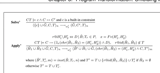
Table 2.1: The transition system T for compositional semantics
℘(A) denotes the powerset set of A. Note that we modify the notion of configuration (Conft) used before by merging the goal store with the CHR store, since we do not need
to distinguish between them. Consequently the Introduce rule is now useless and we eliminate it. On the other hand, we need the information on the new assumptions, which is added as a label to the transitions.
We need some further notation: given a goal G, we denote by ˜G one of the possible identified versions of G. Moreover, assuming that G contains m CHR-constraints, we define a function Inn+m(G) which identifies each CHR constraint in G by associating a unique integer in [n+1, m+n] with it, according to the lexicographic order. The identifier association is applied both to the initial goal store, at the beginning of the derivation, and to the bodies of the rules that are added to the goal store during the computation steps. If m = 0, we assume that In
n(G) = G.
Let us now briefly consider the rules in Table 2.1. Solve’ is essentially the same rule as the one defined in Table 1.3, while the Apply’ rule is modified to consider assumptions: when reducing a goal G by using a rule having head H, the set of assumptions K = H \G (with H 6= K) is used to label the transition. Note that since we apply the function Inn+k to the assumptions K, each atom in K is associated with an identifier in [n + 1, n + k]. As before, we assume that program rules use fresh variables to avoid variable name captures. Given a goal G with m CHR-constraints an initial configuration has the form hIm
0 (G), true, ∅im where I0m(G) is the identified version of the goal.
A final configuration has either the form h ˜G, false, T inif it has failed or h∅, c, T in,
The following example shows a derivation obtained by the new transition system. Example 2.1 Given the goal (C = 7, A =< B, C =< A, B =< C, B =< C) and the program of Example 1.1 by using the transition system of Table 2.1 we obtain the following derivation (where the last step is not a final one):
h{C = 7, A =< B#1, C =< A#2, B =< C#3, B =< C#4}, true, ∅i4→∅ Solve
h{A =< B#1, C =< A#2, B =< C#3, B =< C#4}, C = 7, ∅i4→∅ trs@1, 3
h{A =< C#5, A =< B#1, C =< A#2, B =< C#3, B =< C#4}, C = 7, {trs@1, 3}i5→∅ asx@5, 2
h{A = C, A =< B#1, B =< C#3, B =< C#4}, C = 7, {trs@1, 3}i5→∅ Solve
h{A =< B#1, B =< C#3, B =< C#4}, (A = C ∧ C = 7), {trs@1, 3}i5→∅ asx@1, 3
h{B = C, B =< C#4}, (A = C ∧ C = 7), {trs@1, 3}i5→∅ Solve
h{B =< C#4}, (B = C ∧ A = C ∧ C = 7), {trs@1, 3}i5
The semantic domain of our compositional semantics is based on sequences which represent derivations obtained by the transition system in Table 2.1. We first consider “concrete” sequences consisting of tuples of the form h ˜G, c, T, m, Im+k
m (K), ˜G
0, d, T0, m0i.
Such a tuple represents exactly a derivation step h ˜G, c, T im −→KP h ˜G
0, d, T0i
m0, where k
is the number of CHR atoms in K. The sequences we consider are terminated by tuples of the form h ˜G, c, T, n, ∅, ˜G, c, T, ni, with either c = false or ˜G is a set of identified CHR constraints, which represent a terminating step (see the precise definition below). Since a sequence represents a derivation, we assume that if
. . . h ˜Gi, ci, Ti, mi, ˜Ki, ˜G0i, di, Ti0, m 0 ii
h ˜Gi+1, ci+1, Ti+1, mi+1, ˜Ki+1, ˜G0i+1, di+1, Ti+10 , m0i+1i . . .
appears in a sequence, then ˜G0i = ˜Gi+1, Ti0 = Ti+1and m0i ≤ mi+1hold.
On the other hand, the input store ci+1can be different from the output store di
pro-duced in a previous step, since we need to perform all the possible assumptions on the constraint ci+1 produced by the external environment, in order to obtain a compositional
semantics, so we can assume that CT |= ci+1→ diholds. This means that the assumption
made on the external environment cannot be weaker than the constraint store produced in the previous step. This reflects the fact that information can be added to the constraint store and cannot be deleted from it. The idea is that CT |= ci+1 → di, with ci+1 6= di,
supposes that another sequence, which generates the constraint ci+1\di is inserted, into
a concrete sequence which does not correspond a real computation. Finally, note that assumptions on user-defined constraints (label K) are made only for the atoms which are needed to “complete” the current goal in order to apply a clause. In other words, no as-sumption can be made in order to apply clauses whose heads do not share any predicate with the current goal.
Example 2.2 The following is the representation of the derivation of Example 2.1 in terms of concrete sequences:
h{C = 7, A =< B#1, C =< A#2, B =< C#3, B =< C#4}, true, ∅, 4, ∅ {A =< B#1, C =< A#2, B =< C#3, B =< C#4}, C = 7, ∅, 4i h{A =< B#1, C =< A#2, B =< C#3, B =< C#4}, C = 7, ∅, 4, ∅ {A =< C#5, A =< B#1, C =< A#2, B =< C#3, B =< C#4}, C = 7, {trs@1, 3}, 5i h{A =< C#5, A =< B#1, C =< A#2, B =< C#3, B =< C#4}, C = 7, {trs@1, 3}, 5, ∅ {A = C, A =< B#1, B =< C#3, B =< C#4}, C = 7, {trs@1, 3}, 5i h{A = C, A =< B#1, B =< C#3, B =< C#4}, C = 7, {trs@1, 3}, 5, ∅ {A =< B#1, B =< C#3, B =< C#4}, (A = C, C = 7), {trs@1, 3}, 5i h{A =< B#1, B =< C#3, B =< C#4}, (A = C, C = 7), {trs@1, 3}, 5, ∅ {B = C, B =< C#4}, (A = C, C = 7), {trs@1, 3}, 5i h{B = C, B =< C#4}, (A = C, C = 7), {trs@1, 3}, 5, ∅ {B =< C#4}, (B = C, A = C, C = 7), {trs@1, 3}, 5i h{B =< C#4}, (B = C, A = C, C = 7), {trs@1, 3}, 5, ∅ {B =< C#4}, (B = C, A = C, C = 7), {trs@1, 3}, 5i We then define formally concrete sequences, which represent derivation steps, per-formed by using the new transition system as follows:
Definition 2.1 (Concrete sequences) The set Seq containing all the possible (concrete) sequences is defined as the set
Seq = {h ˜G1, c1, T1, m1, ˜K1, ˜G2, d1, T10, m 0 1ih ˜G2, c2, T2, m2, ˜K2, ˜G3, d2, T20, m 0 2i · · · h ˜Gn, cn, Tn, mn, ∅, ˜Gn, cn, Tn, mni |
for eachj, 1 ≤ j ≤ n and for each i, 1 ≤ i ≤ n − 1, ˜
Gj are identified CHR goals, ˜Ki are sets of identified CHR constraints,
Tj, Ti0 are sets of tokens,mj, m0iare natural numbers and
cj, diare built-in constraints such that
Ti0 ⊇ Ti, Ti+1 ⊇ Ti0, m 0
i ≥ mi, mi+1 ≥ m0i,
CT |= di → ci, CT |= ci+1 → diand
From these concrete sequences we extract some more abstract sequences which are the objects of our semantic domain. If h ˜G, c, T, m, ˜K, ˜G0, d, T0, m0i is a tuple, different from the last one, appearing in a sequence δ ∈ Seq, we extract from it a tuple of the form hc, ˜K, ˜H, di where c and d are the input and output store respectively, ˜K are the assump-tions and ˜H the stable atoms: the restriction of goal ˜G to the identified constraints, that will not be used any more in δ to fire a rule. The output goal ˜G0 is no longer consid-ered. Intuitively, ˜H contains those atoms which are available for satisfying assumptions of other goals, when composing two different sequences, representing two derivations of different goals.
If hci, ˜Ki, ˜Hi, diihci+1, ˜Ki+1, ˜Hi+1, di+1i is in a sequence, we also assume that ˜Hi ⊆
˜
Hi+1holds, since the set of those atoms which will not be rewritten in the derivation can
only increase. Moreover, if the last tuple in δ is h ˜G, c, T, m, ∅, ˜G, c, T, mi, we extract from it a tuple of the form hc, ˜G, T i. We can define formally the semantic domain as follows in the next definition but first we must define the abstract sequences that will be used from now on.
Definition 2.2 (Sequences) The semantic domain D containing all the possible sequences is defined as the set
D = {hc1, ˜K1, ˜H1, d1ihc2, ˜K2, ˜H2, d2i . . . hcm, ˜Hm, T i |
m ≥ 1, for each j, 1 ≤ j ≤ m and for each i, 1 ≤ i ≤ m − 1, ˜
Hj and ˜Kiare sets of identified CHR constraints,
T is a set of tokens, ˜Hi ⊆ ˜Hi+1andci, di are built-in constraints
such thatCT |= di → ciandCT |= ci+1→ dihold}.
In order to define our semantics we need two more notions. The first one is an abstrac-tion operator α, which extracts from the concrete sequences in Seq (representing exactly derivation steps) the sequences used in our semantic domain. To this aim we need the notion of stable atom.
Definition 2.3 (Stable atoms and Abstraction) Let
be a sequence of derivation steps where we assume that the CHR atoms are identified. We say that an identified atom g#l is stable in δ if g#l appears in ˜Gj and the identifier l
does not appear inTj\ T1, for each1 ≤ j ≤ m. The abstraction operator α : Seq → D
is then defined inductively as
α(h ˜G, c, T, n, ∅, ˜G, c, T, ni) = hc, ˜G, T i
α(h ˜G1, c1, T1, n1, ˜K1, ˜G2, d1, T2, n01i · δ0) = hc1, ˜K1, ˜H, d1i · α(δ0).
where ˜H is the set consisting of all the identified atoms ˜h such that ˜h is stable in h ˜G1, c1, T1, n1, ˜K1, ˜G2, d1, T2, n01i · δ
0.
We should point out at this point that the token store does not only keep trace of the application of the rules with empty lhs (left hand side) of \: the one equivalent of the pure simplification rules.
The following example illustrates the use of the abstraction function α.
Example 2.3 The application of the function α to the (concrete) sequence in Example 2.2 gives the following abstract sequence:
htrue, ∅, {B =< C#4}, C = 7i hC = 7, ∅, {B =< C#4}, C = 7i hC = 7, ∅, {B =< C#4}, C = 7i hC = 7, ∅, {B =< C#4}, (A = C ∧ C = 7)i h(A = C ∧ C = 7), ∅, {B =< C#4}, (A = C ∧ C = 7)i h(A = C ∧ C = 7), ∅, {B =< C#4}, (B = C ∧ A = C ∧ C = 7)i
h(B = C ∧ A = C ∧ C = 7), {B =< C#4}, {trs@1, 3}i
Before defining the compositional semantics we need a further notion of compatibility. To this end, given a sequence of derivation steps
δ = h ˜G1, c1, T1, n1, ˜K1, ˜G2, d1, T2, n01i . . . h ˜Gm, cm, Tm, nm, ∅, ˜Gm, cm, Tm, nmi
and a derivation step t = h ˜G, c, T, n, ˜K, ˜G0, d, T0, n0i, we may define Vloc(t) = F v(G0, d) \ F v(G, c, K) (the local variables of t),
Vass(δ) =Sm−1i=1 F v(Ki) (the variables in the assumptions of δ) and
Vloc(δ) =Sm−1i=1 F v(Gi+1, di) \ F v(Gi, ci, Ki) (the local variables of δ, namely the