Cutting the Labor Tax Wedge in Hard Times. Evidence from an Italian Reform

(1)

Fiscal devaluation in hard times.

Evidence from an Italian reform

∗

Massimo Bordignon

Marie-Luise Schmitz

Gilberto Turati

September 15, 2017

Abstract

As first part of a strategy aimed at defining a fiscal devaluation, in 2007, the Italian government implemented a reform reducing the labor tax wedge to boost firms’ competitiveness. In this paper, we provide evidence on the causal impact on employment of this reform using a DDD model and exploiting differences across geographical areas and sectors of economic activity in the tax allowances. Our findings suggest a mildly positive effect of the reform on employment. We interpret this result by observing that the magnitude of the tax incentive was too small for firms to increase the number of workers.

Keywords: fiscal devaluation, labor tax wedge, Italy

JEL Codes: H25, J21, R12

∗

Bordignon: Catholic University of Milan & CESifo Munich (massimo.bordignon@unicatt.it); Schmitz: European Commission, Joint Research Centre, Fiscal Policy Analysis Unit (marie-luise.schmitz@ec.europa.eu); Turati: Catholic University of Milan (gilberto.turati@unicatt.it). The findings, interpretations and conclusions expressed in this paper are entirely those of the authors and should not be attributed to the European Commission. Possible errors and omissions are those of the authors and theirs only.

(2)

1 Introduction

The European economic crisis has impressively revealed the deficiencies of the currency union: in the first half of the 2000’s, large fiscal imbalances have accumulated across member states with diverging paths of productivity and the formation of huge external debts, especially in Southern Europe; in 2007, the international crisis has led to a quick reversal of capital flows across countries, forcing the European Central Bank to take ex-ceptional measures to support the banking system of the most troubled member states. Output losses and increasing unemployment threatened the sustainability of public fi-nances and jeopardized social support for the Euro as a common currency. Given the impossibility of currency devaluations in the Euro area, other solutions had to be found to increase international competitiveness of eurozone countries, especially the Southern ones.

An idea that gained considerable support in the literature and among international organizations has been that of using the tax system to mimic a currency devaluation (EC 2008; IMF 2011; OECD 2013). The policy proposal, known as fiscal devaluation, is based on a tax shift from direct to indirect taxation: governments should reduce taxes on inputs (especially on labor), financing the cut with increases in other taxes, notably value-added taxes and property taxation. With a fixed exchange rate and rigid nominal wages this tax shift would result in increased domestic consumer prices for imports and reduced unit labor cost. Reduced unit labor costs should provide incentives for firms to increase their demand for labor while, on the consumption side, lower producer prices for exported goods should improve the competitiveness of the country vis-à-vis trading partners. The overall effect depends on both the substitutability in consumption of foreign and domestic goods, and on the lag with which nominal wages adjust to the increase in domestic prices induced by the tax shift.

As for Italy, the theoretical requirements to have the desired effects on employment and competitiveness were (and still are) largely satisfied. Italy is among the eurozone

(3)

countries that are most in trouble for the high level of debt and its stifled growth, accord-ing to IMF (2012) the share of exports under a fixed exchange rate was (and still is) quite large (roughly 50% of exported goods and services go to eurozone trading partners), and the trade within the eurozone is significantly more responsive to relative price changes (which would accelerate the reaction of exports and imports in response to a tax shift (Turunen, Harmsen, and Bayoumi 2011). Moreover, a lack of productivity growth and a high tax wedge on labor have raised unit labor costs relative to the eurozone, resulting in a slight over-valuation of about 5-10%. Finally, the country was characterized by significant labor market rigidities (some of them removed with the recent Jobs Act in 2015; see e.g., Sestito and Viviano (2016), hence the advantages from reduced labor tax wedge could materialize in the time between wage negotiations.

Although the theoretical case for fiscal devaluation seems convincing (e.g., Fahri, Gopinath, and Itskhoki (2014), its real-world effectiveness is still an open issue. Nei-ther simulation nor cross-country studies offer clear cut evidence, in addition to being sensitive to different kinds of problems. While the first are able to evaluate the general equilibrium effects stemming from fiscal devaluation but entirely rely on calibration is-sues, the second need to concentrate on specific outcomes and likely suffer bias arising from unobserved country-specific heterogeneity. Recent econometric evidence is offered for instance by De Mooij and Keen (2012), who use an unbalanced panel of 30 OECD countries between 1965 and 2009 to estimate the effect on net exports of changes in the revenues from social security contributions and VAT. In contrast to simulation-based re-search, the estimates suggest significant and quite sizable short run effects for eurozone countries. A tax shift in the order of 1% of GDP is expected to increase net exports by up to 4% of GDP but the effects eventually disappear in the long run. These estimates are, however, subject to substantial endogeneity concerns that usually arise in the context of macro regressions. Unobserved cross-country heterogeneity as well as macroeconomic shocks may be associated with both different levels of taxation and exports resulting in

(4)

misleading causal interpretations.

One main difficulty with the econometric evaluation of the impact of fiscal devaluation is that only few countries really carried out ‘standard’ fiscal devaluations. The most important recent example is that of Germany, which raised VAT from 16 to 19% and cut social security contributions from 6.5 to 4.2% at the same time in 2007. Most of the other European countries introduced separately the cut in the labor tax wedge and the increase in consumption taxes (Puglisi 2014), what one can call a ‘non-standard’ fiscal devaluation. Italy is a case study in this respect: in 2007, the government introduced a reform reducing the labor tax wedge as a first part of a package aimed at implementing a fiscal devaluation to be completed increasing the VAT tax rate in the fall of 2011, and then further in 2013.

Our contribution is focused on the first part of the ‘non-standard’ fiscal devaluation carried out in Italy: we consider a geographically differentiated reform of the Italian regional tax on productive activities (Irap) implemented in 2007 to reduce the labor tax wedge. In particular, we aim at studying the impact of this ‘non-standard’ fiscal devaluation on the labor market, looking for supportive evidence of the theoretical view that fiscal devaluation may improve firms’ competitiveness and, consequently, increase labor demand. Causal evidence on the local average effect of the reform is provided by exploiting the geographical discontinuity introduced by the reform, together with differentiated allowances across different sectors of economic activity. Our results suggest mildly positive effects on employment of the tax reform during the hard times of the economic crisis. Our interpretation is that the fiscal stimulus for each firm was relatively small - allowing a tax saving of only 1.6-2.9% of the average wage at the statutory tax rate – for the tax shift to have significant effects on employment.

The remainder of the paper is structured as follows. Section 2 provides essential back-ground information on the Tax on Productive Activities and the 2007 reform. Section 3 presents the data, while the descriptive evidence on the effects of the reform are in

(5)

Section 4. Section 5 is devoted to identification and estimation issues, while results are discussed in Section 6. Section 7 briefly concludes.

2 Background

2.1 Irap in Italy

The Tax on Productive Activities (Irap, Imposta Regionale sulle Attività Produttive) was implemented by the Prodi’s centre-left government in 1998 as a key piece of a broad reform package aimed at addressing a variety of issues at once. Firstly, in the corporate sector, high statutory tax rates on income and profits as well as a small additional tax on business net worth were deemed to have significant distortive effects, favoring tax evasion and high debt-financing as well as impeding domestic and foreign investment,

and discriminating against corporate legal status.2 Hence, the tax burden was shifted

away from profits towards a broader definition of corporate and non-corporate business income, including for the first time interest payments which had been entirely untaxed until then. Secondly, a persistent situation of regional overspending in the health care sector and repeated bailouts by the national government convinced authorities that providing regions with an autonomous source of revenue would contribute to increase their fiscal accountability by hardening their budget constraints (Bordignon and Turati 2009). Although the tax base is specifically defined according to a firm’s legal form and sector of activity (e.g., different criteria apply to banks, financial intermediaries, farmers, and the public administration), in general terms it equals the difference between the value of production and costs for intermediate goods, services, and write-downs; this difference corresponds to the sum of wages, profits, rents and interest payments. By definition, Irap is then payable also in case of losses, which may aggravate the situation of struggling companies, a fact that has evoked particular criticism since its introduction. Given its

2

See Bordignon, Giannini, and Panteghini (2001) for an extensive assessment of the reform in the corporate sector as well as its evaluation against the European background.

(6)

broad tax base, considerable revenue is obtained at a relatively low ordinary statutory rate: the tax rate was originally set at 4.25% in 1998, and it has been reduced to 3.90% in 2008. Like for the definition of the tax base, specific rates apply to different sectors of economic activity and legal forms; for example, public administrations have been usually subject to increased rates with respect to ordinary rate (at present 8.5%) and farmers to reduced rates (at present 1.9%). The regulations allowing regions to modify the statutory rate, and to differentiate the rate for specific sectors of economic activity were modified several times during the years. The 1998 law initially allowed regions to alter the tax rate up to 1% starting from the year 2000, but in 2003 this possibility was suspended in the absence of any agreements on the structural mechanisms of fiscal federalism (of which Irap was clearly a cornerstone). However, the increase in the tax rate was made compulsory in 2006 for covering deficits in regional health care systems, leading since then to increased rates in the regions Abruzzo, Campania, Lazio, Molise, and Sicilia. Regions not running deficit were set free to choose the rate in 2007, up to 0.92% since 2008, but in 2009 this possibility was blocked again.

2.2 The reform

With the Budget Law for 2007, as a first step towards the implementation of a fiscal devaluation, the Italian legislator introduced a reduction of the labor tax wedge per employee with the declared goal to boost firms’ competitiveness. This newly introduced Scheme 6 (following the classification of deductions for dependent employment by art. 11 of Legislative Decree n. 446/1997 regulating Irap, see table 1) defines an uncondi-tional yearly lump-sum deduction from the tax base of 4,600 e (5,000 e prior to 2008) for each employee with permanent contract as well as the deduction of the entire amount of social security contributions payable by the employer. This deduction is our treatment in the following empirical analysis. Besides the temporal variation, there are two addi-tional sources of exogenous change in the treatment: by geographical area and by sector

(7)

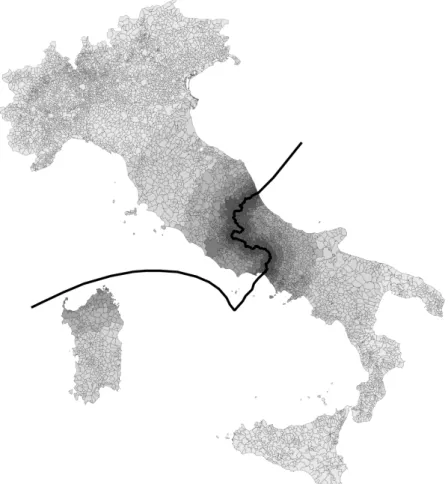
of economic activity. First, the base lump-sum amount is increased to 9,200 e (10,000 e prior to 2008) for firms located in the South of Italy, i.e., in the regions Abruzzo, Basilicata, Calabria, Campania, Molise, Puglia, Sardegna, and Sicilia. Figure 1 illus-trates the geographical differentiation of the treatment and the resulting reform border. Second, economic sectors like the sector of public utilities and the public administration are not granted the deduction across all regions, whereas firms in the financial sector are not granted the differential treatment in Southern regions. According to data pub-lished by the Ministry of Finance, lump sum deductions totaled about 40 billion euro at the national level for each of the years between 2008 and 2010 (data for 2007 are not available) implying a financial stimulus of about 1.5 billion euro (about 1% of GDP)

involving more than a million of firms.3 Unsurprisingly, one fourth of the total value

of these deductions went to firms in Lombardy, the most populated and richest region in Italy, approximately the same value for all the Southern regions considered together: this clearly reflects the uneven distribution of economic activities in the country, which makes comparison at the national level hard to be made. However, looking at regions closer to the border (Umbria, Marche and Lazio in the North; Abruzzo, Molise and Cam-pania in the South) this picture rapidly changes: both the total amount and the number of firms get closer between the two sides of the border, and the average deduction is now larger for Southern firms (38,000 euro for 2008) than for Northern ones (36,000 euro for the same year), generating a fiscal advantage - given the tax rate - of about 1,500 euro versus 1,400 euro for firms located on different sides of the boundary. This is not the only deduction scheme, however. Table 1 gives a complete picture of all the deductions for dependent labor implemented before 2007 when Scheme 6, the reform under scrutiny here, started. Alternative schemes from 1 to 4 consider for instance deduction of the employers’ compulsory unemployment insurance contributions irrespective of the type of labor contract in force (i.e., permanent or fixed-term, full or part-time contracts) or

3

(8)

the entire labor cost for apprentices, disabled employees, and R&D workers. Deductions cannot be cu- mulated but for Scheme 1, under the obvious general condition that the total amount to deduce does not exceed labor cost. Most important for our analysis, they are available across the whole country. On the contrary, Scheme 5 exhibits signif-icant spatial as well as temporal variation. It is intended to target employment with permanent contracts and is operative from 2005 to 2008, when the deduction expires. It covers both full and part-time permanent contracts but it is conditional on the effective increase of a firm’s workforce, allowing for the deduction of labor costs up to a limit of 20,000 e for each newly employed if the average number of permanent workers has been increased with respect to the previous year. An increase of the occupational level is realized if the difference between employees at the end of a year and the average number of employees in the previous year is positive, irrespectively of total wages paid. Since 2005, the base deductible amount triplicated in low support areas (LSA) and quintupled in high support areas (HSA) for firms located in economically weak municipalities in accordance with European regulation on the authorization for State aid; furthermore, since 2007, it is quintupled (LSA) or multiplied by seven (HSA) for newly hired female employees in the respective areas. For our identification strategy, it is crucial to recog-nize that LSA and HSA does not match the simple North-South divide characterizing Scheme 6. Despite offering much larger deductions with respect to Scheme 6, Scheme 5 was used by a smaller number of firms (about 110,000), implying reduced revenues of about 5.5 billion euro. The reason is that Scheme 5 was more risky than Scheme 6, especially in difficult times, since the tax allowance had to be given back if the labor force was reduced in the next three years.

2.3 Hypothesis

The expected effects of the tax reform can be analyzed by looking at what the allowances introduced by Scheme 6 really mean for firms located at the North and the South of the

(9)

border. Table 2 reveals that the economic advantage for an individual firm is relatively small. We consider 2007 annual average wages of about 21,000 euro and 31,000 euro for blue and white collars respectively, and compute the tax savings at the statutory Irap rate for a firm hiring a new worker with a permanent contract at the beginning of the year. Social security contributions allow a saving of 209 (306) euro for each blue (white) collar, while the lump sum deduction results in a further saving per worker of 212 euro if the firm is located north to the border, compared to 425 euro if the firm is located south of the border. To put it differently, the Irap Scheme 6 reform allows firms to save 1.9% (1.6%) and 2.9% (2.3%) per each new blue (white) collar with a permanent contract, for Northern and Southern firms respectively. In deciding whether or not to hire a new worker with a permanent contract, or to transform a temporary contract into a permanent one, we expect this small incentive to have had rather small effects on total employment. In particular, in hard times like those characterizing the reform period, the incentive could have been used to maintain current employment (or to reduce layoffs) as a response to shrinking profits. Perhaps this should be recognized as a positive impact of the reform.

3 Data

As plant or firm level data for dependent employment are not available, in order to assess the effects of the 2007 tax experiment, we assembled municipal employment data with a set of local controls, and a measure of geographical distance to the reform border. In particular, we rely on the Statistical Register of Active Enterprises (ASIA) provided by the Italian National Institute of Statistics (Istat), which contains the number of firms, plants, and employees across 12 sectors of economic activity for all Italian municipal-ities in the period 2005-2010. Wage bill data are not available at the municipal level, which makes it impossible to quantify the effect of the tax cut on wage adjustment and to study its potentially dampening effect on labor demand. Our focus is on the total

(10)

number of full-time equivalent employees in each municipality . Unfortunately, we do not have information on the type of labor contract involved (temporary or permanent, part- or full-time), which eventually makes even more challenging to identify a positive impact of the reform (extensive vs. intensive margin). In fact, we are unable to measure if employers transform existing temporary contracts into permanent ones in order to become eligible for the new deduction (e.g., to change from Scheme 4 to Scheme 6), or if they increase hours of work for present employees (the intensive margin). The analysis is restricted to the potential occurrence of new hires in addition to the existent work-force as a result of the reform, irrespectively of the type of labor contract that is being used (the extensive margin). Additionally, employees are assigned to municipalities ac-cording to firms active in each municipality, and not their residence. Hence, for some municipalities, it is possible to have the number of employees higher than the number of people living in that particular municipality, which makes it difficult to compute a municipal employment rate. To avoid this problem, we compute an employment index (EMPL) for each municipality and each sector of economic activity, taking 2005 as the

base year.4 _{In order to account for the geographical discontinuity underlying the reform}

illustrated in Figure 1, we use the geographical information system ArcGIS to obtain the perpendicular distance of a municipality’s border to the border separating target and comparison areas. In this way, municipalities at the border have a distance equal to zero. Before moving further notice that we excluded from our analysis municipalities in the region Sardinia as well as the municipality of Rome, given the peculiar nature of the labor markets in both areas. Also notice that this very simple North-South divide defined in Scheme 6 is also different from classifications of municipalities in high or low

support area as defined by Scheme 5 (HSA, LSA).5 Figure 2 illustrates the evolution of

4_{We excluded all instances in which in some sectors in particular municipalities, employment was zero.} We also excluded outliers following standard procedures.

5_{See the Ministerial Decree 27/03/2008 for the list of areas admitted to state aid in the period} 2007-2013 and the Appendix of Circular 32/E, 03/06/2003 of the Revenue Agency for the respective areas in the period 2000-2006.

(11)

the index in six macro sectors of economic activity averaging over Northern and Southern municipalities located within a range of 100 km from the border. Overall the evolution of the average employment index is quite similar between the two areas of the country, and shows the hard times characterizing the reform period. Between 2005 and 2007, the Northern and the Southern municipalities follow the same positive trend with the Northern area performing slightly better on average. In both areas, the index raises to above 104 in 2008, and then declines sharply following the evolution of the crisis, down to 102 in Northern and to 101.6 in Southern municipalities, respectively. However, the overall average hides important differences. We therefore define six macro sectors of economic activity instead of the original twelve in order to avoid having sectors with zero employees: manufacturing (including manufacturing and extraction), construction, services (including wholesale and retail trade, accomodation and food services activities, real estate activities), utilities (electricity, gas and water supply, sewerage and trans-ports), finance (including financial and insurance activities), and collective (or public) services (including most of the public administration in education and health care, but also other services like theaters and cinema mostly provided by private firms). Disaggre-gated by macro-sectors, it is evident that the manufacturing sector is the one suffering most from the economic crisis: for both North and South, it shows a steady decline, down to less than 92 for Northern municipalities and to about 93 for Southern ones; interestingly, the decline for Southern municipalities appears to be less severe than for Northern municipalities as of 2007, when the reform kicks in (see Figure 2). The evolu-tion in the construcevolu-tion, services and utilities sectors resemble the overall average across sectors: the index increases up to 2007-2008, and then declines. The decline is large for the construction sector, with employment getting almost back to the 2005 value both in the North and in the South, after a peak of 108 in 2007, which marks a peak also of transactions (and prices) in the housing market. The decline is less pronounced for the services sector where it is also less marked for Southern than for Northern

(12)

munici-palities. A completely different pattern characterizes finance and the collective services sectors, among those excluded (or partially excluded) from the reform. The financial sector marks an increase of about 5 percentage points in both areas, while for collective services we observe a larger increase for Northern municipalities compared to Southern ones.

4 Descriptive evidence on the effects of the reform

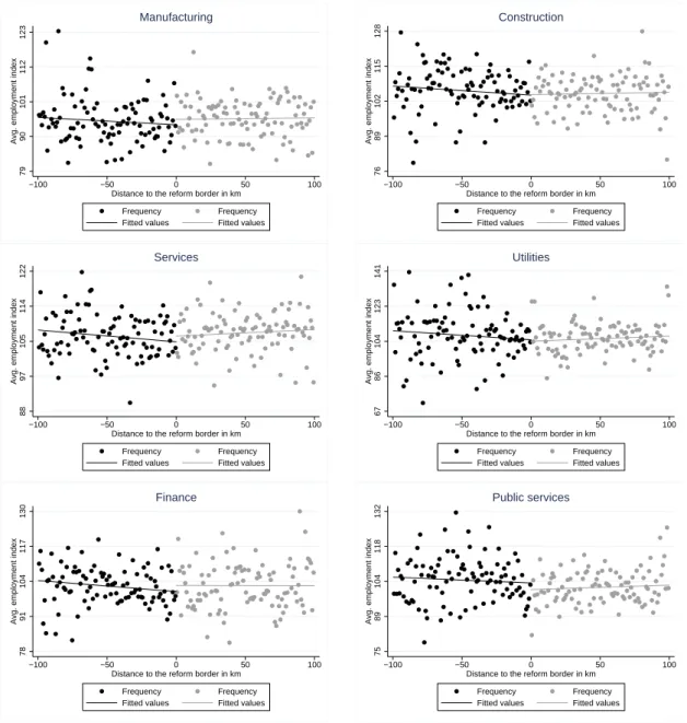
Figure 3 reports the average employment index for the 2007-2010 post-reform period by macro sectors for all municipalities within 100 km to the reform border. The distance to the border is transformed into an ‘assignment’ variable with negative values to the North, and positive values to the South of the border. There are no evident discontinuities at the border, which suggests that the reform produced at best modest effects in terms of employment. We run the same exercise for all the six macro-sectors. Evidence of small discontinuities at the border seems to emerge for the manufacturing, services and financial sectors in favor of Southern municipalities, while they are in favor of Northern municipalities for collective services.

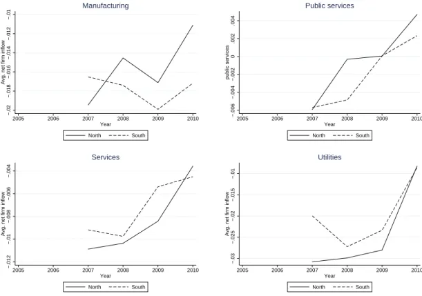
To be sure that what we observe can be attributed to the reform, we need to verify that prior to the introduction of the reform there were no discontinuities at the border. We therefore consider the same exercise of Figure 3 only for the year 2006 (Figure 4), again starting from the average over all sectors and then separately for the six macro sectors. With the exception of finance and collective services, there emerge small dis-continuities around the border in favor of Southern municipalities; but these differences are never statistically significant when testing discontinuities using confidence interval estimators provided by Calonico et al. (2014). An additional concern is related to the possibility that, given the reform, firms decide to manipulate their location across the border in order to exploit the advantages introduced for firms located in the South. To exclude this possibility we verify whether we observe a differential flow of firms on the

(13)

two sides of the border after the reform has been implemented. As municipal data are unavailable, we consider provincial data obtained from the Italian Chambers of Com-merce (Movimprese). There are 12 provinces on either side of the border within the range of 100 km. Net firm inflow is defined as the difference of inscribed and stopped firms in a given year, standardized by the number of registered firms in the previous year. Figure 5 shows the net firm inflow in the post-reform period in the Southern and the Northern area, respectively. If anything, firm inflow was higher in Northern provinces

with respect to Southern ones across all the years.6

A final issue is about the comparability of municipalities across the two sides of the border in the pre-treatment years. We tested comparability at different distances from the border (from zero to 100 km) with a t-test, considering employees, plants and firms in the year 2005, taking into account all sectors and then separately the six macro-sectors. We also tested for some structural characteristics of municipalities, like population, the age composition of the population, the area and the degree of urbanization. The general message from Table 3 is that municipalities within the range of 100 km are largely comparable before the introduction of the reform. At 100 km from the border, only the number of plants and firms in the construction sector seems to be statistically different between municipalities on the two sides of the border. The other differences that emerge are in terms of municipalities’ area and the degree of urbanization; but both variables do not seem to affect the conclusions of our analysis.

5 Identification and estimation

Our goal is to measure the discontinuity in the employment index at the assignment threshold, which corresponds here to the border between treated Southern regions and Northern ones, accounting for a different treatment also across sectors of economic

ac-6_{In addition, we tested for differences in means for each macro sector. The test indicates a significant} difference in average net firm inflow for the financial sector with the north experiencing a negative inflow and the South a slightly positive inflow.

(14)

tivity. The use of allowances introduced by the tax reform was of course optional for firms. However, our analysis here considers six macro-sectors of economic activity for each municipality as unit of observation; and for each of these we computed our index EMPL. We then assume that all sectors and municipalities in the treated regions did receive the treatment. In this sense, we have a sharp regression discontinuity design, and the discontinuity identifies the average causal effect of the reform for different neighbor-hoods from the border. The validity of this identification strategy has been discussed in the previous section. First, we showed that there were no statistically significant discontinuities at the border in the index EMPL prior to the introduction of the reform. Second, we provide evidence that firms located close to the border did not manipulate their location to exploit the additional advantages introduced for firms located in South-ern regions, after the reform has been implemented. Third, we discuss the comparability of municipalities on the two sides of the border, showing that results cannot be due to differences across the two groups of treated and controls. To identify the impact of the reform we consider in particular the following Diff-in-Diff-in-Diff model:

EM P Ljit=β₁d06S_j+β₂R_tS_j+β₃R_tS_jG_i+δX + φD_{Y t}+γD_Gi+ϕD_Sj+ε_jit

where: d06 identifies a dummy for the year 2006; R identifies the tax reform dummy, equal to one from 2007 onwards; S identifies a dummy for the treated sectors (manu-facturing, services and construction); G identifies a dummy for treated regions; X is a

vector of covariates; DY, DG, and DS provide a full set of fixed effects for time, space,

and sectors of economic activity; ε is the disturbance term. The model is estimated con-sidering treated and comparison municipalities within arbitrarily small neighbourhoods of the reform border (N = 0 km, 10 km, 25 km, 50 km, and 100 km). Our coefficient

of interest is β3: a positive coefficient identifies a positive causal impact of the reform

(15)

between the reform dummy and the treated sectors allows to test for the presence of different trends across these sectors after the reform, while the interaction between the dummy d06 and the treated sectors allow to test for the presence of different trends across these sectors prior to the reform.

As for space fixed effects DG, we consider the Labour Market Areas (Sistemi Locali

del Lavoro,literally ‘Local labor systems’) defined by Istat as sub-regional geographical

areas where the bulk of the labour force lives and works, and where establishments can find the largest amount of the labour force necessary to occupy the offered jobs. The definition is based on the analysis of commuting patterns and LMAs are not designed to respect administrative boundary constraints, so that they can stretch across two different regions. That is why we also include a control for border-crossing LMAs, identifying treated and untreated municipalities that share a common area of commuting workers. The vector X includes both a set of local controls, as well as a set of dummy variables to control for confounding Irap alternative schemes. Among local controls we consider: the Irap rate, which can be differentiated across regions, and provide different incentives for firms; a dummy indicating whether the region is under a recovery plan for excessive deficits (the so-called ‘Piano di Rientro’) in health care, the function typically managed at the regional level in Italy; the size of the municipality in terms of population; the share of citizens older than 65 in 2001 to account for the non-working population, which works also as a municipal fixed effect. We address the problem of confounding Irap schemes by including a set of dummy variables indicating whether a municipality belongs to the high or low support area as defined by Scheme 5 (HSA, LSA). As the deductible amount was in turn multiplied for female employees in the respective areas in the period 2007-2008, we further link HSA and LSA with both years in order to account for potential gender effects (HSA female, LSA female). Moreover, while HSAs capture the entire territory of several regions in the South, LSAs are defined at the municipal and sub-municipal level for economically weak areas with high unemployment throughout the country. Therefore,

(16)

we additionally interact LSA with a dummy indicating municipalities to the south of the border in order to distinguish the effect of Scheme 5 for either side of the border. Finally, to account for the likely correlation of the error term for municipalities belonging to the same LMA in the same year, we cluster standard error at both LMA and year level.

6 Econometric results

Estimates of our econometric model are in tables 4 and 5 for the whole sample including all the LMAs. The model has been estimated for five different distances from the border (from zero to 100 km), including the full set of controls, plus time and spatial fixed effects (not reported in the tables, but available upon request from the authors). We consider four groups of estimates depending on the sectors of economic activity used as control groups in the empirical exercise: in the first group, all untreated sectors are used as controls; in the second group, we use only finance and utilities; in the third, we use only public services and utilities; in the last fourth group, we limit controls to public services only. The picture emerging from the analysis is quite consistent across different groups of regressions, and different distances from the border: almost all interaction coefficients for the treated sectors in the post-reform period in the South, albeit positive, are not statistically significant at the usual conventional level. Hence, Scheme 6 does not seem to have produced any differential positive effect on employment in treated areas. One way to interpret this result is related to the tax saving accruing to firms (table 2), too small to really increase employment, especially during these hard times. As for the other coefficients reported in the tables, it emerges clearly that most of the negative effects of the economic crisis have been concentrated in the manufacturing sector: the negative trend is evident starting from 2006, and continues in the post-reform period. If any, the Irap reform helped Southern regions to keep the distances unchanged with respect to Northern regions. Furthermore, there is some evidence supporting the view of a positive trend in employment in the services sector, in both areas, again starting

(17)

before the reform. However, this result vanishes when considering public services only as controls.

One problem with grouping all LMAs together is that some LMAs are crossing the border. In these areas, one might think that labor reallocation across the border would be easier than in non-crossing LMAs, since – differently from administrative boundaries – these take into account commuting patterns of workers. Following this reasoning, we should expect a stronger effect of the reform when considering border crossing local labor systems with respect to no border-crossing LMAs. We then re-estimate our DDD model on two separate sub-samples, one considering only no border crossing LMAs (tables 6 and 7) and the second considering border-crossing LMAs (tables 8 and 9). Results are not very different from estimates including all LMAs, although we do find some evidence now of a positive effect of the reform in the South, but when considering local labor systems completely separate between north and south. This positive and statistically significant effect is limited to manufacturing, and it emerges considering a neighborhood between 25 and 100 km from the border; the effect is still positive but not statistically significant when considering finance and utilities as controls. The magnitude is between 2 and 3.8 points: as the employment index in manufacturing in the South was slightly below 100 when the reform kicks in, these can be directly interpreted as percentage points in the differential trend between South and North municipalities caused by the Irap Scheme 6 reform. Notice that evidence on the negative performance of manufacturing is confirmed. Hence, the reform has helped Southern regions to better limit the negative impact of the economic crisis on employment. Our findings of mildly positive effects (at best) of the tax reform are in line with results from a literature studying the impact of regionally differentiated tax reforms on employment and wages. A number of Scandinavian studies examine the impact of payroll-tax reductions on employment and wages using rich firm or plant level data (e.g., Bohm and Lind (1993), Johanson and Klette (1997), Benn-marker, Mellander, and Öckert (2008), and Korkeamäki and Uusitalo (2008)). However,

(18)

differently from the Italian reform, which aimed at improving firms’ competitiveness in the spirit of a fiscal devaluation, the declared policy objective of these tax cuts was to boost employment in structurally weak regions with high unemployment. Within the target regions, payroll-tax reductions were granted across-the-board, without additional targeting on particular types of labor contracts or low-wage workers. All studies make economic sector considerations with the focus being mostly on manufacturing. Employ-ment is typically captured in terms of the total number of employees per firm or plant whereas wages are defined in terms of gross wage bill or hourly wage. In a nutshell, none of the studies using employment as outcome find significant positive effects, although the tax cut in the two Swedish reforms was sizable, amounting to 10 percentage points of pay-roll taxes (Bohm and Lind 1993; Bennmarker, Mellander, and Öckert 2008). In their analysis of the Finnish experiment, Korkeamäki and Uusitalo (2008) follow the argument that labor demand may be more responsive for low-wage profiles and allow treatment effects to vary for different quartiles of the average wage distribution. Though, they cannot identify any clear-cut pattern. However, contrary to employment, there is evidence that payroll-tax reductions led to significant wage increases, an issue we cannot address for the Italian case. Rescaled to a labor cost reduction in the order of 1%, wages increase in the range of 30-60% of the reduced cost, a magnitude in line with theoretical reasoning. As a result, given the lack of positive labor employment effects, this suggests that employers’ treat the remaining 40-70% of the cost reduction as windfall gain to increase the profit margin. Given the lack of significant increase in the number of em-ployees, something similar could have happened also for Italian firms as a response to the Irap Scheme 6 reform.

7 Conclusions

In this paper we provide evidence on the causal impact on employment of a reform reducing the labor tax wedge, which has been implemented by the Italian government

(19)

in 2007 as a first part of a strategy aimed at defining a fiscal devaluation. Using a DDD model and exploiting differences across geographical areas as well as sectors of economic activities in the tax savings, our findings suggest a mildly positive effect of the reform on employment. The lack of a significant increase in the number of employees – which, according to theory, should be originated by the boost in competitiveness stemming from the fiscal devaluation – is likely to be related to the magnitude of the tax incentive: allowing a saving of less than 3% of the average wage is a too small incentive for firms to increase their employment, especially during hard times like those during which the ‘non-standard’ fiscal devaluation has been implemented. Unfortunately, given our data, we are unable to check whether firms transformed temporary contracts into permanent ones, which would be a positive effect of the reform in the absence of a significant increase in the number of employees.

Our analysis is clearly not looking at the general equilibrium effects of a fiscal deval-uation, but it just concentrates on the impact that the tax shift produced on the labor market. Still, the evidence provided here supports the view that fiscal devaluation might be a policy that can be used in a federation to boost competitiveness of slowly growing countries when currency devaluation is unavailable as a policy tool. However, to have the desired effects on employment, the tax cut on the labor tax wedge must be substan-tial and provide a sizable incentive to firms. Moreover, like for currency devaluation, for these effects to be persistent also in the long run, countries need to remove the structural features of the economy underlying weak growth and competitiveness. Identifying and removing these characteristics is the true challenge for eurozone countries for the years to come.

(20)

Tables and figures

(21)

Table 1: Deductions for dependent employment (Art. 11 Legislative Decree 446/1997)

Year Scheme 1 Scheme 2 Scheme 3 Scheme 4 Scheme 5 Scheme 6

1998 Employers’ obligatory unemploy-ment insurance contributions Labour costs for apprentices (since 1998), disabled em-ployees (since 1999), and staff in charge of research and development activities (since 2005). 1999 2000 2001 2002 2003 Lump-sum deduction of 1,850 € for employees with temporary or permanent contract up to a limit of five employees; eligible are firms with a maximum net value added of 400,000 € 2004 Labour costs for returned researchers 2005 Labour costs up to 20,000 € for each newly employed per-manent worker if average per-manent em-ployment is increased with respect to the previous year. 2006 2007 Lump-sum deduction of 4,600 € (9,200 €) for employees with permanent contract and total amount of employers’ social securtity contributions 2008 2009 2010

(22)

Table 2: Effective annual tax incentive by Scheme 6 (euro by employee)

Northern regions Southern regions

Sector of economic activity SSC lump-sum % wage lump-sum % wage

A) Blue collar

Manufacturing, services, construction 209 212 1.9 425 2.9

Finance 209 212 1.9 212 1.9

Public services, utilities 0 0 0 0 0

A) white collar

Manufacturing, services, construction 306 212 1.6 425 2.3

Finance 306 212 1.6 212 1.6

Public services, utilities 0 0 0 0 0

Notes. Computations are based on average wages for 2007 and rates for SSC provided by INPS and the Irap statutory tax rate.

Figure 2: Average employment index by geographic area and macro sectors, 2005-2010

100

101

102

103

104

Avg. employment index

2005 2006 2007 2008 2009 2010 Year

North South

(23)

Figure 2: (cont) Average employment index by area and macro sectors, 2005-2010 92 94 96 98 100

2005 2006 2007 2008 2009 2010 Year North South Manufacturing 100 102 104 106 108

2005 2006 2007 2008 2009 2010 Year North South Construction 100 102 104 106 108

2005 2006 2007 2008 2009 2010 Year North South Services 100 102 104 106 108 110

2005 2006 2007 2008 2009 2010 Year North South Utilities 98 100 102 104 106

2005 2006 2007 2008 2009 2010 Year North South Finance 98 100 102 104 106

2005 2006 2007 2008 2009 2010 Year

North South

(24)

Figure 3: Average employment index by distance to the border, 2007-2010 87 94 102 109 116

−100 −50 0 50 100

Distance to the reform border in km Frequency Frequency Fitted values Fitted values

(25)

Figure 3: (cont.) Average employment index by distance to the border, 2007-2010 79 90 101 112 123

−100 −50 0 50 100

Manufacturing 76 89 102 115 128

−100 −50 0 50 100

Construction 88 97 105 114 122

−100 −50 0 50 100

Services 67 86 104 123 141

−100 −50 0 50 100

Utilities 78 91 104 117 130

−100 −50 0 50 100

Finance 75 89 104 118 132

−100 −50 0 50 100

(26)

Figure 4: Average employment index by distance to the border, 2006 87 92 97 102 107

−100 −50 0 50 100

All sectors 67 81 95 108 122

−100 −50 0 50 100

Construction 68 81 93 106 118

−100 −50 0 50 100

(27)

Figure 4: (cont.) Average employment index by distance to the border, 2006 75 88 101 114 127

−100 −50 0 50 100

Manufacturing 67 83 98 114 129

−100 −50 0 50 100

Public services 87 93 99 105 111

−100 −50 0 50 100

Services 76 87 98 108 119

−100 −50 0 50 100

(28)

Figure 5: Average net firm inflow, 2007-2010

−.01

0

.01

.02

Avg. net firm inflow

2005 2006 2007 2008 2009 2010 Year North South Construction −.01 0 .01 .02

2005 2006 2007 2008 2009 2010 Year North South Construction −.02 0 .02 .04

2005 2006 2007 2008 2009 2010 Year

North South

(29)

Figure 5: (cont.) Average net firm inflow, 2007-2010 −.02 −.018 −.016 −.014 −.012 −.01

2005 2006 2007 2008 2009 2010 Year North South Manufacturing −.006 −.004 −.002 0 .002 .004 public services 2005 2006 2007 2008 2009 2010 Year North South Public services −.012 −.01 −.008 −.006 −.004

2005 2006 2007 2008 2009 2010 Year North South Services −.03 −.025 −.02 −.015 −.01

2005 2006 2007 2008 2009 2010 Year

North South

(30)

Table 3: T-test of differences in means, North-South, pre-treatment year 2005

0 km 10 km 25 km 50 km 100 km Italy

North South Diff. P-value North South Diff. P-value North South Diff. P-value North South Diff. P-value North South Diff. P-value North South Diff. P-value

All secors Employees 1542.17 1198.02 344.15 0.6169 1037.62 1155.55 −117.93 0.7453 1068.45 912.28 156.17 0.5160 1647.56 1743.28 −95.72 0.8705 1921.85 1618.48 303.37 0.4317 2348.47 1487.22 861.25 0.0159 Plants 490.36 339.62 150.74 0.4546 330.91 355.05 −24.14 0.8209 344.63 290.41 54.22 0.4442 510.24 561.21 −50.96 0.7749 570.29 536.75 33.55 0.7725 622.73 516.17 106.56 0.2674 Firms 448.77 308.62 140.16 0.4438 303.20 324.86 −21.66 0.8236 316.19 266.58 49.61 0.4428 467.95 519.58 −51.63 0.7564 521.81 497.36 24.44 0.8212 567.68 478.08 89.60 0.3172 Manufacturing Employees 374.89 436.28 −61.39 0.7309 285.17 375.50 −90.33 0.3828 290.43 288.49 1.94 0.9779 468.21 383.55 84.66 0.3469 549.20 382.71 166.49 0.0110 693.48 309.16 384.32 0.0000 Plants 53.92 46.23 7.69 0.7066 37.97 45.97 −8.00 0.4641 38.81 36.70 2.10 0.7762 62.39 59.28 3.11 0.8405 70.37 60.65 9.72 0.3434 80.05 57.59 22.45 0.0015 Firms 47.64 39.53 8.11 0.6559 33.42 39.96 −6.54 0.5006 34.17 32.12 2.05 0.7538 55.30 52.59 2.71 0.8489 62.39 53.94 8.44 0.3683 70.32 51.77 18.55 0.0039 Services Employees 651.36 430.28 221.08 0.4841 419.33 445.56 −26.23 0.8723 435.06 352.91 82.15 0.4444 673.66 755.78 −82.13 0.7785 769.16 699.19 69.97 0.7123 981.33 670.08 311.25 0.1045 Plants 285.04 186.02 99.02 0.4130 190.17 199.87 −9.70 0.8798 197.63 164.03 33.60 0.4321 290.54 344.15 −53.61 0.6541 321.66 327.50 −5.84 0.9399 350.33 313.54 36.78 0.5561 Firms 264.83 173.02 91.81 0.4066 177.08 186.67 −9.59 0.8705 184.43 153.91 30.51 0.4390 270.60 324.89 −54.29 0.6328 298.80 309.34 −10.54 0.8857 324.02 295.80 28.22 0.6316 Construction Employees 207.23 139.55 67.67 0.3971 136.57 136.23 0.34 0.9934 141.73 116.34 25.40 0.3401 200.42 203.60 −3.18 0.9471 226.26 190.76 35.50 0.2692 233.95 193.92 40.03 0.1178 Plants 65.98 50.70 15.28 0.5531 45.93 49.64 −3.71 0.7802 48.75 41.13 7.62 0.3829 69.98 62.17 7.81 0.5087 79.67 58.45 21.22 0.0101 84.69 60.05 24.64 0.0013 Firms 62.43 47.66 14.77 0.5407 43.57 46.77 −3.20 0.7974 45.94 38.73 7.21 0.3778 65.59 57.63 7.95 0.4541 74.88 54.26 20.62 0.0059 79.63 55.76 23.87 0.0008 Finance Employees 44.25 26.98 17.27 0.5022 25.35 30.94 −5.59 0.6900 27.64 22.37 5.26 0.5617 43.89 48.27 −4.38 0.8450 51.38 40.93 10.45 0.4786 84.56 39.87 44.69 0.0664 Plants 10.51 6.62 3.89 0.4522 6.62 7.03 −0.41 0.8842 7.36 5.31 2.05 0.2908 11.26 11.07 0.19 0.9661 13.02 10.12 2.90 0.3343 14.48 9.33 5.15 0.0387 Firms 7.15 4.38 2.77 0.4476 4.45 4.62 −0.17 0.9338 5.00 3.41 1.60 0.2531 7.90 7.70 0.20 0.9515 8.82 7.08 1.74 0.4288 9.51 6.23 3.28 0.0735 Utilities Employees 123.55 65.47 58.08 0.2701 81.36 69.31 12.05 0.6738 84.42 54.82 29.59 0.1417 122.56 180.78 −58.22 0.5377 170.97 150.49 20.48 0.7582 179.90 130.84 49.06 0.2372 Plants 20.62 12.68 7.94 0.2586 14.36 12.41 1.95 0.5901 15.19 10.66 4.54 0.0846 20.96 20.13 0.83 0.8987 24.34 20.38 3.97 0.3586 26.98 19.78 7.21 0.0591 Firms 16.15 8.77 7.38 0.1854 11.20 8.75 2.45 0.3973 11.94 7.52 4.42 0.0384 16.63 15.54 1.09 0.8375 19.31 16.00 3.31 0.3463 21.93 15.63 6.30 0.0547 Public administration Employees 141.06 99.51 41.55 0.5404 90.17 98.34 −8.17 0.8175 89.54 77.65 11.89 0.6014 139.29 171.70 −32.41 0.5987 155.36 154.88 0.48 0.9905 175.71 143.79 31.92 0.3983 Plants 54.28 37.36 16.92 0.5009 35.85 40.13 −4.28 0.7511 36.89 32.59 4.30 0.6172 55.11 64.41 −9.31 0.6651 61.24 59.66 1.57 0.9107 66.20 55.88 10.32 0.4386 Firms 50.57 35.26 15.31 0.5160 33.48 38.09 −4.61 0.7175 34.71 30.89 3.82 0.6393 51.94 61.24 −9.30 0.6519 57.62 56.74 0.87 0.9481 62.26 52.89 9.37 0.4650 Population 6101.06 4458.19 1642.87 0.4611 4419.08 4567.67 −148.59 0.9009 4799.23 3914.92 884.31 0.2901 6825.64 8237.66 −1412.03 0.5513 7388.79 8139.44 −750.65 0.6233 6839.69 8123.77 −1284.08 0.1771 Population < 25 1167.34 850.31 317.02 0.4373 846.07 883.46 −37.39 0.8621 877.41 738.14 139.28 0.3179 1187.72 1250.25 −62.54 0.8673 1349.87 1230.47 119.41 0.6237 1321.35 1306.97 14.38 0.9387 Population > 65 1577.61 1136.12 441.49 0.4289 1145.30 1169.05 −23.75 0.9377 1236.02 1036.22 199.80 0.3534 1692.46 2513.00 −820.53 0.2641 1767.00 2516.86 −749.86 0.1109 1487.06 2450.98 −963.93 0.0000 Area city 50.64 62.54 −11.91 0.2931 40.18 52.08 −11.90 0.0599 36.52 42.91 −6.39 0.0800 39.97 32.85 7.13 0.0050 47.39 28.97 18.42 0.0000 32.21 48.12 −15.91 0.0000 Urbanisation 1.36 1.17 0.19 0.0544 1.38 1.25 0.13 0.0539 1.41 1.27 0.15 0.0019 1.51 1.48 0.03 0.4806 1.50 1.68 −0.17 0.0000 1.65 1.49 0.16 0.0000 Degree Observations 53 47 132 100 267 196 446 446 630 848 5540 2554

(31)

Table 4: Effect of the tax experiment on municipal employment index, all local labour systems

All untreated sectors as controls Finance and Utilities as controls

Distance to border 0 km 10 km 25 km 50 km 100 km 0 km 10 km 25 km 50 km 100 km

Manufacturing 2006 -3.726∗∗∗ -1.731∗∗∗ -2.060∗∗∗ -2.087∗∗∗ -1.988∗∗∗ -2.699∗∗∗ -1.051 -1.288∗∗ -1.370∗∗∗ -0.998∗∗∗

(0.936) (0.654) (0.442) (0.287) (0.212) (0.952) (0.701) (0.505) (0.355) (0.244)

Manufacturing post-reform -9.167∗∗∗ -8.503∗∗∗ -8.799∗∗∗ -9.748∗∗∗ -9.359∗∗∗ -7.958∗∗∗ -9.144∗∗∗ -8.778∗∗∗ -9.991∗∗∗ -9.628∗∗∗

(2.879) (2.040) (1.372) (1.713) (1.823) (2.938) (2.221) (1.410) (1.619) (1.640)

Manufacturing post-reform, south 2.056 1.369 2.352 1.870 1.698 -0.0183 0.467 1.432 0.942 0.767

(3.522) (2.357) (1.710) (1.231) (1.105) (3.640) (2.419) (1.921) (1.276) (1.232)

Services 2006 -0.119 1.979∗∗∗ 1.759∗∗∗ 1.313∗∗∗ 1.362∗∗∗ 0.977 2.679∗∗∗ 2.535∗∗∗ 2.039∗∗∗ 2.351∗∗∗

(1.117) (0.691) (0.407) (0.344) (0.243) (1.271) (0.742) (0.485) (0.378) (0.269)

Services post-reform 0.972 3.766∗∗∗ 2.954∗∗ 1.853∗ 2.171∗∗ 1.945 3.130∗∗ 2.959∗∗ 1.628∗ 1.906∗∗

(1.712) (1.261) (1.342) (1.023) (0.874) (1.658) (1.444) (1.483) (0.969) (0.905)

Services post-reform, south 2.629 -0.334 1.928 1.432 1.637 0.851 -1.259 1.042 0.497 0.722

(2.279) (1.408) (1.963) (1.375) (0.997) (2.130) (1.490) (2.129) (1.409) (1.095)

Construction 2006 -1.649 1.072 1.787∗∗ 1.187∗∗ 1.357∗∗∗ -0.653 1.730∗ 2.525∗∗∗ 1.904∗∗∗ 2.339∗∗∗

(1.894) (1.026) (0.771) (0.501) (0.344) (1.859) (0.949) (0.748) (0.545) (0.364)

Construction post-reforms -2.277 0.673 1.510 1.286 1.675 -1.321 0.0170 1.506 1.051 1.399

(2.105) (1.795) (2.050) (1.831) (2.166) (2.729) (2.190) (2.171) (1.766) (2.038)

Construction post-reform, south 7.641∗ 2.735 1.871 0.661 0.0420 5.707 1.822 0.988 -0.248 -0.859

(4.069) (2.780) (2.317) (1.373) (1.092) (4.383) (2.933) (2.642) (1.525) (1.214)

Constant 93.37∗∗∗ 91.27∗∗∗ 102.0∗∗∗ 105.2∗∗∗ 106.2∗∗∗ 98.49∗∗∗ 92.69∗∗∗ 103.1∗∗∗ 102.4∗∗∗ 104.1∗∗∗

(3.640) (4.513) (4.264) (3.036) (2.342) (4.567) (6.479) (5.004) (3.355) (1.942)

Observations 2513 5962 12032 23662 40706 2137 5018 10109 19862 34066

(32)

Table 5: Effect of the tax experiment on municipal employment index, all local labour systems

Public services and Utilities as as controls Public services as control

Manufacturing 2006 -3.873∗∗∗ -1.900∗∗∗ -2.409∗∗∗ -2.579∗∗∗ -2.731∗∗∗ -5.557∗∗∗ -2.966∗∗∗ -3.400∗∗∗ -3.346∗∗∗ -3.715∗∗∗

(1.238) (0.728) (0.392) (0.262) (0.191) (1.653) (0.773) (0.457) (0.333) (0.246)

Manufacturing post-reform -10.05∗∗∗ -9.187∗∗∗ -9.426∗∗∗ -10.56∗∗∗ -10.09∗∗∗ -9.646∗∗ -6.686∗∗∗ -8.113∗∗∗ -8.843∗∗∗ -8.280∗∗∗

(2.954) (2.065) (1.128) (1.452) (1.351) (3.758) (2.531) (1.962) (2.059) (1.887)

Manufacturing post-reform, south 1.642 1.061 2.255 2.396∗∗ 2.068∗ 1.611 0.832 1.803 2.211 1.993∗

(3.557) (2.572) (1.840) (1.219) (1.177) (4.013) (2.601) (1.676) (1.374) (1.209)

Services 2006 -0.294 1.819∗∗ 1.421∗∗∗ 0.823∗∗∗ 0.614∗∗∗ -2.040∗ 0.715 0.416 0.0431 -0.370∗

(1.085) (0.725) (0.411) (0.299) (0.186) (1.214) (0.601) (0.417) (0.318) (0.204)

Services post-reform 0.0849 3.079∗∗∗ 2.379∗ 1.090 1.471∗ 0.492 5.548∗∗∗ 3.683∗∗ 2.793∗∗ 3.280∗∗∗

(1.882) (1.174) (1.320) (0.948) (0.833) (3.001) (1.861) (1.537) (1.247) (1.009)

Services post-reform, south 2.257 -0.637 1.797 1.919 1.968∗ 2.126 -0.831 1.373 1.744 1.886

(2.369) (1.521) (1.972) (1.495) (1.046) (3.241) (1.734) (1.790) (1.424) (1.180)

Construction 2006 -1.838 0.895 1.460∗ 0.701 0.614∗ -3.482 -0.162 0.494 -0.0571 -0.361

(1.967) (1.079) (0.789) (0.470) (0.317) (2.499) (1.191) (0.794) (0.479) (0.360)

Construction post-reform -3.247 -0.00111 0.946 0.517 0.985 -2.638 2.626 2.338 2.275 2.848

(2.069) (1.611) (1.790) (1.545) (1.689) (2.055) (1.804) (2.797) (2.106) (2.220)

Construction, post-reform, south 7.375∗ 2.454 1.737 1.163 0.386 7.278∗ 2.204 1.292 0.978 0.278

(4.144) (2.791) (2.274) (1.581) (1.187) (3.812) (2.565) (2.268) (1.353) (1.250)

Constant 100.4∗∗∗ 95.14∗∗∗ 104.3∗∗∗ 102.0∗∗∗ 106.5∗∗∗ 94.12∗∗∗ 93.18∗∗∗ 96.75∗∗∗ 104.5∗∗∗ 105.5∗∗∗

(4.555) (2.863) (2.784) (2.735) (1.751) (9.508) (3.306) (2.328) (1.560) (2.372)

Observations 2253 5320 10685 20762 35513 1862 4397 8803 17264 29584

(33)

Table 6: Effect of the tax experiment on municipal employment index, no border-crossing local labour systems

Manufacturing 2006 -3.943∗∗∗ -1.437 -2.190∗∗∗ -2.140∗∗∗ -2.010∗∗∗ -3.112∗∗ -0.732 -1.258∗ -1.360∗∗∗ -0.966∗∗∗

(1.496) (1.308) (0.571) (0.312) (0.226) (1.365) (1.327) (0.681) (0.382) (0.267)

Manufacturing post-reform -6.937 -7.882∗∗∗ -8.983∗∗∗ -9.975∗∗∗ -9.485∗∗∗ -4.442 -7.766∗∗∗ -8.399∗∗∗ -9.987∗∗∗ -9.616∗∗∗

(4.247) (2.248) (1.571) (1.839) (1.893) (3.701) (2.565) (1.522) (1.616) (1.724)

Manufacturing post-reform, south 5.262 3.047 3.731∗ 2.428∗∗ 2.016∗ 2.506 1.846 2.588 1.380 0.997

(4.860) (3.196) (1.963) (1.232) (1.171) (4.907) (3.379) (2.374) (1.391) (1.318)

Services 2006 -2.474 1.655∗∗ 1.561∗∗∗ 1.174∗∗∗ 1.288∗∗∗ -1.619 2.364∗∗∗ 2.488∗∗∗ 1.960∗∗∗ 2.328∗∗∗

(1.608) (0.713) (0.459) (0.325) (0.239) (1.167) (0.730) (0.531) (0.378) (0.277)

Services post-reform 1.368 3.494∗∗ 2.171 1.284 1.812∗∗ 3.745 3.612∗∗∗ 2.734 1.301 1.694∗

(2.612) (1.662) (1.788) (1.065) (0.920) (2.596) (1.392) (1.920) (1.100) (0.961)

Services post-reform, south 0.259 -0.291 3.057 1.991 2.042∗ -2.326 -1.529 1.952 0.922 1.029

(4.100) (2.948) (2.622) (1.634) (1.110) (4.763) (2.990) (2.939) (1.778) (1.255)

Construction -5.225∗ 0.846 1.957∗∗ 1.188∗∗ 1.371∗∗∗ -4.432∗ 1.530 2.851∗∗∗ 1.967∗∗∗ 2.406∗∗∗

(2.887) (1.565) (0.849) (0.512) (0.361) (2.668) (1.477) (0.915) (0.563) (0.385)

Construction post-reform -2.879 -0.0400 1.877 1.465 1.809 -0.545 0.106 2.451 1.476 1.680

(3.341) (2.277) (2.529) (1.959) (2.301) (4.008) (2.764) (2.415) (1.795) (2.164)

Construction post-reform, south 8.667 4.608 2.074 0.585 -0.0250 6.117 3.362 0.960 -0.457 -1.020

(6.563) (3.992) (2.715) (1.479) (1.122) (6.665) (4.085) (3.048) (1.592) (1.235)

Constant 101.3∗∗∗ 81.81∗∗∗ 98.03∗∗∗ 103.6∗∗∗ 106.4∗∗∗ 88.26∗∗∗ 81.17∗∗∗ 104.0∗∗∗ 106.6∗∗∗ 101.3∗∗∗

(3.700) (5.288) (3.409) (3.282) (2.298) (11.68) (7.105) (4.184) (3.135) (1.294)

Observations 1193 3591 9188 20818 37862 1024 3023 7713 17466 31670

(34)

Table 7: Effect of the tax experiment on municipal employment index, no border-crossing local labour systems

Manufacturing 2006 -2.519 -1.227 -2.538∗∗∗ -2.658∗∗∗ -2.788∗∗∗ -5.282∗∗∗ -2.707∗∗ -3.807∗∗∗ -3.517∗∗∗ -3.835∗∗∗

(1.800) (1.140) (0.501) (0.289) (0.207) (1.634) (1.143) (0.614) (0.369) (0.263)

Manufacturing post-reform -7.298∗ -8.344∗∗∗ -9.577∗∗∗ -10.83∗∗∗ -10.23∗∗∗ -9.306 -6.986∗∗ -9.163∗∗∗ -9.475∗∗∗ -8.647∗∗∗

(4.248) (2.291) (1.333) (1.564) (1.427) (6.215) (2.754) (1.639) (2.240) (1.933)

Manufacturing post reform, south 5.193 3.052 3.860∗ 3.156∗∗ 2.465∗∗ 5.734 2.559 3.493 3.068∗∗ 2.509∗

(4.985) (3.398) (2.141) (1.366) (1.239) (6.586) (3.733) (2.222) (1.327) (1.308)

Services 2006 -1.110 1.858∗∗ 1.218∗∗∗ 0.656∗∗ 0.504∗∗∗ -3.845∗ 0.384 -0.0506 -0.210 -0.541∗∗

(2.004) (0.791) (0.381) (0.263) (0.173) (2.068) (1.193) (0.531) (0.330) (0.211)

Services post-reform 1.005 3.027∗∗ 1.655 0.487 1.103 -0.707 4.380 2.082 1.829 2.682∗∗

(2.560) (1.529) (1.725) (1.131) (0.917) (3.836) (2.776) (1.900) (1.391) (1.065)

Services post-reform south 0.133 -0.305 3.127 2.670 2.448∗∗ -0.000883 -0.802 2.765 2.591 2.485∗

(4.150) (3.080) (2.662) (1.805) (1.169) (4.965) (3.742) (2.741) (1.775) (1.349)

Costruction 2006 -3.898 1.048 1.642∗∗ 0.675 0.593∗ -6.629∗∗ -0.404 0.406 -0.174 -0.447

(3.576) (1.467) (0.830) (0.476) (0.318) (3.085) (1.656) (0.891) (0.492) (0.361)

Construction post-reform -3.374 -0.470 1.377 0.662 1.113 -5.011∗ 1.032 1.861 2.047 2.739

(3.406) (2.306) (2.303) (1.790) (1.836) (2.866) (2.469) (2.471) (2.411) (2.352)

Construction post-reform, south 8.820 4.632 2.143 1.280 0.393 8.936 4.116 1.791 1.202 0.409

(6.872) (3.972) (2.785) (1.627) (1.252) (7.663) (4.023) (2.625) (1.604) (1.382)

Constant 139.4∗∗∗ 85.08∗∗∗ 101.2∗∗∗ 108.0∗∗∗ 108.3∗∗∗ 125.2∗∗∗ 83.97∗∗∗ 108.2∗∗∗ 101.4∗∗∗ 106.0∗∗∗

(2.428) (4.858) (3.524) (2.077) (2.628) (6.241) (7.312) (3.311) (2.954) (2.357)

Observations 1073 3222 8174 18251 33002 877 2661 6719 15180 27500

(35)

Table 8: Effect of the tax experiment on municipal employment index, only border-crossing local labour systems

Manufacturing 2006 -3.392∗ -2.125∗∗∗ -1.618∗∗∗ -1.618∗∗∗ -1.618∗∗∗ -1.983 -1.429 -1.317∗ -1.317∗ -1.317∗

(2.056) (0.799) (0.524) (0.524) (0.524) (2.256) (0.967) (0.691) (0.691) (0.691)

Manufacturing post-reform -11.79∗∗∗ -9.498∗∗∗ -8.645∗∗∗ -8.645∗∗∗ -8.645∗∗∗ -11.56∗∗ -11.10∗∗∗ -10.24∗∗∗ -10.24∗∗∗ -10.24∗∗∗

(4.049) (3.510) (3.159) (3.159) (3.159) (5.580) (3.386) (3.217) (3.217) (3.217)

Manufacturing post-reform, south -0.322 -1.498 -2.403 -2.403 -2.403 -2.404 -2.281 -3.056 -3.056 -3.056

(5.366) (2.821) (2.044) (2.044) (2.044) (5.082) (2.811) (2.149) (2.149) (2.149)

Services 2006 2.129 2.508 2.449∗∗ 2.449∗∗ 2.449∗∗ 3.646 3.249 2.780 2.780 2.780

(2.032) (1.626) (1.001) (1.001) (1.001) (2.830) (2.452) (1.747) (1.747) (1.747)

Services post-reform 0.284 3.965∗ 4.692∗∗ 4.692∗∗ 4.692∗∗ 0.166 2.341 3.071 3.071 3.071

(2.743) (2.231) (1.946) (1.946) (1.946) (3.625) (2.869) (2.472) (2.472) (2.472)

Services post-reform, south 5.310∗ 0.101 -0.685 -0.685 -0.685 3.632∗ -0.608 -1.251 -1.251 -1.251

(2.743) (1.688) (1.435) (1.435) (1.435) (2.181) (1.580) (1.365) (1.365) (1.365)

Construction 2006 1.459 1.370 1.265 1.265 1.265 2.842 2.052 1.556 1.556 1.556

(3.022) (2.105) (2.041) (2.041) (2.041) (5.057) (2.542) (2.373) (2.373) (2.373)

Construction post-reform -2.113 1.367 0.276 0.276 0.276 -2.209 -0.269 -1.337 -1.337 -1.337

(2.719) (2.602) (2.757) (2.757) (2.757) (4.913) (3.610) (3.268) (3.268) (3.268)

Construction post-reform, south 6.990 0.142 1.139 1.139 1.139 5.012 -0.611 0.527 0.527 0.527

(4.625) (3.956) (3.549) (3.549) (3.549) (5.628) (4.238) (3.704) (3.704) (3.704)

Constant 97.36∗∗∗ 97.68∗∗∗ 103.1∗∗∗ 103.1∗∗∗ 103.1∗∗∗ 112.5∗∗∗ 100.7∗∗∗ 105.3∗∗∗ 105.3∗∗∗ 105.3∗∗∗

(3.082) (3.761) (4.569) (4.569) (4.569) (5.298) (6.027) (5.607) (5.607) (5.607)

Observations 1320 2371 2844 2844 2844 1113 1995 2396 2396 2396

(36)

Table 9: Effect of the tax experiment on municipal employment index, only border-crossing local labour systems

Manufacturing 2006 -5.034∗∗∗ -2.887∗ -1.957 -1.957 -1.957 -5.818 -3.353∗ -2.072∗∗ -2.072∗∗ -2.072∗∗

(1.909) (1.555) (1.266) (1.266) (1.266) (4.375) (1.834) (1.053) (1.053) (1.053)

Manufacturing post-reform -13.26∗∗∗ -10.51∗∗∗ -9.409∗∗∗ -9.409∗∗∗ -9.409∗∗∗ -10.30 -6.384 -5.536∗ -5.536∗ -5.536∗

(4.414) (3.788) (3.144) (3.144) (3.144) (6.984) (4.707) (3.257) (3.257) (3.257)

Manufacturing post-reform, south -1.236 -2.447 -3.442∗ -3.442∗ -3.442∗ -1.711 -1.830 -2.859 -2.859 -2.859

(5.521) (2.835) (1.931) (1.931) (1.931) (6.723) (3.339) (2.252) (2.252) (2.252)

Services 2006 0.481 1.767 2.133 2.133 2.133 -0.419 1.219 1.956∗∗ 1.956∗∗ 1.956∗∗

(1.792) (1.580) (1.459) (1.459) (1.459) (2.230) (1.045) (0.857) (0.857) (0.857)

Services post-reform -1.234 2.935 3.910∗∗ 3.910∗∗ 3.910∗∗ 1.526 7.007∗∗∗ 7.753∗∗∗ 7.753∗∗∗ 7.753∗∗∗

(3.347) (2.273) (1.879) (1.879) (1.879) (6.035) (2.485) (1.395) (1.395) (1.395)

Services post-reform, south 4.500 -0.766 -1.648 -1.648 -1.648 4.225 -0.178 -1.109 -1.109 -1.109

(3.426) (1.834) (1.527) (1.527) (1.527) (6.554) (2.449) (1.920) (1.920) (1.920)

Construction 2006 -0.161 0.613 0.917 0.917 0.917 -0.903 0.166 0.826 0.826 0.826

(3.092) (2.650) (2.150) (2.150) (2.150) (4.287) (3.029) (1.952) (1.952) (1.952)

Construction post-reform -3.646 0.347 -0.507 -0.507 -0.507 -0.756 4.537∗∗ 3.435 3.435 3.435

(2.571) (1.987) (2.353) (2.353) (2.353) (3.280) (1.997) (2.427) (2.427) (2.427)

Construction post-reform, south 6.124 -0.788 0.124 0.124 0.124 5.976 -0.182 0.684 0.684 0.684

(4.542) (3.767) (3.220) (3.220) (3.220) (4.705) (4.259) (3.371) (3.371) (3.371)

Constant 103.6∗∗∗ 101.1∗∗∗ 105.3∗∗∗ 105.3∗∗∗ 105.3∗∗∗ 92.69∗∗∗ 95.80∗∗∗ 97.11∗∗∗ 97.11∗∗∗ 97.11∗∗∗

(2.451) (3.392) (3.170) (3.170) (3.170) (6.795) (1.092) (3.912) (3.912) (3.912)

Observations 1180 2098 2511 2511 2511 985 1736 2084 2084 2084

(37)

References

Bennmarker, H., Mellander, E., and Öckert, B. (2008), Do regional payroll tax reductions boost employment?, Institute for Labour Market Policy Evaluation Working Paper 19. Bohm, P. and Lind, H. (1993), Policy evaluation quality. A quasi-experimental study of regional employment subsidies in Sweden, Regional Science and Urban Economics 23, pp. 51–65.

Bordignon, M., Giannini, S., and Panteghini, P. (2001), Reforming business taxation: Lessons from Italy?, International Tax and Public Finance 8, pp. 191–210.

Bordignon, M. and Turati, G. (2009), Bailing out Expectations and Public Health Ex-penditure, Journal of Health Economics 28.2, pp. 305–321.

De Mooij, R. and Keen, M. (2012), ‘Fiscal devaluation’ and fiscal consolidation: The VAT in troubled times, NBER Working Paper Series 17913.

EC (2008), Public finances in EMU.

Fahri, E., Gopinath, G., and Itskhoki, O. (2014), Fiscal devaluations, Review of Economic Studies 81.2, pp. 725–760.

IMF (2011), Adressing fiscal challenges to reduce Economic Risks, Fiscal Monitor. – (2012), Fiscal devaluaiton in Italy: Towards a more export, employment and growth

friendly tax system, IMF Country Report 168.12.

Johanson, F. and Klette, J. (1997), Wage and employment effects of payroll taxes and investment subsidies, Statistics Norway Discussion Papers 194.

Korkeamäki, O. and Uusitalo, R. (2008), Employment effects of a payroll-tax cut: Evi-dence from a regional tax exemption experiment, VATT Discussion Paper 443. OECD (2013), Fiscal devaluation – Can it help to boost competitiveness, Economics

Department Working Paper 1089.

Puglisi, L. (2014), Fiscal devaluations in the Euro Area: What has been done since the crisis?, European Commission Taxation Papers 47.

(38)

Sestito, P. and Viviano, E. (2016), Hiring incentives and/or firing cost reduction? Eval-uating the impact of the 2015 policies on the Italian labour market, Bank of Italy. Questioni di Economia e Finanza 1.

Turunen, J., Harmsen, R. T., and Bayoumi, T. (2011), Euro Area Export Performance and Competitiveness, IMF Working Papers 140.11.