June 2009 RR-06.09 Lucio Bianco, Massimiliano Caramia
A New Lower Bound for the Resource-Constrained Project Scheduling Problem with Generalized Precedence
Relations
© by DII-UTOVRM (Dipartimento di Ingegneria dell’Impresa - Università degli Università degli Studi di Roma “Tor Vergata”) This Report has been submitted for publication and will be copyrighted if accepted for publication.
It has been issued as a Research Report for early dissemination of its contents. No part of its text nor any illustration can be reproduced without written permission of the Authors.
A New Lower Bound for the Resource-Constrained Project
Scheduling Problem with Generalized Precedence Relations
Lucio Bianco, Massimiliano Caramia Dipartimento di Ingegneria dell’Impresa
Via del Politecnico, 1 00133 Roma – Italy
{bianco, caramia}@disp.uniroma2.it
Abstract
In this paper we propose a new lower bound for the resource constrained project scheduling problem with generalized precedence relationships. The lower bound is based on a relaxation of the resource constraints among independent activities and on a solution of the relaxed problem suitably represented by means of an AON acyclic network. Computational results are presented and confirmed a better practical performance of the proposed method with respect to the those present in the literature.
Keywords: Generalized precedence relationships, Lower bound, Project
scheduling
1. Introduction
The basic Resource-Constrained Project Scheduling Problem (RCPSP) deals with scheduling project activities subject to finish-to-start precedence constraints with zero time-lags and renewable resources under the minimum makespan objective. The RCPSP is NP-hard in strong sense (see, e.g., Blazewicz et al., 1983). When this kind of temporal constraints are taken into account, an activity can start only as soon as all its predecessors have finished, and, therefore, the resource constraints exist only between two or more independent activities.
However, in a project, it can be necessary to specify other kinds of temporal constraints besides the finish-to-start precedence relationships with zero-time-lags.
According to Elmagraby and Kamburoski (1982) we denote such constraints as Generalized Precedence Relations (GPRs). GPRs allow one to model minimum and maximum time-lags between a pair of activities (see, e.g. Dorndorf, 2002, and, Neumann et al., 2002).
Four types of GPRs can be distinguished, i.e., Start (SS), Start-to-Finish (SF), Start-to-Finish-to-Start (FS), Start-to-Finish-to-Start-to-Finish (FF). For each one minimum and maximum time-lags can be considered.
A minimum time-lag between a pair of activities i and j specifies that activity j can start (finish) only if its predecessor i has started (finished) at least
)) ( ), ( ), ( ), (
( minδ min δ min δ min δ
ij ij
ij
ij SF FS FF
SS
δ time units before.
Similarly, a maximum time-lag between i and j imposes that activity j should be started (finished) at most )) ( ), ( ), ( ), (
( max δ max δ max δ max δ
ij ij
ij
ij SF F FF
SS
δ time units beyond the starting (finishing) time of activity i. When no resource constrains is concerned, GPRs can be represented in a so called “standardized” form by transforming them, for instance, in minimum start-to-start precedence relationships (see Bartusch et al., 1988). By applying such transformations to a given AON network with GPRs, we obtain a standardized activity network where with each arc it is associated a label representing the time-lag between activities i and j (De Reyck, 1988). This standardized network may contain cycles, and the minimum completion time can be calculated in polynomial time by computing a longest path from the source to the sink of such a network.
ij
l
In order to avoid cycles, Bianco and Caramia (2007, 2008) have proposed a transformation of the precedence relationships between each pair of activities in finish-to-start constraints with zero time-lags. In this case between each pair of nodes i and j of the original network, a dummy node is inserted whose duration represents the contribution of GPRs.
In this paper, we study the RCPSP with GPRs. From the complexity viewpoint, the problem is strongly NP-hard and also the easier problem of detecting
whether a feasible solution exists is intractable (NP-complete, Bartusch et al., 1988).
To the best of our knowledge, the exact procedures presented in the literature are the branch-and-bound algorithms by Bartusch et al. (1988), Demeulemeester and Herroelen (1997b), and De Reyck and Herroelen (1998). The paper by Bartusch et al. (1988) reports a limited computational experience on a case study; the paper by Demeulemeester and Herroelen (1997b) is conceived to work on minimum time-lags only; the third approach, that works with both minimum and maximum time-lags, presents results on projects with 30 activities and percentages of maximum time-lags of 10% and 20% with respect to the total number of generalized precedence relations.
Also lower bounds are available for this problem. In particular, two classes of lower bounds are well known in the literature, i.e., constructive and destructive lower bounds. The first class is formed by those lower bounds associated with relaxations of the mathematical formulation of the problem (for instance, the critical-path lower bound and the basic resource-based lower bound; see, e.g., Demeulemeester and Herroelen, 2002). Destructive lower bounds, instead, are obtained by means of an iterated binary search based routine as reported, e.g., in Klein and Scholl (1999).
Also De Reyck and Herroelen (1998) proposed a lower bound for the RCPSP-GPR denoted with lb3-gpr that is the extension of the lower bound lb′3 proposed
by Demeulemeester and Herroelen (1997b) for the RCPSP.
In the following, we propose a new lower bound for the RCPSP-GPR based on a relaxation of the resource constraints among independent activities and on a solution of the relaxed problem suitably represented by means of an AON acyclic network. In particular, for the project scheduling problem with GPRs and scarce resources we exploit the network model proposed in Bianco and Caramia (2007, 2008) and try to get rid of the resource constraints. We restrict our analysis only on those pairs of activities for which a GPR exists to determine a lower bound on the minimum makespan. For each of these pairs we verify whether the amount of resources requested exceeds the resource availability, for at least one resource type. In case of a positive answer, we prove some results which allow the reduction of the problem to a new resource unconstrained project scheduling problem with different lags and additional
disjunctive constraints. This last problem can be formulated as an integer linear program whose linear relaxation can be solved by means of a network flow approach (see also Bianco and Caramia, 2007).
Computational results are presented and confirmed a better practical performance of the proposed lower bound with respect to the aforementioned ones.
The remainder of the paper is the following. In Section 2, the relaxed RCPSP-GPR is considered; Section 3, is devoted to its mathematical formulation and to a primal-dual theoretical analysis on this formulation; finally, in Section 4, computational results to assess the performance of the proposed approach are presented and discussed.
2. A relaxation of RCPSP with GPRs
In this section, we describe some results related to a relaxation of a RCPSP with GPRs obtained by neglecting the resource constraints existing among the independent activities, that is activities not related by temporal constraints. It follows that, in the consequent relaxed problem, there are resource constraints only between pairs of activities constrained by GPRs.
If we could represent this problem on an AON acyclic network with only finish-to-start constraints and zero time-lags, it would be possible to find the optimal solution in O(m) time complexity (where m is the number of arcs, see Bianco and Caramia, 2007). The value of this optimal solution is obviously a lower bound of the optimal solution of the original problem. In the following, we will concentrate our analysis on how to built this acyclic network taking into account those pairs of activities for which both a GPR and a resource incompatibility exists.
2.1. A network representation
In order to represent the relaxed problem mentioned before on an acyclic network, it is necessary to transform all constraints in terms of finish-to-start relations with zero time-lags. To this end let us consider a generic pair of activities (i,j). The related resource incompatibility imposes that
i i j s d s ≥ + (a) or, alternatively, j j i s d s ≥ + (b)
Let us examine now how the resource constraint combines with the different GPRs.
1. Constraint can be transformed in where
. Two cases must be considered: ) ( minδ ij SS fi + lˆij ≤sj, δ + − = i ij d lˆ
(i) 0−di +δ ≥ , i.e., min(δ ) dominates constraint (a);
ij
SS
(ii) 0−di +δ < , i.e., constraint (a) dominates min(δ).
ij
SS
Constraint (b) does not play any role since it is not compatible with . Therefore, a resource incompatibility constraint between i and j
joined with a relationship can be expressed as a
relation where, . ) ( min δ ij SS ) ( min δ ij SS min(δ′) ij FS ) ˆ , 0 max( lij = ′ δ
2. Constraint can be transformed in where
. Again, two cases must be considered: ) ( min δ ij SF fi + lˆij ≤sj, δ + − − = i j ij d d lˆ
(i) −di −dj +δ ≥0, i.e., min(δ) dominates constraint (a);
ij
SF
(ii) −di −dj +δ <0, i.e., constraint (a) dominates min(δ).
ij
SF
Also in this case constraint (b) is not compatible with , and the
situation can be expressed as , where .
) ( min δ ij SF ) ( min δ′ ij FS δ′=max(0,ˆlij)
3. Constraint min(δ) implies that
ij
FS fi +δ ≤sj, that is, dominates
resource incompatibility constraint (a), while constraint (b) is not compatible with this type of GPR. In this case, obviously,
) ( min δ ij FS δ δ′= .
4. Let us consider now the last minimum time lag constraint . It
implies that where . We have the following two
cases as in the previous three points:
) ( min δ ij FF , ˆ j ij i s f + l ≤ ˆlij =(δ −dj)
(i) (δ −dj)≥0, i.e., min(δ)dominates constraint (a),
ij
FF
(ii) (δ −dj)<0, i.e., constraint (a) dominates min(δ).
ij
Constraint (b) is not compatible with . Therefore, the situation
can be expressed by , where
) ( minδ ij FF ) ' ( min δ ij FS δ' =max
(
0,lˆij)
.The four cases with minimum time-lags can thus be represented on an AON transformed network as depicted in Figure 1.
di' ≥ δ
Figure1: Representation of a resource incompatibility constraint and a minimum time-lag in the transformed acyclic network.
In the latter figure, i' is a dummy node and the relations between (i ,i') and (i',j)
are of the finish-to-start type with zero time-lags. The duration di' is known
only in terms of lower bound.
Let us now examine the maximum time-lag different scenarios.
5. Constraint implies that where ). We
have two cases: ) (
max δ
ij
SS sj ≤ fi +ˆlij, ˆlij =(−di +δ
(i) 0−di +δ ≥ . In this case is compatible with both the relations
(a) and (b) related to the resource incompatibility constraints. In fact one of the following two conditions can be verified, i.e., either
) ( max δ ij SS ij i j f s ≤ +lˆ (I) i i j s d s ≥ + or, ij i j f s ≤ +lˆ (II) j j i s d s ≥ + i ' di dj j i'
Obviously, since δ ≥di, in alternative (II) resource incompatibility constraint (b) dominates max(δ).
ij
SS
(ii) 0−di +δ < . In this case only alternative (II) is valid since resource
incompatibility constraint (a) is not compatible with . Therefore,
resource incompatibility constraint (b) dominates .
) ( max δ ij SS ) ( max δ ij SS
6. Let us consider max(δ). It corresponds to
ij
SF sj ≤ fi +lij,
ˆ
l
ij=
(
−
d
i−
d
j+
δ
)
.Two cases must be considered:
(i) (−di −dj +δ)≥0. Both the resource incompatibility constraints are
compatible with . Therefore, both alternatives (I) and (II)
previously determined and the related considerations are valid. )
(
max δ
ij
SF
(ii) 0(−di −dj +δ)< . Also in this case the dominance rule is the same as in case (ii) previously analyzed.
7. Constraint max(δ), that is,
ij
FS sj ≤ fi +δ is compatible with both the
resource incompatibility constraints and, therefore, both alternatives (I) and (II) must be taken into account.
8. If between i and j there is a constraint , that is,
where two cases must be distinguished, i.e.,
) ( max δ ij FF sj ≤ fi +ˆlij, ) ( ˆij = δ −dj l
(i) 0(δ −di)≥ . Also in this case both the two alternatives (I) and (II) are possible and the conclusions are the same as those drawn for the aforementioned cases (i).
(ii) 0(δ −dj)< . The dominance rule is the same as for all cases (ii) previously examined.
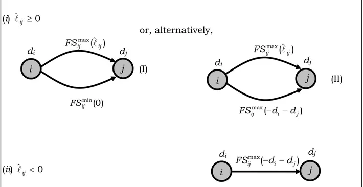
All the four GPRs with maximum time-lags correspond to the two finish-to-start scenarios depicted in Figure 2.
(i) ˆlij ≥0
(ii) ˆlij <0
Figure 2: Standardized representation of a resource incompatibility constraint combined with a maximum time-lag in terms of finish-to-start relations This representation on an AON network can be transformed in a network representation with zero time-lags, as depicted in Figure 3.
(i) ˆ ≥lij 0
(ii) ˆ <lij 0
Figure 3: Representation of a resource incompatibility constraint combined with a maximum time-lag in the transformed acyclic network
i i' di dj j i j dj di (II) ) ( max j i ij d d FS − − ) ˆ ( max ij ij FS l i j dj di ) ( max j i ij d d FS − − i j dj di ) ˆ ( max ij ij FS l ) 0 ( min ij FS (I) or, alternatively,
i
j
di' ≤ lˆijd
id
i'
di'' ≥ 0i''
i j di' ≤ lˆij di dj i' or, alternatively, di'' ≤ - (di + dj)i''
di' ≤ - (di + dj)In the latter picture, the dashed nodes are dummy nodes and the relations between any pair of adjacent nodes is of the type finish-to-start with zero time-lag. The durations associated with the dummy nodes are known only in terms of upper bounds and lower bounds.
2.2. A mathematical programming formulation
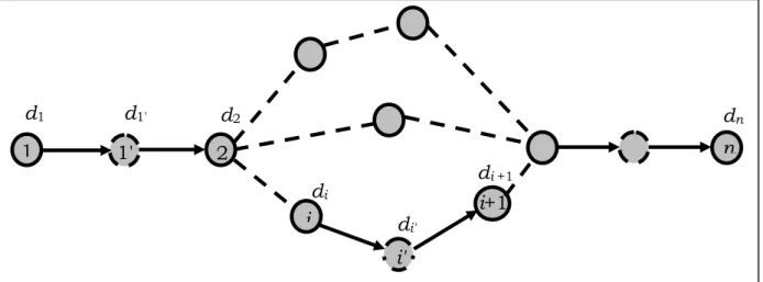
Following what we presented in the previous section, given a project with GPRs and resource incompatibility constraints only between pairs of activities with GPRs, we can use the AON network representation, shown in Figure 4, where only temporal constraints of the finish-to-start type with zero time-lags are present. 1 2 n i 1' d1' d1 d2 di dn i' di' i+1 di +1
Figure 4: A generic transformed AON acyclic network of the relaxed RCPSP-GPR.
The minimum sn is the optimal solution of the relaxed RCPSP-GPR, and then a
lower bound of the original problem. Let us now denote: • V the set of the nodes of the original network;
• V =Vg ∪VG ∪Vm ∪VM the set of dummy nodes of the transformed
network;
• V the subset of dummy nodes derived from the GPRs with minimum g
time-lags among pairs of activities for which no resource incompatibility exist;
• VG the subset of dummy nodes derived from the GPRs with maximum
time-lags among pairs of activities for which no resource incompatibility exist;
• Vmthe subset of dummy nodes derived from the GPRs with minimum
time-lags among pairs of activities for which resource incompatibility exist;
• VM =VM′ ∪VM′′ the subset of dummy nodes derived from the GPRs with
maximum time-lags among pairs of activities for which resource incompatibility exist;
• V ′ the subset of M VM such that ˆ ≥lij 0;
• V ′′ the subset of M VM such that ˆ <lij 0.
Moreover, V′M =VM′1 ∪VM′2 where
1
M
V ′ is the subset of dummy nodes
representing only the maximum time-lag constraints and V ′M2 is the subset of
dummy nodes representing only the resource incompatibility constraints compatible with the GPRs with maximum time lags (see Figure 3). Of course
2
1 M
M V
V′ = ′ .
Defining a binary variable to model the disjunctive scenarios defined in the
previous section, the problem of finding the minimum s
i
w′
n is that of computing
the minimum time to reach node n on that network and can be formulated in terms of mixed integer programming as follows.
min sn V P i V i d s si′ = i + i,∀ ′∈ , ∈ i′ ⊆ (1) V P i V i d s si = i′+ i′,∀ ∈ , ′∈ i ⊆ (2) g ij i m i i i i V i V d′ ≥ l′,l′ =δ′,∀ ′∈ ,l ′ =ˆl ∀ ′∈ (3) G M ij i i i i V V d′ ≤ l′,l ′ =ˆl ,∀ ′∈ ′1 ∪ (4) ' 2 , 0 , i M i i i Lw i V d′ ≥ − ′ +l′ l′ = ∀ ′∈ (5) 2 ), ( , ) 1 ( i i i i j M i L w d d i V d′ ≤ − ′ +l′ l′ = − + ∀ ′∈ ′ (6) " ' ), ( , ' ' ' i i i j M i d d i V d ≤ l l =− + ∀ ∈ (7)
{ }
0,1, i V w ∈ ∀ ′∈ ′ (8)V i R si ∈ + ∀ ′∈ ′ , (9)
{ }
1 \ , i V R si ∈ + ∀ ∈ (10) 0 1 = s (11)Constraints (1) and (2) model the finish-to-start relations in the acyclic network. Constraints (3), (4), (5), (6) and (7) model the bound on the values of
found from the analysis in the previous section. In particular, note that constraints (5) and (6) refer to the disjunctive situations depicted in Figures 2 and 3. In these constraints L is a very large positive number such that if
i d′ 1 = ′ i w constraints (5) are trivially satisfied and constraints (6) are effective; if wi′ =0 we have the opposite situation, i.e., constraints (5) are effective and constraints (6) are always satisfied. Constraints (8), (9), (10) and (11) define the range of variability of the decision variables.
Let us consider the linear relaxation of the above formulation, i.e., replacing constraint (8) with 2 , 1 M i i V w′ ≤ ∀ ′∈ ′ (8a) 2 , 0 M i i V w′ ≥ ∀ ′∈ ′ (8b)
and let us define the corresponding dual problem. To this end let us define the following dual variables yii',yi'i zi' zia' zib' w corresponding to constraints (1), i' (2), ((3),(4) and (7)), (5), (6), ((8a) and (8b)), respectively. The dual formulation of the previous relaxed problem is the following:
(14) , 1 (13) } , 1 { \ , 0 (12) ' , 0 ) ( max ' ' ' ' ' ' _ ' ' ' ' ' ' ' ' ' 2 ' ' 2 ' ' '' ' 1 ' ' ' ' ≤ ∈ ∀ ≤ − ∈ ∀ ≤ − ⎪⎭ ⎪ ⎬ ⎫ ⎪⎩ ⎪ ⎨ ⎧ + + + − + + +
∑
∑
∑
∑
∑
∑
∑
∑
∑ ∑
∑
∈ ∈ ∈ ∈ ∈ ∈ ′ ∈ ∪ ∪ ∈ ∈ ∈ ∈ ∪ n i i i i M M G M M i m g P i in S i ii P i i i S i i i P i ii V i i V i b i j i i V V V i i V i i S i V V i i ii i y n V i y y V i y y w z d d L z z y d l l) 24 ( ' , 0 ) 23 ( ' , 0 ) 22 ( ' , 0 ) 21 ( ' , 0 ) 20 ( ' , 0 ) 19 ( , ' free, ) 18 ( ' , free, (17) ' , 0 (16) ' , 0 (15) ' , 0 ' ' ' ' ' ' '' ' ' ' ' ' ' ' ' ' ' ' ' ' ' '' ' ' ' 2 2 2 1 2 2 1 M b i M a i M i G M M i g m i i i i i ii M i a i b i M b i a i i i G g M M m i i i V i z V i z V i w V V V i z V V i z S i V i y S i V i y V i w Lz Lz V i z z y V V V V V i z y ∈ ∀ ≥ ∈ ∀ ≥ ∈ ∀ ≤ ∪ ∪ ∈ ∀ ≤ ∪ ∈ ∀ ≥ ∈ ∈ ∀ ∈ ∈ ∀ ∈ ∀ ≤ + + − ∈ ∀ = − + − ∪ ∪ ∪ ∪ ∈ ∀ = + −
2.3. Analysis on the primal-dual formulation: main result
In this section, we provide the main result on the possibility to find the optimal solution to the problem in polynomial time O(m).
Exploiting the equality constraints (15) and (16) by substituting (15) in the objective function and (16) in constraint (17), we have the following equivalent mathematical formulation: ) 13 ( } , 1 { \ , 0 ) 12 ( ' , 0 ) ( max ' ' ' ' _ ' ' ' ' ' ' ' 2 ' ' 2 ' ' ' ' '' 1 ' ' n V i y y V i y y w z d d L y y d i i i i M M i i m M M g G S i ii P i i i S i i i P i ii V i i V i b i j i V i i S i S i V V V V V i i i ii i ∈ ∀ ≤ − ∈ ∀ ≤ − ⎪⎭ ⎪ ⎬ ⎫ ⎪⎩ ⎪ ⎨ ⎧ + + + − + +
∑
∑
∑
∑
∑
∑
∑ ∑
∑
∑
∈ ∈ ∈ ∈ ∈ ′ ∈ ∈ ∈ ∈ ′ ∈ ∪ ∪ ∪ ∪ l) 17 ( , ' , 0 ) 14 ( , 1 ' ' ' ' ' 2 i S a V i w Ly y i M i i i P i n in ′ ∈ ∈ ∈ ∀ ≤ + ≤
∑
) 24 ( ' , 0 ) 22 ( ' , 0 ) 19 ( , ' free, ) 19 ( , ' , 0 ) 19 ( , ' , 0 ) 18 ( ' , free, ' ' ' ' ' ' ' ' '' ' ' ' ' ' 2 2 2 1 M b i M i i M i i i G M M i i i g m i i i ii V i z V i w c S i V i y b S i V V V i y a S i V V i y S i V i y ∈ ∀ ≥ ∈ ∀ ≤ ∈ ∈ ∀ ∈ ∪ ∪ ∈ ∀ ≤ ∈ ∪ ∈ ∀ ≥ ∈ ∈ ∀Since L is positive and arbitrarily large and , the objective function is
maximized imposing that , where is the optimal value of .
Moreover, for the complementary slackness conditions referred to constraint (17a) we have that:
0 ' ≥ b i z 0 * = b z zb * zb ' i i' i ' ) ( ' , 0 ) ( * * ' * ' Ly' w' i V 2 i wi − ii − i = ∀ ∈ M
For node i’ we can have either or . Let us examine these two
situations separately. 0 * ' = i w * 1 ' = i w Case a: * 1. ' = i w
By (i) we have that
) ( ' , ' * * 2 ' ' Ly i V ii wi = − ii ∀ ∈ M By constraint (22) we have that:
) ( ' , 0 ' * 2 ' i V iii y M i i ≥ ∀ ∈
) 19 ( , ' , 0 ) 19 ( , ' , 0 ) 18 ( ' , free, ) 14 ( , 1 ) 13 ( } , 1 { \ , 0 ) 12 ( ' , 0 ' , where max ' '' ' ' ' ' ' ' ' ' ' ' ' ' _ ' ' ' ' ' ' ' 1 2 ' ' 2 ' ' ' b S i V V V i y d S i V V V i y S i V i y y n V i y y V i y y V i L y y d i G M M i i i g M m i i i ii P i n i S i ii P i i i S i ii P i ii M i V i i S i Vi S i i i ii i n i i i i i i ∈ ∪ ∪ ∈ ∀ ≤ ∈ ∪ ∪ ∈ ∀ ≥ ∈ ∈ ∀ ≤ ∈ ∀ ≤ − ∈ ∀ ≤ − ∈ ∀ − = ⎪⎭ ⎪ ⎬ ⎫ ⎪⎩ ⎪ ⎨ ⎧ +
∑
∑
∑
∑
∑
∑ ∑
∑ ∑
∈ ∈ ∈ ∈ ∈ ∈ ∈ ∈ ∈ l l Case b: * 0. ' = i wBy the complementary slackness property on constraint (8a) we have that
' * ' * 2 '(1 wi) 0, i' VM wi − = ∀ ∈
by which we obtain that
' *
' 0, ' M2
i i V
w = ∀ ∈ This implies that, by constraint (17),
' ' '* *, ' M2 b i a i z i V z ≤ ∀ ∈
Since the objective function is maximized imposing , we have that also
(see constraint (23)) 0 * ' = b i z ' '* 0, ' M2 a i i V z = ∀ ∈
) 21 ( ' , 0 ) 20 ( ' , 0 ) 19 ( , ' free, ) 18 ( ' , free, ) 16 ( ' , 0 ) 15 ( ' , 0 ) 14 ( , 1 ) 13 ( } , 1 { \ , 0 ) 12 ( ' , 0 max '' ' ' ' ' ' ' ' ' '' ' ' ' ' ' ' ' ' ' _ ' ' ' ' ' ' 1 2 1 ' ' '' ' 1 ' ' ' ' G M M i g m i i i i i ii M i i G g M M m i i i P i in S i ii P i i i S i i i P i ii V V V i i i V i i S i V V i i ii i V V V i z V V i z S i V i y S i V i y a V i y V V V V V i z y y n V i y y V i y y z z y d n i i i i G M M i m g ∪ ∪ ∈ ∀ ≤ ∪ ∈ ∀ ≥ ∈ ∈ ∀ ∈ ∈ ∀ ∈ ∀ = − ∪ ∪ ∪ ∪ ∈ ∀ = + − ≤ ∈ ∀ ≤ − ∈ ∀ ≤ − ⎪⎭ ⎪ ⎬ ⎫ ⎪⎩ ⎪ ⎨ ⎧ + +
∑
∑
∑
∑
∑
∑
∑ ∑
∑
∈ ∈ ∈ ∈ ∈ ∪ ∪ ∪ ∈ ∈ ∈ ∈ ∪ l lSubstituting now constraints (15) in the objective function we have the following formulation ) 13 ( } , 1 { \ , 0 ) 12 ( ' , 0 (16a) by ' 0 being ' , assign can we where max ' ' ' ' _ ' ' ' ' ' ' ' ' ' ' ' 2 2 ' ' ' n V i y y V i y y V i y V i L y y d i i i i i i S i ii P i i i S i i i P i ii M i i M i V i i S i Vi S i i i ii i ∈ ∀ ≤ − ∈ ∀ ≤ − ∈ ∀ = ∈ ∀ − = ⎪⎭ ⎪ ⎬ ⎫ ⎪⎩ ⎪ ⎨ ⎧ +
∑
∑
∑
∑
∑ ∑
∑ ∑
∈ ∈ ∈ ∈ ∈ ∈ ∈ ∈ l l) 19 ( , ' , 0 ) 19 ( , ' , 0 ) 18 ( ' , free, ) 16 ( ' , 0 ) 14 ( , 1 ' '' ' ' ' ' ' ' ' ' ' 1 2 b S i V V V i y d S i V V i y S i V i y a V i y y i G M M i i i g m i i i ii M ii P i n i n ∈ ∪ ∪ ∈ ∀ ≤ ∈ ∪ ∈ ∀ ≥ ∈ ∈ ∀ ∈ ∀ = ≤
∑
∈We note that in both the two cases analyzed we achieved the same
mathematical formulation, meaning that either w or w we can use
the same solution strategy. Moreover, we note that this mathematical model obtained is polynomially solvable in O(m) by means of a dynamic programming approach since the formulation has at most two variable per constraint (see Hochbaum and Naor, 1994). Furthermore, this formulation is the same as that found in absence of resource constraints by Bianco and Caramia, 2007. Therefore, there holds the property demonstrated in that paper, i.e., the optimal solution to our relaxed RCPSP-GPR, and therefore the lower bound of the original problem, is an augmenting path of maximum length on the described AON network where unit capacities have been installed on arcs.
0
* = * =1 '
i i'
3. Computational results
In this section, we show the results of our experimentation. Our algorithm and the other lower-bound algorithms used for comparison have been implemented in the C language. The machine used for the experiments is a Pentium IV PC with a 3GHz processor and 2Gb RAM. All the computing time are negligible (i.e., less than 1 seconds) and therefore are omitted in the presentation of the results.
In order to assess the quality of our lower bound with respect to state-of-the-art lower-bound algorithms, we have experimented the proposed approach on networks with 100 and 500 activities. These networks have been generated at random with the following parameters:
- Maximum number of initial (without predecessors) activities 10;
- Maximum number of terminal (without successors) activities 10;
- Maximum indegree of activities 5;
- Maximum time lag constraints ranging from 0% to 20% of the total
number of arcs;
We generated 90 problems for each network size, as done also in the RCPSP-max library, and reported our results in Figure 5 and Figure 6.
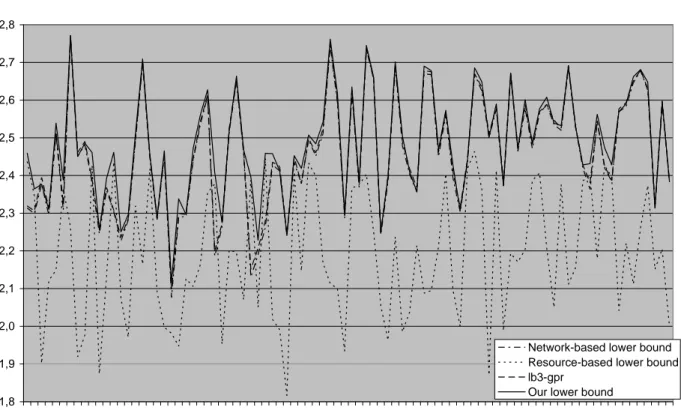
The chart in Figure 5 shows the performance of our lower bound, denoted in the following with Our_LB, compared to the network based lower bound, denoted with LB1, the resource-based lower bound, denoted with LB2, and the
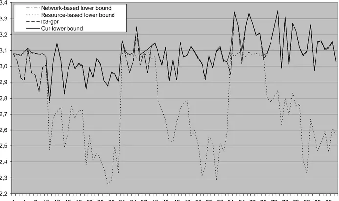
lb3-gpr lower bound, denoted with LB3, on 100 activity networks. Figure 6
reports the same comparison on 500 activity networks. Values in the y-axis are reported as base 10 logarithms.
Analyzing in detail the behaviour of LB1, LB2, and LB3, we notice that, as one can expect, LB2 is quite sensitive to the resource strength factor. Indeed, looking for instance at the chart in Figure 6 (where this appears clearer), we observe that for instances ranging from 1 to 10, from 31 to 40, and from 61 to 70, where the resource strength parameter is zero, LB2 outperforms LB1 and
LB3. For the other instance classes, whose resource strength parameter ranges
from 0.25 to 0.5, we have that the values of LB1 and LB3 tend to overlap (with LB3 having a slightly better behaviour) and dominate LB2.
Indeed, from a general viewpoint, while it appears that LB1 and LB3 tend to outperform LB2 on projects with 100 activities, it happens that there is not a striking dominance among LB1, LB2, and LB3 when 500 activities are considered.
Analysing the behaviour of Our_LB, one can note that it is robust to the different input instances, unlike the three competing lower bounds. In fact,
Our_LB is able to outperform LB1, LB2, and LB3 on all the tested instances. In
particular, by analysing the computational results, we note that, on 100 activity networks, Our_LB improves the best value among LB1, LB2, and LB3 by 5.2%, while on projects with 500 activities the improvement is 4.4%.
Moreover, considering the gaps (Our_LB-LBi/Our_LB), with i = 1,2,3, we have that Our_LB outperforms:
- LB1 by 9.2% for projects with 100 activities and by 22.6 for projects with 500 activities,
- LB2 by 38.4% and by 65.2% in the scenarios with 100 and 500 activities, respectively,
- LB3 by 8.9% on instances with 100 activities and by 21.4% on 500 activities. 1,8 1,9 2,0 2,1 2,2 2,3 2,4 2,5 2,6 2,7 2,8 1 4 7 10 13 16 19 22 25 28 31 34 37 40 43 46 49 52 55 58 61 64 67 70 73 76 79 82 85 88 Network-based lower bound Resource-based lower bound lb3-gpr
Our lower bound
Figure 5: Comparison among our lower bound, the resource-based lower
2,2 2,3 2,4 2,5 2,6 2,7 2,8 2,9 3,0 3,1 3,2 3,3 3,4 1 4 7 10 13 16 19 22 25 28 31 34 37 40 43 46 49 52 55 58 61 64 67 70 73 76 79 82 85 88 Network-based lower bound
Resource-based lower bound lb3-gpr
Our lower bound
Figure 6: Comparison among our lower bound, the resource-based lower
bound, the network-based one, and lb3-gpr (500 activity networks).
Conclusions
In this paper we studied a new lower bound on the resource-constrained project scheduling problem with generalized precedence relationships. This lower bound is based on a mathematical formulation of a relaxation of the original problem, where only precedence relationships between pairs of activities associated with GPRs are considered. We showed that the proposed lower bound behaves satisfactorily on project networks with different sizes when compared to known lower bounds from the state of the art.
Acknowledgements
The authors are grateful to two anonymous referees for their suggestions and comments that improved the paper.
References
Bartusch, M., R.H. Mohring and F.J. Radermacher (1988). Scheduling Project Networks with Resource Constraints and Time Windows. Annals of Operations Research, 16, 201-240.
Bianco, L. and M. Caramia (2007). A New Formulation of the Resource-Unconstrained Project Scheduling Problem with Generalized Precedence Relations to Minimize the Completion Time. Technical Report DII - University of Rome “Tor Vergata”, submitted (downloadable from http://www.dii.uniroma2.it/doc/gprs.pdf).
Bianco, L. and M. Caramia (2008). A New Approach for the Project Scheduling
Problem with Generalized Precedence Relations. Proceedings of the 11th
International Workshop on Project Management and Scheduling, Istanbul, April 28-30, 2008.
Blazewicz, J., J.K. Lenstra and A.H.G. Rinnooy Kan (1983). Scheduling subject to resource constraints: Classification and complexity. Discrete Applied Mathematics 5 (1), 11–24.
Demeulemeester, E.L. and W.S. Herroelen (1997a). New benchmark results for the resource-constrained project scheduling problem. Management Science 43 (11), 1485-1492.
Demeulemeester, E.L. and W.S. Herroelen (1997b). A branch-and-bound procedure for the generalized resource-constrained project scheduling problem. Operations Research 45, 201-212.
Demeulemeester, E.L. and W.S. Herroelen (2002). Project Scheduling - A Research Handbook. Kluwer Academic Publishers, Boston.
De Reyck, B. (1998). Scheduling Projects with Generalized Precedence Relations - Exact and Heuristic Approaches. Ph.D. Thesis, Department of Applied Economics. Katholieke Universiteit Leuven, Leuven, Belgium.
De Reyck, B. and W. Herroelen (1998). A branch-and-bound procedure for the resource-constrained project scheduling problem with generalized precedence relations. European Journal of Operational Research, 111 (1), 152-174.
Dorndorf, U. (2002). Project Scheduling with Time Windows. Physica-Verlag. Elmaghraby, S.E.E. and J. Kamburowski (1992). The Analysis of Activity
Networks under Generalized Precedence Relations (GPRs). Management Science 38 (9), 1245-1263.
Hochbaum, D., J. Naor (1994). Simple and Fast Algorithms for Linear and Integer Programs with Two Variables per Inequality. SIAM Journal on Computing 23(6) 1179-1192.
Klein, R. and A. Scholl, (1999). Computing lower bounds by destructive improvement: An application to resource-constrained project scheduling. European Journal of Operational Research 112, 322-346.
Neumann, K., C. Schwindt and J. Zimmerman (2002). Project Scheduling with Time Windows and Scarce Resources. Lecture Notes in Economics and Mathematical Systems 508, Springer, Berlin.