Investigating the conclusive phases of galaxy evolution: from star formation to quiescence

(1)

Alma Mater Studiorum – Università di Bologna

DOTTORATO DI RICERCA IN

ASTROFISICA

ciclo XXX

Settore Concorsuale: 02/C1

Settore Scientifico Disciplinare: FIS/05

Investigating the conclusive phases of galaxy evolution:

from star formation to quiescence

Presentata da: Annalisa Citro

Coordinatore Dottorato

Relatore

Prof. Francesco Rosario Ferraro

Prof. Andrea Cimatti

Correlatori:

Dott.ssa Lucia Pozzetti

(2)

——————————————————————————————————————-Nonostante i progressi fatti verso una più profonda comprensione dell’evoluzione delle galassie, manca ancora una visione completa di quali siano i meccanismi che re-golano la formazione sellare nelle galassie, di come le proprietaà evolutive delle galassie correlino con le loro masse e tassi di formazione stellare e quali processi siano respons-abili dello spegnimento della formazione stellare e i loro tempi-scala.

In questo lavoro di tesi, si è cercato di rispondere ad alcune di queste domande aperte, studiando l’evoluzione delle galassie a ritroso nel tempo. In particolare, siamo partiti dallo studio archeologico di galassie passive locali (1), ricostruendo le loro storie di for-mazione stellare. Abbiamo poi fatto un passo indietro verso la fase in cui le galassie spengono la loro formazione stellare (2), definendo una nuova metodologia che ci per-metta di identificare i progenitori delle galassie passive nella fase immediatamente suc-cessiva all’interruzione della formazione stellare. Infine, siamo andati ancora più in-dietro nel tempo, studiando la fase in cui le galassie formano stelle (3), analizzando le proprietà di galassie ad alto redshift che potrebbero essere i progenitori delle galassie passive locali.

I nostri studi si sono basati sull’analisi spettrale delle galassie. In particolare, abbiamo studiato la fase passiva e quella star-forming sfruttando l’informazione contenuta nella totalità degli spettri delle galassie analizzate, la cui forma dipende dalle caratteristiche delle popolazioni stellari. La fase di spegnimento della formazione stellare è stata in-vece analizzata usando rapporti tra righe di emissione, che sono collegate al mezzo interstellare e al suo stato di ionizzazione durante o subito dopo lo spegnimento della formazione stellare.

I nostri più importanti risultati possono essere riassunti come segue:

1. Riguardo le galassie passive locali, abbiamo analizzato gli spettri stacked mediani di ⇠ 25000 galassie early-type (ETGs) passive e massive (log(M/MJ₎ _{& 10}10.75₎

osservate dalla Sloan Digital Sky Survey (SDSS) DR4 a redshift z < 0.3, usando la tecnica del full-spectrum fitting (STARLIGHT, Cid Fernandes et al., 2005). Ab-biamo trovato che questo methodo è in grado di recuperare le proprietà evo-lutive delle galassie (i.e. età, metallicità, estinzione da polvere) e le loro storie di formazione stellare con una accuratezza maggiore del 10% a partire da rap-porti segnale-rumore& 10 20. Abbiamo trovato evidenze di evoluzione down-sizing (Cowie et al., 1996), sia nelle età che nelle storie di formazione stellare. Queste ultime hanno la forma: SFR(t) / ⌧ (c+1)_{t c exp( t/⌧ )}_{e sono più brevi per}

galassie più massive. Dalle storie di formazione stellare che abbiamo ricostruito, abbiamo dedotto le proprietà dei progenitori delle galassie early-type analizzate, trovando che questi debbano aver avuto un alto tasso di formazione stellare (i.e. ⇠ 350 400 MJ_yr 1_{) ed alte masse a redshift z ⇠ 4 5, diventando quiescenti a}

partire da z ⇠ 1.5 2.

Questi risultati sono descritti in Citro et al. 2016; Astronomy & Astrophysics, Volume 592, id.A19, 22 pp.

2. Riguardo la fase di spegnimento della formazione stellare, abbiamo proposto una nuova metodologia capace di identificare le galassie star-forming nella fasi imme-diatamente successive all’interruzione della formazione stellare. Questa

(3)

metodolo-gia è basata sull’utilizzo di rapporti tra righe di emissione di alta e bassa ioniz-zazione. In particolare, ci siamo focalizzati sui due rapporti [O III] 5007/H↵ e [Ne III] 3869/[O II] 3727, che sono stati modellati con il codice di fotoion-izzazione CLOUDY (Ferland et al.,1998,Ferland et al.,2013). Abbiamo trovato che essi sono ottimi traccianti delle fasi immediatamente successive allo spegni-mento della formazione stellare, dato che diminuiscono di un fattore ⇠ 2 in circa ⇠ 80 – 90 Myr dal momento della sua interruzione. Abbiamo mitigato la degener-azione tra lo stato di ionizzdegener-azione/età e la metallicitià che compromette il nostro approccio introducendo il nuovo diagramma diagnostico [O III] 5007/H↵ vs. [N II] 6584/[O II] 3727. Usando un campione di galassie star-forming selezionate dalla SDSS DR8, abbiamo identificato in questo piano 10 esempi di galassie che stanno spegnendo la loro formazione stellare (i.e. le più estreme), che potrebbero essere i progenitori in fase di spegnimento delle galassie passive studiate prece-dentemente (che erano passive a z . 2). Abbiamo trovato che queste 10 galassie sono caratterizzate da continui blu e da colori (u r)più blu di quelli tipici della Green Valley, come ci si aspetta se la formazione stellare in esse si è spenta nel passato molto recente.

Questi risultati sono descritti in Citro et al. 2017; Monthly Notices of the Royal Astro-nomical Society, Volume 469, Issue 3, p.3108-3124.

3. Riguardo la fase star-forming ad alto redshift, abbiamo analizzato gli spettri stacked mediani ultravioletti di 290 galassie star-forming a 2  z  4. In particolare, ci siamo focalizzati sul campione ad oggi disponibile della survey spettroscopica ESO-VLT VANDELS (PIs: Ross McLure, Laura Pentericci), della quale faccio at-tualmente parte. Il nostro scopo principale è stato quello di usare il metodo del full-spectrum fitting per derivare le proprietà evolutive di tali galassie, connet-tendole allo studio archeologico delle ETGs condotto precedentemente. Abbiamo trovato che, se le righe di assorbimento spettrali che includono anche un contrib-uto di assorbimento dal mezzo interstellare (che non sono modellate dagli attuali modelli di sintesi di popolazioni stellari) vengono escluse dal fit, risultati affidabili sono ancora ottenuti a partire da rapporti segnale-rumore ⇠ 10 – 20, ma con una accuratezza minore rispetto al caso in cui solo le forti righe di emissione vengono escluse dal fit. Dall’analisi spettrale delle galassie VANDELS abbiamo dedotto età più vecchie ed estinzione da polvere più alta per le galassie più massive, mentre non sono emersi andamenti significativi della metallicità in funzione della massa. Inoltre, le storie di formazione stellare sembrano essere più prolungate ad alte masse. Tutti questi risultati saranno confermati da analisi ulteriori condotte sul campione totale di galassie star-forming VANDELS, che ammonterà a ⇠ 800 spet-tri.

(4)

——————————————————————————————————————-Despite the progress made towards a more comprehensive knowledge of galaxy evo-lution, a global picture of the mechanisms regulating the formation of stars in galaxies, of how galaxy evolutionary properties correlate with stellar masses and star formation rates (SFRs) and of the processes suppressing the star formation in galaxies and their timescales is still lacking.

In this thesis work, we attempt to address some of these open questions, inspecting galaxy evolution back in cosmic time. In particular, we start from the archaeological analysis of passive local galaxies (1), reconstructing their past star formation histories. Then we take a step back towards the phase in which galaxies quench their star for-mation (2), defining a new methodology able to identify the quenching progenitors of passive galaxies. Finally, we move back to the star-forming phase (3), investigating the properties of high-redshift galaxies which could be the star-forming progenitors of the passive local ones.

Our investigations mainly rely on the spectral analysis of galaxies. In particular, we study both the passive and star-forming phase by exploiting the information contained in the galaxy full-spectrum, whose shape depends on the properties of the underlying stellar populations. The quenching phase is instead investigated by means of emission line ratios, which are associated to the Interstellar Medium (ISM) and its ionization state during or just after the star formation has stopped.

The main results obtained from our backward reconstruction of galaxy evolution can be summarized as follows:

1. Concerning passive local galaxies, we analyze the median stacked spectra of ⇠ 25000 massive (log(M/MJ_{& 10}10.75_{) and passive Sloan Digital Sky Survey (SDSS)}

DR4 early-type galaxies (ETGs) at z < 0.3 by means of the full-spectrum fitting (STARLIGHT,Cid Fernandes et al.,2005). We find that this method is able to re-trieve the evolutionary properties (i.e. ages, metallicities, dust extinctions) and the SFHs with an accuracy higher than 10% starting from signal-to-noise ratios (SNRs)& 10 20. We find evidence of a downsizing evolution (Cowie et al.,1996), both in ages and SFHs. The latter are of the form SFR(t) / ⌧ (c+1)_{t c exp( t/⌧ )}

and are shorter for more massive galaxies than for less massive ones. From the reconstructed SFHs, we place constraints on the properties of the progenitors of the studied ETGs, arguing that they should have been vigorously star-forming – with star formation rates (SFRs) ⇠ 350 400 MJ_yr 1_{– at z ⇠ 4 5, and quiescent}

by z ⇠ 1.5 2.

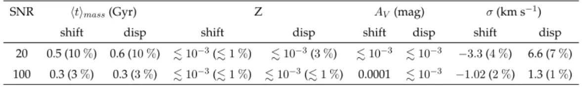
These results can be found in Citro et al. 2016; Astronomy & Astrophysics, Volume 592, id.A19, 22 pp.

2. Concerning the quenching phase of galaxies, we propose a new methodology aimed at finding star-forming galaxies which just quenched their star-formation, based on emission line ratios involving high- and low-ionization potential lines. We focused on the [O III] 5007/H↵ and [Ne III] 3869/[O II] 3727 emission line ratios, which are modelled with the CLOUDY photoionization code (Ferland et al.,1998, Ferland et al.,2013). We find that they are very good tracers of the early epochs of quenching, dropping by a factor ⇠ 2 in ⇠ 80 – 90 Myr from the

(5)

time of the quenching. We mitigate the ionization/age-metallicity degeneracy af-fecting the proposed methodology by introducing the [O III] 5007/H↵ vs. [N II] 6584/[O II] 3727 diagnostic diagram. Using a sample of SDSS DR8 star-forming galaxies, we identify 10 examples of quenching candidates within this plane (i.e. the most extreme ones), which could be the low redshift, quenching progenitors of the ETGs studied earlier on (which are quiescent by z ⇠ 1.5 2). We find that the 10 galaxies are characterized by blue dust-corrected continua and by (u r) colours bluer than the Green Valley ones, as expected if the star formation quench-ing has occurred in the very recent past.

These results can be found in Citro et al. 2017; Monthly Notices of the Royal Astronomical Society, Volume 469, Issue 3, p.3108-3124.

3. Concerning the star-forming high-redshift phase, we analyzed 6 UV median stacked spectra obtained from a sample of star-forming galaxies at high redshift. In par-ticular, we studied the 290 star-forming and Lyman break galaxies so far available from the on-going ESO-VLT public spectroscopic survey VANDELS (PIs: Ross McLure, Laura Pentericci), where I am involved. These galaxies have 2  z  4 and 8 < log(M/MJ_{) < 11.5. Our main aim is to derive the evolutionary}

proper-ties (i.e. ages, metalliciproper-ties, dust extinctions) and the SFHs of these galaxies by means of the full-spectrum fitting, connecting them to our archaeological study of ETGs. We find that if absorption lines including ISM contributions (which are not modelled by the current evolutionary stellar population synthesis models) are ex-cluded from the spectral fit, reliable results are still retrieved from SNRs ⇠ 10 – 20, although with a slightly larger dispersion with respect to the case in which only the strongest emission lines are excluded from the fit. The spectral fit of VAN-DELS spectra provides older ages and larger dust extinctions for more massive galaxies than for less massive ones, while no clear metallicity trend is observed as a function of mass. The SFHs appear to be more prolonged at lower masses than at higher ones. All these results will be confirmed by further analyses performed on the total sample of VANDELS star-forming galaxies, which will amount to ⇠ 800 spectra.

(6)

List of Figures

1.1 Optical stacked spectrum of ⇠ 2800 SDSS ETGs with M ⇠ 1010.86_MJ

and median z ⇠ 0.11. Vertical lines mark some absorption features. Black lines are metallic absorptions (from left to right: MgI, NaD); green lines are Balmer absorptions (from left to right: H , H↵); the grey shaded band mark the location of the G Band; blue shaded bands mark the location of the D4000 continuum discontinuity (also known as the D4000 break). . . . 3

1.2 The (U V )– MV color-magnitude relation for galaxies that are spectro-scopic members of the Coma cluster (from Bower et al. 1999). . . 4

1.3 The infrared fundamental plane of elliptical galaxies (fromMagoulas et al.,

2012). . . 5

1.4 Sketch of the downsizing evolution scenario (fromThomas et al.,2010). Specific star formation rate as function of look-back time for early-type galaxies of various masses as indicated by the labels. It is clear that, for higher masses, the peak of the sSFR occurs earlier and the duration of the star formation is shorter. . . 9

1.5 Number density evolution of the sample galaxies in various mass bins. The dotted lines correspond to the no-evolution solution normalized at z= 0 (fromPozzetti et al.,2010). . . 11

1.6 The (u r)color-mass diagram as observed bySchawinski et al.(2014). The top left panel show the whole population of galaxies. The top and bottom right panels show the early-type and late-type galaxies, respec-tively. Green lines mark the green valley region. . . 12

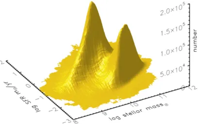
1.7 The 3D SFR-mass relation for local galaxies in the SDSS database and 0.02 < z < 0.085(FromRenzini & Peng,2015). . . 16 1.8 Fundametal metallicity relation (fromMannucci et al.,2010). Circles are

the median values of metallicity of local SDSS galaxies in bin of M and SFR, with SFR decreasing from blue to red. . . 18

2.1 STARLIGHT typical output. Top panel. Grey curve: input spectrum; blue curve: best fit model, red vertical line: normalization wavelength. Small panel shows the differences between the input and the best fit model spectrum in function of wavelength. Bottom panel. STARLIGHT light fractions xj’s. The x-axis contains the ages of all the library models, the

y-axis contains the light contribution (in percentage) to the best fit model at the normalization wavelength for each library model (in particular: green is for Z = 0.02 (solar metallicity), red and magenta stand for Z = 0.05 and Z = 0.008, respectively). . . 29

(9)

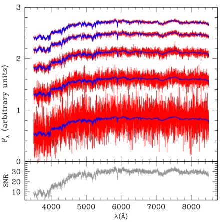
2.2 Simulated spectra of a CSP at 13 Gyr from the onset of the SFH (exponen-tially delayed with ⌧ = 0.3 Gyr), with solar metallicity and SNR 2, 5, 10, 20 and 30, increasing form bottom to top. For each SNR, the blue curve is the starting BC03 model used for the simulation, while the red curve is the the simulated spectrum. The lower panel shows the behaviour of the SNR as a function of wavelength for a simulated spectra with SNR = 30 in the 6500 – 7000 Å window. . . 30

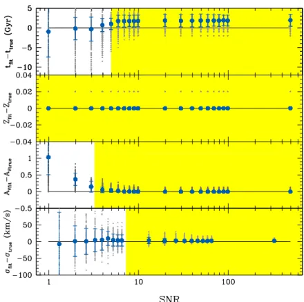
2.3 Retrieved ages, metallicities, dust extinctions and velocity dispersions as a function of the mean SNR of the input spectra. Blue filled circles are the differences, averaged on all the computed simulations (i.e. 10 ⇥ 13 models), between the ouptut and the input weighted ages, mass-weighted metallicities, dust extinctions and velocity dispersions (from top to bottom); blue vertical bars are the median absolute deviations (MAD) on all the computed simulations; grey points are the differences derived from each individual simulation; yellow shaded regions in each panel in-dicate the minimum SNR from which the accuracy of the input retrieving is better than 10 %. . . 34

2.4 Recovery of star formation histories. The four panels show a CSP at 3, 5, 7 and 11 Gyr from the onset of the SFH. Black vertical lines represent the exponentially delayed SFH (⌧ = 0.3 Gyr) assumed for the input spectra (rebinned according to the age step of our library models), while vertical lines represent the output SFH; horizontal arrows indicate the time from the beginning of the SF (i.e. 3, 5, 7 and 11 Gyr, respectively), while grey vertical lines mark the asymmetric age ranges around the SFH peak de-fined in the text for CSPs younger or older than 5 Gyr (i.e. [ 1; + 0.5] and [ 1.5; + 1], respectively).. . . 35

2.5 Recovery of star formation histories. The four panels show a CSP at 3, 5, 7, and 11 Gyr from the onset of the SFH. In the two top panels, red triangles indicate the median mass fractions retrieved within [ 1; + 0.5] Gyr from the SFH peak; in the two bottom panels, they are the median mass fractions within [ 1.5; + 1] Gyr (as described in the text). In all four panels, cyan circles are the median mass fractions relative to stellar populations younger than 0.5 Gyr, while red and cyan horizontal lines mark the expected mass fraction within the defined age ranges and below 0.5 Gyr, respectively. . . 36

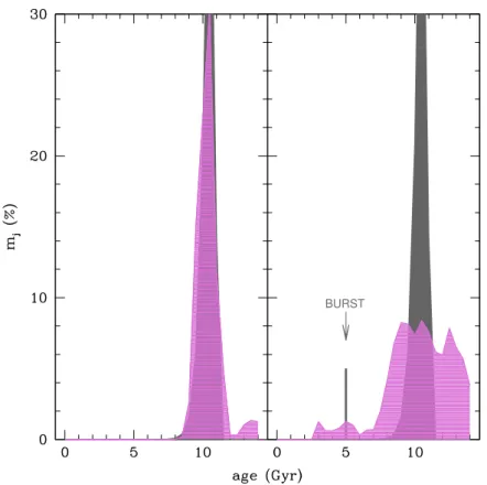
2.6 Retrieving of more complex SFH. Left panel: output SFH (pink curve) obtained when an input SFH (grey curve) including only a single CSP is considered; right panel: output SFH (pink curve) obtained when an input SFH (grey curve and vertical line) including a single CSP plus a later burst (which happens 6 Gyr after the main SF episode and contributes to the 5 %in mass) is considered. . . 38

(10)

curves) obtained when the input SFH (grey curves and vertical lines) in-cludes a single CSP plus a later burst happening 6 Gyr after the main SF episode and contributing in mass by 3, 5 and 10 % (from top to bottom). Right panels show the output SFH (pink curves) obtained when the in-put SFH (grey curves and vertical lines) includes a single CSP plus a later burst of SF contributing in mass by 5 %, and happening 4, 6, 8 Gyr after the main SF event (from top to bottom). . . 39

2.8 The same of Fig. 2.3, but using the MS11 spectral library to retrieve the evolutionary properties. . . 40

2.9 Mass-redshift relation of the adopted sample. Each grey point represents a galaxy; colored triangles and vertical bars represent the median masses and corresponding MADs of each mass and redshift bin (with mass in-creasing from yellow to violet). . . 42

2.10 SDSS median stacked spectra for the sample of massive and passive ETGs. Left and right upper panels show, respectively, median stacked spectra with a fixed redshift (0.15. z . 0.19) and different masses (with mass in-creasing from blue to red) and with a fixed mass (11.25 < log(M/MJ_{) <}

11.5) and four different redshifts (0.04, 0.08, 0.16, 0.23) (with redshift in-creasing from blue to red). Lower panels illustrate the fractional differ-ences (defined as (fi fREF/fREF)⇥ 100, where fiis the flux of the i-th

spectrum and fREF is the reference one) among the stacked spectra as a

function of wavelength. In particular, to show the redshift and the mass dependence we used as reference, respectively, the median stacked spec-trum obtained for 11.25 < log(M/MJ_{) < 11.5}_{and 0.07 < z < 0.09, and}

the one corresponding to 10.75 < log(M/MJ_{) < 11}_{and 0.15 < z < 0.17.}

Vertical grey lines mark some of the best-known absorption lines. . . 43

2.11 Typical output of the full-spectrum fitting procedure using BC03 (left) and MS11 (right) spectral synthesis models. In particular, we show the case of the median stacked spectrum derived for 11 < log(M/MJ_{) <}

11.25 and z ⇠ 0.05. In the top panel the black curve is the observed spectrum, the red curve is the best fit model and grey shaded regions are the masked spectral regions (see Table 2.3). In the bottom panel the ratio of the best fit model spectrum to the observed flux is shown. . . 44

2.12 Mass-weighted (top) and light-weighted (bottom) age-redshift relations (for BC03 models). Stellar mass increases from blue to red. The black line is the age of the Universe, while grey lines are the age of galaxies assuming different formation redshifts. . . 46

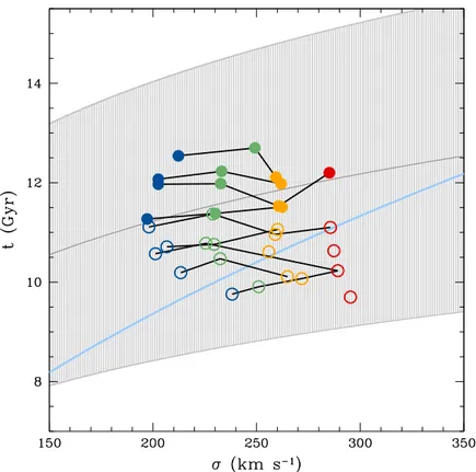
2.13 Mass-weighted ages as a function of the velocity dispersion for BC03 models (symbols are color-coded as in Fig. 2.12). Filled circles are the mass-weighted ages corresponding to z < 0.1, matching the redshifts analyzed byMcDermid et al.(2015), with black curves linking the mass-weighted ages related to different mass bins but similar redshifts. The grey curve is the age – relation inferred by McDermid et al. (2015) with its dispersion (grey shaded region), while the light-blue curve is the

Thomas et al.(2010) relation (its dispersion, not shown in the figure, is of the order of ⇠ 60 %). . . 47

(11)

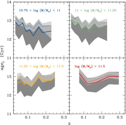
2.14 agef-redshift relations for the four mass bins. Solid and dotted curves

(color coded as in Fig. 2.12) are the ages of formation as a function of red-shift referring, respectively, to BC03 and MS11 spectral synthesis models. Dark-grey and light-grey shaded regions are the 1 dispersions calcu-lated starting from the 16th (P16) and 84th (P84) percentiles of the mass fraction cumulative function for BC03 and MS11 models, respectively. . . 48

2.15 Mass fractions mjas a function of look-back time for the four mass bins,

with mass increasing from top to bottom (in the case of BC03 models). Colored vertical lines (color-coded as in Fig. 2.12) are the mj obtained

from the full-spectrum fitting for each mass bin, put in phase according to their P50. In each mass bin, black vertical lines mark the P50 of the distribution, obtained from data as an average on the P50 of all the red-shift bins, while black horizontal lines are the median dispersions [P50 – P16] and [P84 – P50]. The corresponding asymmetric gaussians (grey) are overplotted to the mj distributions. On the top of the figure, the zF

corresponding to each agefare indicated. . . 49

2.16 Mass fractions mj recovered from the full-spectrum fitting as a function

of redshift in the case of BC03 models. Red and blue curves refer, respec-tively, to stellar populations older and younger than 5 Gyr, with darker colors standing for higher stellar masses. . . 50

2.17 SFHs derived from median stacked spectra. Mass increases from top to bottom, redshift increases from left to right, as indicated. Note that no significant episodes of SF occurred after the main SF event. The mass fractions relative to stellar population younger than 5 Gyr is very low (i.e.. 5 %).. . . 53

2.18 SFH for the four mass bins of our sample, with mass increasing from top to bottom (in the case of BC03 models). Colored vertical lines are the SFR (MJ_yr 1_{) derived from the m}

jprovided by the spectral fitting (colors are

coded as in Fig. 2.12). In each mass bin, black vertical and horizontal lines are defined as in Fig. 2.15. In each panel, we show the two best fit models deriving from the assumption of an Expdel (dotted curves) or an Expdelc (solid curves) parametric function to describe the derived SFHs. The best fit parameters are also reported. Pink curves are the inverted-⌧ models with ⌧ = 0.3 Gyr described in the text, extended up to 13.48 Gyr (which corresponds to the age of the Universe in the assumed cosmology). . . 54

2.19 Mass weighted metallicities as a function of mass and redshift. Solid and dotted curves refer to BC03 and MS11 models, respectively. Stellar mass increases from blue to red, as indicated in the top right of the figure. . . . 55

2.20 Comparison between our mass-weighted metallicities (in the case of BC03 models) and the values reported in the literature. In particular, colored filled circles (color-coded as in Fig. 2.12) are our results (the cyan curve is a second order fit to our data); the grey curve is the scaling relation pro-vided byThomas et al.(2010), with its dispersion (grey shaded region), while black open circles and vertical bars are the measures (and disper-sions) performed on our sample byGallazzi et al.(2005). The light-brown curve is the relation derived byMcDermid et al.(2015), together with its dispersion (light-brown shaded region). . . 56

(12)

bin (the values of are illustrated together with the errors MAD/pN), with the size of the triangles increasing for increasing redshift; black open circles are the velocity dispersions derived from the re-reduction of SDSS spectra performed by the Princeton Group, used for comparison. . . 57

2.22 Dust extinction AV as a function of redshift and mass. Solid and dotted

curves refer to BC03 and MS11 models, respectively. Colors are coded as in Fig. 2.12. . . 58

2.23 Comparison between the median ages, metallicities, velocity dispersions and dust extinction derived from median stacked spectra (open circles) and individual spectra (open triangles) in the case of BC03 models (verti-cal bars are the MADs on the results from individual spectra) for the two mass bins 11.25 < log(M/MJ_{) < 11.5}_{(left) and log(M/M}J_{) > 11.5}_(right). ₅₉

2.24 Evolving SFR – mass curves (in the case of BC03 models and for the Expdelcparametric form). The four dotted curves are the evolving SFR – mass relations for the four mass bins of our sample (deduced from the SFHs of Fig. 2.18) as a function of cosmic time (from left to right), color coded as in Fig. 2.18. Blue, black, green, red, cyan and magenta lines are the SFR – mass relations deduced by different authors at various red-shifts (as indicated in the top left of the figure), within their observed mass ranges (solid lines). Filled circles are the SFR for the four mass bins at various z, corresponding to the ones reported in the top left of the fig-ure (note that, at z ⇠ 0, we derive log(SF R) < 3, thus the values at this redshift are not included in the plot). The grey dashed-dotted line repre-sents the level of SFR at which the galaxies can be considered completely quiescent.. . . 62

2.25 Evolving sSFR – z relations for the Expdelc parametric form. Solid and dotted curves are the sSFR – z relations for the four mass bins (color coded as in Fig. 2.18) for BC03 and MS11 models, respectively. Blue, black, green, cyan and red open circles (and violet open triangle) are the sSFR estimates obtained by various authors at different redshifts (for the four mass bins), as indicated in the top left of the figure. The grey horizon-tal dashed-dotted line marks the level of sSFR at which a galaxy is in general considered completely quiescent (sSFR. 10 11_yr 1_{). Dark-grey}

and light-grey shaded regions represent the uncertainty on the look-back time, associated to the results from BC03 and MS11 models, respectively. . 63

2.26 Size – mass relation derived for our sample of massive, passive ETGs (red) and for the parent sample of local galaxies with log(M/MJ_{) > 10.75}

(grey) (Kauffmann et al.,2003stellar masses are rescaled to the M11 ones). Colored points represent the two samples; solid curves are the P50 of the Redistribution at each mass. The dashed red curves and the shaded grey

region includes the 68 % of the Re distribution of the passive and the

(13)

2.27 Number density above log(M/MJ_{) = 10.75. The central colored bands}

are the ⇢nof the ETG progenitors as a function of the look-back time in the

case of BC03 (upper panel) and MS11 (lower panel) models, derived from the SFHs of the analyzed ETGs, together with its uncertainty (± 0.1 dex) and the uncertainty on the look-back time (i.e. +0.6

1.1Gyr, considering the

small ⇠ 0.5 Gyr systematic introduced by median stacked spectra, see Sect. 2.6). The red and the blue parts cover, respectively, the redshift inter-val within which ETGs are completely quiescent or star-forming. At each cosmic epoch, the literature results are illustrated with red, blue and black symbols, which refer to the ⇢nof the quiescent, the star-forming and the

global galaxy population (i.e. star-forming + quiescent galaxies), respec-tively (all above the same mass threshold). In more detail, closed triangles and cirlces are theIlbert et al.(2013) and theMuzzin et al.(2013a) ⇢n,

re-spectively; open triangles and circles are theMancini et al.(2009) and the

Domínguez Sánchez et al.(2011) values, respectively; open square and star are theGrazian et al.(2015) and theCaputi et al.(2015) values, re-spectively. The shaded colored regions emphasize the uncertainties on the literature number densities (at each cosmic time, we consider the out-ermost envelope which includes all the literature estimates, taking into account their uncertainties). It is important to note that the literature ⇢n

and their associated errors are derived by integrating the GSMF inferred through the 1/Vmaxmethod, and by computing the quadrature sum of its

errors. TheMuzzin et al.(2013a) error estimates (obtained from the best fit Schechter functions) are also shown in grey. . . 66

3.1 Heating and cooling rates for two photoionized cells of gas. The solid curves show results for low-density (102_cm3_{) gas with abundances}

sim-ilar to the Orion Nebula. Grains exist and refractory elements have de-pleted abundances. The dashed curve shows a higher-density gas (108_cm3₎

with solar abundances and no grains. Both volume heating and cooling rates have been divided by the square of the density to bring out the ho-mology relations between the heating and cooling quantities (From Fer-land(2003)). . . 76

3.2 Sketch describing the effect of the star-formation quenching on high- and low-ionization potential lines. When the SF is halted, the most massive O stars die on timescales of 10 – 100 Myr. As a consequence, the high-ionization lines, which can be only produced by these stars, disappear from the galaxy spectrum. On the contrary, low-ionization lines, which need the softer photons provided by B stars to be produced, survive at longer times in the spectra (from Quai et al. 2017, submitted). . . 79

3.3 Time evolution of a Starburst99 SSP SED with solar metallicity (spectra get older from blue to orange, as reported in the top left of the figure). Black dotted vertical lines indicate the wavelengths corresponding to the ionization energies of the emission lines analysed in this Chapter, as indi-cated. . . 81

(14)

ionization potential (i.e. 13.6 eV) and thus are illustrated within the same panel. Curves are relative to a Starburst99 SSP with log(M/MJ_{) = 10}6

and three different metallicities (Z = 0.004, dashed; Z = 0.02, solid; Z = 0.04, dotted). . . 81

3.5 Comparison between our models and observations. Dark grey points are galaxies extracted from the SDSS DR8 with S/N(H↵) > 5, S/N(H ) > 3 and S/N([N II]), S/N([O III]) > 2, while light grey points are galaxies with S/N([O III])< 2. The superimposed grid is our set of fixed-age models with different metallicities (Z = 0.004 blue; Z = 0.008 cyan; Z = 0.02 green; Z = 0.04 red) and different log(U)0 (going from 3.6 to 2.5 with steps

of 0.1 dex from bottom to top). Black curves mark the levels log(U)0 =

3.6, 3, 2.5, from bottom to top, as indicated. . . 84

3.6 Comparison among our models (solid curves),Levesque et al.(2010) (dashed curves) andKewley et al.(2001) (dotted-dashed curves) predictions, for

3 <log(U)0 < 2. Grey points are the sample extracted from the SDSS

DR8, colour coded as in Fig. 3.5. Different colours indicate different metallicities (Z = 0.004, blue; Z = 0.008 cyan; Z = 0.02, green; Z = 0.04, red). . . 86

3.7 Evolution of the line luminosity relative to the initial one at t = 0 for [O III] (left) and H↵ (right) as a function of time, metallicity and log(U)0.

Metallicity (Z = 0.004, 0.008, 0.02, 0.04) increases from the top to the bot-tom panel. In each panel, we show the results for log(U)0 –2.5, –3, –3.6,

with log(U)0decreasing from blue to red, as indicated. . . 88

3.8 Percentage evolution of [Ne III] (left) and [O II] (right) as a function of time, metallicity and log(U)0. Metallicity (Z = 0.004, 0.008, 0.02, 0.04)

in-creases from the top to the bottom panel. In each panel, we show the results for log(U)0–2.5, –3, –3.6, with log(U)0decreasing from blue to red,

as indicated. . . 89

3.9 [O III]/H↵ (left) and [Ne III]/[O II] (right) evolution as a function of time, metallicity and log(U)0. Metallicity (Z = 0.004, 0.008, 0.02, 0.04) increases

from the top to the bottom panel. In each panel, we show the results for log(U)0–2.5, –3, –3.6, with log(U)0decreasing from blue to red, as indicated. 90

3.10 [O III]/H↵ as a function of log(U)0 and log(U)t. Grey curves connect

models with the same log(U)0, for the three log(U)0= 3.6, 3, 2.5and

different metallicity (Z = 0.004 blue; Z = 0.008 cyan; Z = 0.02 green; Z = 0.04 red), while black curves connect models with the same metallic-ity. For Z = 0.02, evolving-age models for SSP (light green empty cir-cles), truncated (dark green empty circles) and the exponentially declin-ing (dark green filled circles) SFHs are shown (see Sect. 3.6.4for further details), for an initial log(U)0 = 3. The emission line ratio evolution is

illustrated with a time step of 1 Myr within the first 10 Myr after quench-ing, ⇠ 20 Myr from 10 to 100 Myr after quenchquench-ing, and 100 Myr even further. For the exponentially declining SFH, gold small stars mark the values of the emission line ratios corresponding to 10, 80, and 200 Myr after the SF quenching, from the highest to the lowest value of [O III]/H↵. 91

(15)

3.11 [O III]/H↵ and [Ne III]/[O II] time evolution for different values of nH,

and log(U)0= – 3. The hydrogen density increases from log(nH)=2 (which

is our default value) to log(nH)=8, from pink to cyan, as labelled.

Metal-licity (Z = 0.004, 0.008, 0.02, 0.04) increases from the top to the bottom panel. . . 93

3.12 Comparison between [O III]/H↵ and [Ne III]/[O II] obtained assuming Starburst99 (solid curves) and BC03 (dotted curves) models to simulate the central ionizing source, assuming log(U)0 = 3. Metallicity (Z =

0.004, 0.008, 0.02, 0.04) increases from the top to the bottom panel. . . 94

3.13 SFR, [O III]/H↵ and [Ne III]/[O II] emission line ratios as a function of time for the truncated and the exponentially declining SFHs, Z = 0.02 and t = 0. In the top panels, the SFRs have different scales due to the different definitions of the two SFHs (described in the text). In both cases of truncated and exponentially declining SFH, the fast rise before the time of quenching is visible, as described in the text. . . 96

3.14 [O III]/H↵ and [Ne III]/[O II] emission line ratios as a function of time for different SFHs and Z = 0.02. The SSP (black curve), truncated (violet curve) and the exponentially declining (green curve) SFHs are shown up to ⇠ 800 Myr from the time of quenching (indicated as tquench). . . 97

3.15 Time evolution of the optical (u r)colour, for solar metallicity and dif-ferent SFHs. Black, violet and green curve refer to the SSP, truncated and exponentially declining SFHs considered in this Chapter. Grey dotted and solid curves refer to a continuous SFH with SFR = 1 MJ _yr 1 _and

to a truncated SFR with SFR = 1 MJ_yr 1_{until 500 Myr and zero at later}

ages, respectively. From top to bottom, we show the colour evolution within 900 Myr from the quenching time of the SSP (i.e. 0.01 Myr), ex-ponential (⇠ 10 Myr) and truncated (⇠ 200 Myr) SFHs considered in this Chapter. . . 98

3.16 [O III]/H↵ (top) and [Ne III]/[O II] (bottom) as a function of time, for log(U)0= 3, and different metallicities (Z = 0.004, blue; Z = 0.008, cyan;

Z = 0.02, green; Z = 0.04, red). In each panel, the black dotted line marks the initial value of the emission line ratios for Z = 0.04. . . 100

3.17 Comparison between [N II]/[O II], [N II]/H↵ and [N II]/[S II] as a func-tion of metallicity and log(U)0. Colours are coded as in Fig. 3.7. . . 101

(16)

S/N(H ) > 3 and S/N([N II]), S/N([O II]), S/N([O III]) > 2, while light grey points are galaxies with S/N([O III]) < 2. The superimposed grid is our set of fixed-age models with different metallicities, as in Fig. 3.5. Colored curves associated to different symbols are evolving-age models with an initial log(U)0 = 3(with symbol size decreasing for increasing

mass) for the four considered metallicities and with a time step of 1 Myr. For Z = 0.02, evolving-age models obtained for the truncated (dark green empty circles) and the exponentially declining (dark green filled circles) SFHs are shown with a time step of 1 Myr within the first 10 Myr after quenching, ⇠ 20 Myr from 10 to 100 Myr after quenching, and 100 Myr even further. For the exponentially declining SFH, gold small stars mark the values of the emission line ratios corresponding to 10, 80, and 200 Myr after the SF quenching, from top to bottom. Orange downward arrows are the 10 extreme quenching candidates with S/N([O III]) < 2.. . . 103

3.19 Quenching candidates within the [Ne III]/[O II] vs. [N II]/[O II] plane. Dark grey points are galaxies extracted from the SDSS DR8 with S/N(H↵) > 5, S/N(H ) > 3, and S/N([N II]), S/N([O II]), S/N([Ne III]) > 2, while light grey points are galaxies with S/N([Ne III])< 2. Colours and symbols are defined as in Fig. 3.5. Orange downward arrows are the 10 extreme quenching candidates with S/N([O III]) < 2. . . 104

3.20 Spectra of the 10 extreme quenching candidates corrected for dust ex-inction using the nebular colour excess E(B V). The black curves are spectra corrected for dust extinction.The emission lines discussed in this Chapter are indicated on the top of the figure (from left to right: [O II], [Ne III], [O III], H↵, [N II], [S II]), and light blue shaded regions mark the not-detected [Ne III] and [O III] lines. Redshifts are reported for each object and morphologies are shown on the right side of each spectrum. . . 107

3.21 Median stacked spectrum of the 10 extreme quenching candidates. The top panel illustrates the median stacked spectrum (black curve) obtained from the dust-extincted quenching candidate spectra. The bottom panel shows the median stacked spectrum (black curve) obtained correcting the quenching candidates spectra for dust extinction, adopting the nebular E(B V) (Calzetti et al.,2000) for both continuum and emission lines. Errors are shown in grey. The emission lines discussed in this Chapter are indicated on the top of the figure (from left to right: [O II], [Ne III], [O III], H↵, [N II], [S II]). Light blue shaded regions mark the not-detected [Ne III] and [O III] lines. . . 108

3.22 colour – mass diagram for our galaxy sample ((u r) colours are corrected for dust extinction). Dark grey points are galaxies extracted from the SDSS DR8 with S/N(H↵) > 5, S/N(H ) > 3 and with S/N([N II]), S/N([O II]) and S/N([O III]) > 2, while light grey points are galaxies with S/N([O III]) < 2. Red points are galaxies with S/N (H↵) < 5 and/or EW(H↵) > 0 (see Quai et al. 2017, submitted for further details). Orange circles are the 10 extreme quenching candidates with S/N([O III]) < 2. Green lines mark the green valley defined bySchawinski et al.(2014). This is taken as reference since it was derived from a sample of low-redshift galaxies, as ours. . . 109

(17)

3.23 Quenching candidates within the [O III]/H vs. [N II]/[S II] plane. Dark grey points are galaxies extracted from the SDSS DR8 with S/N(H ) > 3 and S/N([N II]), S/N([S II]), S/N([O III]) > 2, while light grey points are galaxies with S/N([O III]) < 2. Colours and symbols of the grid are defined as in Fig. 3.5. Orange arrows are the 10 extreme quenching can-didates with S/N([O III]) < 2. . . 110

4.1 Main rest-UV spectral features (From Talia et al., 2012). Blue: absorp-tion stellar photospheric lines; red: interstellar absorpabsorp-tion low-ionizaabsorp-tion lines; green: interstellar absorption high-ionization lines; black: emission nebular lines; black: emission and absorption lines associated with stellar winds; cyan: interstellar fine-structure emission lines. . . 114

4.2 Comparison among BC16 SSP models at different ages and metallicities. Top panel: BC16 SSPs for ages going from 0.0001 to 2 Gyr, as labeled, and Z = 0.2ZJ_{. Bottom panel: BC16 SSPs for metallicities ranging from}

0.0001 to 0.1, as labeled, and an age of 0.05 Gyr. . . 117

4.3 Comparison among BC16 SSPs at different ages and metallicities in the wavelength range 1320 – 1420 Å. Ages range from 0.0001 to 2 Gyr, as labeled, and the metallicity is fixed at Z = 0.2ZJ_{. The shaded regions}

mark the most prominent absorption features in the considered range, and are color-coded as in Fig. 4.1. . . 118

4.4 Comparison among BC16 models at different ages and metallicities in the wavelength range 1320 – 1420 Å. Metallicities range from 0.0001 to 0.1, as labeled, and the age is fixed at 0.05 Gyr. The shaded regions mark the most prominent absorption features in the considered range, and are color-coded as in Fig. 4.1. . . 118

4.5 Distribution of the crcolors for data (see Sect.4.4) and simulated models.

The grey histogram refers to data, while the colored ones refer to expo-nentially declining simulated models with ⌧ = 0.5 Gyr (blue) and ⌧ = 2 Gyr (red). . . 120

4.6 Typical full-spectrum fitting output for case 1 and a simulated spectrum with SN=50, ⌧ = 0.5 Gyr, age = 1.5 Gyr and Z = 0.0001. Top panel: observed spectrum (black), best-fit model (red), masked regions (grey shaded regions). Bottom panels: light- (left) and mass- (right) contribu-tions (in percentages) of the library models derived to fit the simulated spectrum. Different colors stand for different metallicities, as labeled. The black vertical lines are the SFH for ⌧ = 0.5 Gyr and an age of 1.5 Gyr. . . . 122

4.7 Typical full-spectrum fitting output for case 2 and a simulated spectrum with SN=50, ⌧ = 0.5 Gyr, age = 1.5 Gyr and Z = 0.0001. Top panel: observed spectrum (black), best-fit model (red), masked regions (grey shaded regions). Bottom panels: light- (left) and mass- (right) contribu-tions of the library models derived to fit the simulated spectrum. Differ-ent colors stand for differDiffer-ent metallicities, as labeled. The black vertical lines are the true SFH for ⌧ = 0.5 Gyr and an age of 1.5 Gyr. . . 123

(18)

observed spectrum (black), best-fit model (red), masked regions (grey shaded regions). Bottom panels: light- (left) and mass- (right) contribu-tions of the library models derived to fit the simulated spectrum. Differ-ent colors stand for differDiffer-ent metallicities, as labeled. The black vertical lines are the true SFH for ⌧ = 0.5 Gyr and an age of 1.5 Gyr. . . 124

4.9 Differences between output and true mass-weighted ages (top panel), mass-weighted metallicities (middle panel) and visual extinctions (bot-tom panel) as a function of the SNR of the simulated spectra. Filled circles and vertical bars are the median shifts and dispersions (blue: case 1; red: case 2, green: case 3) derived at each SNR, respectively. . . 125

4.10 Distribution of the retrieved mass-weighted ages (MWA), mass-weighted metallicities (MWZ) and dust extinctions for SNR 20. Dotted vertical lines mark the median of the distributions (blue: case 1; red: case 2, green: case 3). . . 126

4.11 Differences between output and true mass-weighted ages (top panel), metallicities (middle panel) and dust extinctions (bottom panel) as a func-tion of their true values (only SNRs 20 are considered). Filled circles and vertical bars are the median shifts and dispersions (blue: case 1; red: case 2, green: case 3) derived at each true value of the considered quanti-ties, respectively.. . . 127

4.12 Analyzed VANDELS spectra in the SFR-mass plane. Green and orange circles mark the higher and lower redshift subsamples. Green and orange circles with black border are the median stacked spectra obtained for the two subsamples (see Sect. 4.4.3). Dotted colored curves are the evolving SFR-mass relations illustrated in Fig. 2.24. Thin blue dotted curves are the blue SFR-mass curve shifted to lower masses. Grey stars mark the redshifts z = 2, z = 3, z = 4, which include the redshift range of the analyzed sample. . . 129

4.13 SNR of the individual stacked spectra of the two subsamples derived from eq. 4.2 and 4.3. Green and orange circles are the higher and the lower redshift subsamples, respectively. . . 130

4.14 MAD/S ratio for the higher (green) and the lower (orange) redshift sub-samples. . . 131

4.15 SNR of the analyzed median stacked spectra in the lower (orange) and the higher (green) redshift subsamples. Circles represent the SNRs defined as MAD/pN. Triangles are the SNRs derived by means of eq. 4.2 and 4.3.. . 131

(19)

4.16 Median stacked spectra as a function of mass for the high-redshift sub-sample. Mass increases from blue to red, error is shown in grey. The light-blue shaded region marks the wavelength window in which we de-fine the SNRs of the spectra (i.e. 1420 – 1500 Å), while the yellow shaded region marks the wavelength window in which the individual spectra are normalized before stacking them together (i.e. 1560 – 1600 Å). Two dis-tinct wavelength windows are chosen to avoid biases due to the decrease of the error close to the normalization region. Note that here the median stacked spectra are normalized in the wavelength window 1930-1970 Å, in order to make them directly comparable with the lower redshift spec-tra illusspec-trated in Fig.4.18below.Dark- and light-blue dotted vertical lines mark the most important spectral features in the considered wavelength range (different colors are used for easier distinction of lines very close in wavelength). . . 133

4.17 Median stacked spectra as a function of mass for the high-redshift sub-sample. The top panel shows a zoom on the wavelength window 1170 – 1475 Å , while the bottom panel shows a zoom on the wavelength win-dow 1495 – 1940 Å . Errors are not plotted in order to visualize the trends of the most important spectral features more clearly. Colors are coded as in Fig. 4.16. . . 134

4.18 Median stacked spectra as a function of mass for the lower redshift sub-sample. Mass increases from blue to red, error is shown in grey. The light-blue shaded region marks the wavelength window in which we de-fine the error and thus the SNRs of the spectra (i.e. 2100 – 2180 Å), while the yellow shaded region marks the wavelength window in which the individual spectra are normalized to stack them together (i.e. 1930-1970 Å). Dark- and light-blue dotted vertical lines mark the most important spectral features in the considered wavelength range (different colors are used for easier distinction of lines very close in wavelength). . . 135

4.19 Median stacked spectra as a function of mass for the low redshift sub-sample. The top panel shows a zoom on the wavelength window 1400 – 1920 Å , while the bottom panel shows a zoom on the wavelength win-dow 2225 – 2450 Å . Errors are not plotted in order to visualize the trends of the most important spectral features more clearly. The y-axis scale is the same used in Fig. 4.17, in order to facilitate the comparison. Colors are coded as in Fig. 4.18. . . 136

4.20 Median stacked spectra as a function of mass for the higher (top panel) and lower (bottom panel) redshift subsamples. Mass increases from blue to red. Light-blue and yellow shaded regions are defined as in Figs. 4.16 and 4.18. Dark- and light-blue dotted vertical lines mark the most impor-tant spectral features in the considered wavelength range (different col-ors are used for easier distinction of lines very close in wavelength). The high-redshift median stacked spectra are, also in this case, normalized in the wavelength window 1930-1970 Å. . . 137

4.21 Retrieved light- and mass-weighted ages as a function of mass for the higher redshift bin. The results obtained for case 1, 2 and 3 are illustrated with different colors, as labeled. . . 139

(20)

illustrated with different colors, as labeled. . . 139

4.23 Retrieved AV as a function of mass for the higher redshift bin. The results

obtained for case 1, 2 and 3 are illustrated with different colors, as labeled. 140

4.24 Comparison among the best fit models obtained for the least (top panel) and most (bottom panel) massive median stacked spectra in the high-redshift subsample. The spectra are shown within the wavelength range used for the fit (i.e. 1222-2000 Å ). The observed spectra are shown in grey in both panels. The best fit models for cases 1,2 and 3 are also illustrated and color-coded as in Fig. 4.23. . . 140

4.25 Retrieved light- and mass-weighted ages as a function of mass for the lower redshift bin. The results obtained for case 1, 2 and 3 are illustrated with different colors, as labeled. . . 141

4.26 Retrieved light- and mass-weighted metallicities as a function of mass for the lower redshift bin. The results obtained for case 1, 2 and 3 are illustrated with different colors, as labeled. . . 142

4.27 Retrieved AV as a function of mass for the lower redshift bin. The results

obtained for case 1, 2 and 3 are illustrated with different colors, as labeled. 142

4.28 Sketch of the median stacked spectra of the higher redshift subsample (top panel) and of their SFHs obtained assuming case 2 (bottom panel) within the SFR-mass plane. Colors are coded as in Fig. 4.6. . . 143

4.29 Sketch of the median stacked spectra of the lower redshift subsample (top panel) and of their SFHs obtained assuming case 2 (bottom panel) within the SFR-mass plane. Colors are coded as in Fig. 4.6. . . 144

(21)

(22)

List of Tables

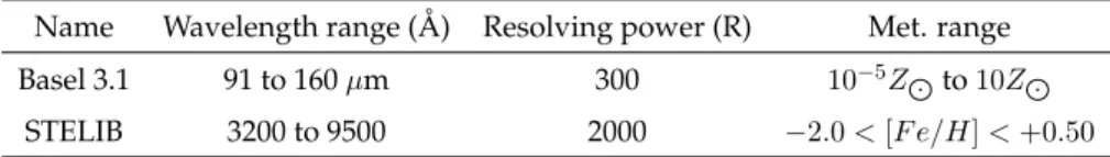
2.1 Main characteristics of the stellar spectra libraries adopted to compute BC03 models. . . 26

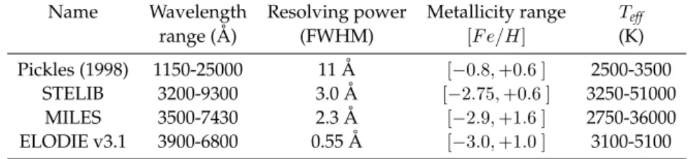
2.2 Main characteristics of the stellar spectra libraries adopted to compute MaStro models. . . 27

2.3 Spectral regions masked in the fit.. . . 31

2.4 Median shift and dispersion from the simulation of ETGs spectra, for SNR = 20 and 100 and BC03 spectral synthesis models. . . 36

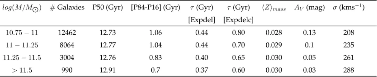
2.5 Number of galaxies, statistical, evolutionary and physical properties of the four mass bins of our sample (in the case of BC03 models). . . 50

2.6 Uncertainties on ages, metallicities, velocity dispersions and dust extinction pro-vided by the three different estimates described in the text (in the case of BC03 models). . . 58

3.1 Main ingredients of our models,Kewley et al.(2001)’s andLevesque et al.

(2010)’s ones.. . . 85

4.1 Properties of the 19 simulated spectra investigated in this Chapter. . . 121

4.2 Spectral lines masked in case 1 (emission lines only), case 2 (emission lines + ISM lines) and case 3 (emission lines + ISM lines + pure photospheric absorp-tion lines). . . 121

4.3 Median shifts and dispersions obtained for VANDELS UV simulated spectra and SNR20 50 . . . 125

(23)

(24)

The "archaeological" reconstruction

of the evolution of early-type

galaxies

The morphological dichotomy between spiral and elliptical galaxies has been known for years (i.e. since Hubble 1929). Over time, it has been observed that this bimodal-ity can be extended also to other galaxy properties, such as star formation levels and colours (e.g.Strateva et al.,2001,Kauffmann et al.,2003), resulting in a clear separation between star-forming (blue) and quiescent (red) galaxies. Understanding the origin of this dichotomy is one of the key question in the current studies of galaxy evolution. Generally, two approaches are used to investigate this issue: the backward approach, which tries to extrapolate galaxy evolution starting from the evolutionary properties of galaxies at z = 0, and the lookback studies, which infer galaxy evolution by studying the statistical properties of galaxy samples at different redshifts.

In the currently accepted ⇤CDM cosmological model, which predicts a bottom-up or hi-erarchical formation of cosmic structures, local and massive early-type galaxies (ETGs) represent the endpoints of the evolutionary process, and are therefore fundamental probes to track the galaxy cosmic history backward in cosmic time.

Morevoer, the advent of spectroscopic surveys at intermediate-high redshift (e.g. zCOS-MOS and VIPERS at z > 0.7, VVDS, VUDS, GMASS, K20, GOODS and VANDELS at z > 1 2), has allowed in the last years the statistical studies of galaxy samples at dif-ferent redshifts and thus a more accurate analysis of their evolution across cosmic time. In this chapter we discuss galaxy evolution in reverse, going from local, passive galaxies to their progenitors at high redshift. We briefly recall the properties and the relations characterizing galaxies through all the evolutionary phases, including the quenching of the star formation.

1.1 Properties of ETGs in the local and high-redshift Universe

ETGs constitute a homogeneus class of galaxies with a spheroidal (E/S0) morphology, old stellar populations, red colours, no (or negligible) star formation and high velocity dispersion (i.e. high masses). These properties are generally used to identify ETGs, and usually correlate between each other. However, it is worth noting that some past studies (e.g.Renzini,2006,Moresco et al.,2013) have argued that these classifications do not fully overlap, and thus that morphology-, photometry- or spectrum-based selection

(25)

1.1. PROPERTIES OF ETGS IN THE LOCAL AND HIGH-REDSHIFT UNIVERSE

criteria can lead to select slightly different ETG samples.

The following sections briefly recall some of the most important ETG properties and scaling relations, both in the local and high-redshift Universe.

1.1.1 Spectral properties

Due to the dominance of old stellar populations and the absence of significant ongoing star formation, ETG spectra are basically red, absorption-line spectra, as it is possible to note from Fig. 1.1. The integrated light of ETGs is dominated by old, low-mass stars (G- and K-type giants) which are still lying on the main sequence, or by stars experienc-ing advanced evolutionary stages (Red Giant Branch, Asymptotic Giant Branch), which contribute the most to the flux at long wavelengths due to their lower superficial tem-perature. Apart from the red continuum shape, ETG spectra are also characterized by several absorption features, whose strength is often related to galaxy age, metallicity (Z) and abundance ratios.Trager et al.(1998) e diWorthey & Ottaviani(1997) introduced an ensamble of 25 optical spectral features (i.e. Lick/IDS system), known as Lick indices, as powerful tools to infer galaxy properties. The general approach consists in creating synthetic indices by means of polynomial functions and evolutionary synthesis codes, and comparing them with the observed ones. Although this method is very power-ful and independent of resolving power or flux calibration limitations, it is hampered by the fact that age and metallicity may have similar effects on spectral lines and spec-tral continuum (age-metallicity degeneracy, Worthey 1994). Breaking the age-metallicity degeneracy has thus become one of the primary goals in spectroscopic studies aimed at constrain galaxy stellar population properties, and led to the search for independent in-dices separately related to age and metallicity.

In this regard, both low- (H ) and high- (e.g. H and H ) order Balmer absorption lines were proposed in the past as pure age indicators (Worthey & Ottaviani,1997,Vazdekis & Arimoto,1999), but several studies have demonstrated that they are not fully inde-pendent of metallicity or ↵-element abundance (Thomas et al.,2004,Korn et al.,2005). Moreover, moderate to high signal-to-noise ratios are required to measure them, lim-iting their use only to nearby/luminous sources. Concerning H , some authors have also shown that it can be contaminated by nebular emission (Gonzalez,1993,Concas et al.,2017). Concerning metal abundances, many of the indices proposed byWorthey

(1994) as indicators of the global metallicity (e.g. CN2, Ca4455, C24668, Fe5015, Fe5270,

Fe5335, Fe5406, Fe5709, Fe5782, NaD, TiO2) have been demonstrated to depend on the

↵-element abundance (Worthey,1994,Davies et al.,1993a,Carollo & Danziger,1994), in-troducing further uncertainties in the Lick indices method. An important step forward to disentangle between age and metallicity effects and to unambiguously determine ages, total metallicities and element abundances has consisted in creating synthetic Lick indices accounting for the effects of the ↵ elements. In particular,Tripicco & Bell(1995) determined the sensitivity of Lick absorption-line indices to individual element abun-dance variations.Trager et al.(2000) then developed a method to include these results in the analysis of stellar populations, allowing the creation of stellar population models of Lick indices with variable element abundance ratios (Thomas et al.,2003,Thomas et al.,

2005, Thomas et al.,2010). However, many uncertainties are still related to the Lick-indices approach. For instance, it is still unclear how to break the degeneracy between young stars and hot horizontal branch stars, whose presence can similarly influence the index strength. Ratios involving different indices (e.g. H F/H ), should help to

disen-tangle between the two populations (e.g. Schiavon et al.,2004), but these analyses are hampered by the ↵ elements dependence, which have to be taken into account.

(26)

The evolution of the Lick indices as a function of redshift confirm that ETGs have a high formation redshift and thus evolve passively from z ⇠ 2 3. For instance,Bender et al.

(1996) andZiegler & Bender(1997) analyzed the evolution of the Mg2index as a

func-tion of the galaxy velocity dispersion up to z = 0.375. They found a weakening of the index with cosmic time and inferred that the age of galaxies at this redshift should be about 2/3 of the age of their local counterparts, implying a zF & 3. Similar results

have been obtained by studying the evolution of the H and H spectral features (e.g.

Kelson et al.,2001). Moreover, the evolution of spectral features in galaxy spectra and the rapid decrease of the number density of massive galaxies with strong H absorption since z ⇠ 1 (Le Borgne et al.,2006,Vergani et al., 2008) gives hints on the formation scenario of ETGs, suggesting a top-down formation (see Sect.1.4).

Figure 1.1: Optical stacked spectrum of ⇠ 2800 SDSS ETGs with M ⇠ 1010.86_MJ_{and median z ⇠}

0.11. Vertical lines mark some absorption features. Black lines are metallic absorptions (from left to right: M gI, NaD); green lines are Balmer absorptions (from left to right: H , H↵); the grey shaded band mark the location of the G Band; blue shaded bands mark the location of the D4000 continuum discontinuity (also known as the D4000 break).

1.1.2 Scaling relations

Due to their homogeneity, early-type galaxies obey to well-defined scaling relations be-tween their physical and evolutionary properties, which can be used to better under-stand their galaxy structure and evolution. The following sections give a brief summary of the most important among these scaling relations.

The color-magnitude relation

The color-magnitude relation (CMR) links the (U V ) rest-frame color index to the abso-lute magnitude of elliptical galaxies, and was first discovered by Bower, Lucey & Ellis in 1992 in Virgo and Coma cluster galaxies. Very important information are enclosed in the scatter and slope of this relation, which is illustrated in Fig.1.2. In particular, assuming that ETGs are passively evolving, the scatter in the CMR allows to constrain their for-mation redshift (zf). From the observed color scatter,Bower et al.(1992) concluded that

cluster ellipticals are made of very old stars, with the bulk of star formation completed at zf& 2. This has been also confirmed by high redshift studies of the CMR. In

particu-lar,Ellis et al.(1997) andStanford et al.(1998) found that cluster ellipticals are passively evolving and have a zf & 3; analyzing field, group and cluster galaxies,Tanaka et al.

(27)

1.1. PROPERTIES OF ETGS IN THE LOCAL AND HIGH-REDSHIFT UNIVERSE

Figure 1.2: The (U V )– MV color-magnitude relation for galaxies that are spectroscopic members of the Coma cluster (from Bower et al. 1999).

faint-end is possibly still in the process of build-up. They also argued that the built-up of the field CMR appear to be delayed compared to the cluster one. It is worth remind-ing that useful evolutionary information is also enclosed in the slope of the CMR, which gives clues about the amount of merging galaxies underwent to during their evolution. Indeed, merging events can modify galaxy luminosities and velocity dispersions (dry merging) or also produce a shift in their colors (wet merging).

The fundamental plane

The fundamental plane (FP) is a relation between the structural/dynamical status of el-liptical galaxies and their stellar content (Dressler et al.,1987,Djorgovski & Davis,1987); in particular, it links ETGs effective radius Re, velocity dispersion and surface

bright-ness Ie= L/2⇡Re2so that, when ETGs are shown in the 3D space (Re, , Ie), they are not

randomly distributed, but cluster close to a plane, as illustrated in Fig.1.3. The mere ex-istence of the FP implies that elliptical galaxies are virialized systems, have homologous structures and are made of stellar populations which satisfy precise constraints in age and metallicity. However, the observed FP is ’tilted’ with respect to the theoretical rela-tion, which implies that trends in the mass-to-light ratio M/L, and hence variations in both structural and stellar properties (metallicity, initial mass function and age) must be present in the ETG population (e.g.Bender et al.,1992,Busarello et al.,1997). However, even if the nature of the small scatter at z ⇠ 0 is not clear yet, it implies that ETGs have a small age dispersion and a high formation redshift. Depending on the IMF slope and the formation redshift zf, the redshift evolution of the FP provides complementary

in-formations on the ETGs cosmic evolution. In particular, high-z FP studies in clusters led to the conclusion that it shifts nearly parallel to itself, ant thus that no trends in age or IMF with galaxy mass exists (which would produce a rotation of the FP relation); high-z FP observations in the field (Treu et al.,2005) showed, instead, that a rotation with in-creasing redshift is present and that it could be explained through a systematic trend in the M/L ratio. This trend is consistent with massive objects having a higher zfthan less

(28)

massive ones. However, the observed shift of the FP at high z is again consistent with passive evolution of more massive systems that formed at high redshift.

Figure 1.3: The infrared fundamental plane of elliptical galaxies (fromMagoulas et al.,2012).

1.1.3 Relations between evolutionary and dynamical properties of early-type

galaxies

The relations between the evolutionary and dynamical properties of early-type galax-ies in the local Universe have been proved to be particularly useful to reconstruct the galaxy evolutionary path over cosmic time. Moreover, in the past decades, these stud-ies have improved thanks to the developement of full-spectrum fitting techniques and the creation of synthetic Lick indices accounting for the presence of ↵ elements, which makes stellar population properties estimates more and more reliable (see Sect. 1.1.1). In the following, we briefly summarize three of the most important relations linking the galaxy velocity dispersion (i.e. mass) with the ↵ elements abundance ([↵/Fe]), global metallicity ([Z/H]) and age. In particular, we follow the detailed paper byThomas et al.

(2010), who derived these relations analyzing a sample of SDSS ETGs at 0.05  z  0.06.

[↵/Fe] – relation. The [↵/Fe] – relation encloses fundamental information on when and how fast ETGs formed their stars, since the [↵/Fe] ratio can be considered an in-dicator of the timescales of the star formation. ↵ elements are indeed the main prod-uct of Type II Supernovae explosions (SN II), while Fe peak elements are produced by the delayed explosion of Type Ia Supernovae. This implies that longer formation timescales correspond to lower [↵/Fe], since in this case Type Ia Supernovae have had time to dilute the ↵-elements released into the interstellar medium (ISM) by SN II explo-sions. Observations suggest that ↵ elements are more abundant in more massive ETGs (e.g. Worthey et al.,1992,Greggio,1997,Jørgensen,1999,Kuntschner,2000,Terlevich & Forbes,2002), and several studies employing synthetic Lick indices accounting for

(29)

1.2. MASS-SIZE RELATION OF ETGS

↵elements (Proctor & Sansom,2002,Thomas et al.,2002,Mehlert et al.,2003,Thomas et al.,2010) have confirmed this trend in the past decades.

[Z/H]– relation. The [Z/H] – relation links the galaxy velocity dispersion with its global metallicity. It was observed by many authors in the past decades (e.g. Greggio,

1997,Thomas et al.,2005,Thomas et al.,2010), and indicates that more massive galaxies are more metallic than less massive ones. The existence of this relation is commonly related to the galactic wind models (e.g. Arimoto & Yoshii,1987), according to which more massive galaxies, due to their deeper potential wells, are unable to produce galac-tic winds, thus retaining more metals and enriching their ISM more than less massive galaxies.

age- relation. The existence of a relation between galaxy age and velocity dispersion is still unclear and debated. However, even if early studies did not find any significant correlation between these two quantities (Trager et al.,2000, Kuntschner et al.,2001,

Terlevich & Forbes,2002), some recent works have suggested that a weak trend exists, although with a very large scatter (Proctor & Sansom,2002;Proctor et al.,2004,Thomas et al.,2005,Thomas et al.,2010). and that it goes in the direction that more massive galaxies are older than less massive ones.

These three relations, which seem also to be independent of the galaxy environment (e.g. Thomas et al.,2010), suggest that more massive galaxies are older and form stars on shorter timescales than less massive ones, paving the way for the development of the so-called downsizing scenario, described in Sect.1.4.

1.2 Mass-size relation of ETGs

The link between galaxy size and stellar mass has been studied over the past years both at low and high redshift. In the local Universe, the mass-size relation for ETGs has been observed by different authors (e.g. Bernardi et al.,2003), and defined by Shen et al.(2003) using a sample of SDSS galaxies. These authors found that the sizes of local ETGs follow a steep relation, with the median size R scaling as R / M0.55_{. Moreover,}

they argued that the observed relation is consistent with the hypothesis that early-type galaxies are the product of several merging events experienced across cosmic time, in agreeement with the ⇤CDM scenario (see Sect.1.3).

With the advent of deep surveys, this kind of investigations have been pushed towards higher and higher redshifts, and have suggested that ETGs in the past were more com-pact than their local counterparts. In particular, their effective radii Ref fat z ⇠ 2 3 can

be by up to a factor ⇠ 2 3 smaller (i.e. their density is ⇠ 30 times higher) than those in the local Universe (Trujillo et al.,2006,Toft et al.,2007,van der Wel et al.,2008,Cimatti et al.,2012) and their size evolution can be parametrized by Ref f / (1 + z) 1.48(e.g.van

der Wel et al.,2014).

It has also become clear over time that high-z ETGs are characterized by old stellar populations (e.g. Cimatti et al.,2008,van Dokkum et al.,2008) and higher velocity dis-persions than local ETGs (Cenarro & Trujillo,2009, van de Sande et al.,2011). These findings imply that most of these objects must increase their sizes and decrease their